SIMPler realisation of Scalar Dark Matter

Shivam Verma

Abstract

With growing agony of not finding a dark matter (DM) particle in direct search experiments so far (for example in XENON1T), frameworks where the freeze-out of DM is driven by number changing processes within the dark sector itself and do not contribute to direct search, like Strongly Interacting Massive Particle (SIMP) are gaining more attention. In this analysis, we ideate a simple scalar DM framework stabilised by $\mathcal{Z}_{3}$ symmetry to serve with a SIMP-like DM ( $\chi$ ) with additional light scalar mediation ( $\phi$ ) to enhance DM self interaction. We identify that a large parameter space for such DM is available from correct relic density and self interaction constraints coming from Bullet or Abell cluster data. We derive an approximate analytic solution for freeze-out of the SIMP like DM in Boltzmann equation describing $3_{\rm DM}\to 2_{\rm DM}$ number changing process within the dark sector. We also provide a comparative analysis of the SIMP like solution with the Weakly Interacting Massive Particle (WIMP) realisation of the same model framework here.

1 Introduction

Numerous experimental observations at wide range of length scales [1, 2, 3], have indicated that about 80 $\%$ of total matter density is dominated by dark matter (DM) [4, 5], although we know very little about it. The absence of a particle of its kind within the Standard Model (SM), also provides a very strong motivation for the existence of physics beyond the Standard Model. Efforts are therefore being made to characterise the nature of DM and discover them in experiments. We know of it’s existence through gravitational interaction, but as it doesn’t interact with the electromagnetic radiations, its quite hard to detect DM. Two popular ways to detect DM have so far been looked at; through Direct search, for example, XENON1T [6, 7], and Collider search, for example, Large Hadron Collider (LHC) [8]. One can also see an evidence of DM in excess of antiparticles, photon etc., however that serves as indirect search [9] of DM. After searching for more than a decade and not being able to find a DM so far, one has to evidently constrain DM properties, particularly on its coupling to the visible sector.

Amongst theoretical efforts to construct a viable DM candidate, Weakly Interacting Massive Particle (WIMPs) [10] in extensions of SM turns out to be simplest and hence most popular. In such a case, the DM is assumed to freeze-out from the equilibrium via $2_{\rm DM}\to 2_{\rm SM}$ annihilations to SM and easily satisfies the relic density $\Omega h^{2}\simeq 0.12$ (as indicated by PLANCK data [11]), if the DM-SM interaction is of the order of weak interaction strength. For WIMP like solutions, the same DM-SM interaction also provides direct search scattering and collider production. Therefore it is difficult to explain the non-observation of the DM in these experiments while addressing correct relic density. Alternate possibilities within the WIMP paradigm is therefore to decouple the number changing processes for freeze-out from direct search graphs through co-annihilation, semi-annihilation or DM-DM conversion (see for example, in [12, 13]).

Strongly Interacting Massive Particle (SIMP) predicts an interesting alternative to produce the freeze out through number changing process within the dark sector itself through for example, $3_{\rm DM}\to 2_{\rm DM}$ or $4_{\rm DM}\to 2_{\rm DM}$ processes. Evidently, for these processes to contribute significantly and govern the freeze-out, one requires very small $2_{\rm DM}\to 2_{\rm SM}$ annihilation, i.e. very small DM-SM interaction. Therefore SIMP models have a natural explanation for non-observation of DM in direct and collider searches. DM in such a framework typically has sub-GeV mass and a large self-scattering cross section, unlike the WIMP case [14]. Then, although such a large self-scattering cross section is constrained by Bullet cluster [15] and spherical halo shapes, it can lead to distinct signatures in galaxies and galaxy clusters, such as the offset of the dark matter sub halo from the galaxy centre, as hinted in Abell 3827 [16]. Recently in [14], it was shown that if we consider a paradigm where DM particles have a strong number changing self interaction, then the required thermal relic density can be obtained along with addressing the problems like core vs cusp [17] and too big to fail [18] that poses a conundrum to face.

The aim of the paper is to ideate a simple dark sector that inherits the above SIMP-like credentials. The models studied with a scalar DM so far had an additional $U(1)$ gauge symmetry to aid self interaction through additional vector boson mediation and the remnant symmetry (after symmetry breaking) stabilizes the DM [19, 20, 21, 22, 23, 24, 25]. Some other attempts to model a SIMP like DM can be seen in [26, 27, 28, 29, 30, 31, 32, 33, 34, 35, 36, 37]. We propose a dark sector consisting of one complex scalar singlet field $\chi$ and a real scalar singlet $\phi$ , where $\chi$ transforms under an unbroken $\mathcal{Z}_{3}$ symmetry and serves as DM. The scalar field $\phi$ (even under $\mathcal{Z}_{3}$ ), acquires a vacuum expectation value (vev) during spontaneous symmetry breaking (SSB) and mixes with the SM scalar doublet to predict an additional light physical scalar apart from Higgs boson, and aid DM self interaction. We perform a detailed analysis of the relic density of the DM for freeze-out through $3_{\rm DM}\to 2_{\rm DM}$ number changing process in the dark sector, with a brief sketch of $4_{\rm DM}\to 2_{\rm DM}$ process. As emphasised before, for these processes to dictate freeze-out, the Higgs portal DM-SM coupling has to be small. In this limit, we also find out that the relic density allowed parameter space is highly constrained by the DM self scattering cross-section from Bullet and Abell cluster data. The same model can also serves as WIMP DM with non vanishing Higgs portal coupling, which leads us to compare the outcome of SIMP solution to WIMP paradigm of the model.

We also make a thorough review of the Boltzmann Equation (BEQ) describing a SIMP DM (in a model independent way) and obtain an approximate analytical solution. The approximate analytical solution turns out to match closely to the numerical solution of BEQ in a wide range of DM mass.

The paper is organised as follows: Thermal freeze out for SIMP is discussed first in Section 2; the model under consideration and its relic density outcome together with self scattering cross-section constraints are discussed in Section 3; brief sketch of WIMP like solution of the model is discussed in Section 4. We finally conclude in Section 5. The Appendix of the paper is quite elaborate: DM annihilation cross-section to both DM and SM ( $3_{\rm DM}\to 2_{\rm DM}$ , $2_{\rm DM}\to 2_{\rm SM}$ , $4_{\rm DM}\to 2_{\rm DM}$ ) and scattering cross-section of DM with DM and SM are explicitly demonstrated. Freeze-out temperature of MeV order SIMP DM in the model also demonstrate in the appendix.

2 Thermal freeze out of Dark Matter in SIMP framework

In this section, we review the thermal freeze out of DM governed by BEQ. The equation can only be solved numerically. However, for a better understanding of relic density of DM governed by the number changing process within the dark sector itself (for example, $3_{\rm DM}\to 2_{\rm DM}$ process as elaborated in this paper), we will try to identify an approximate analytical solution for the corresponding BEQ. We start with a quick recap of thermal freeze-out of DM governed by $2_{\rm DM}\to 2_{\rm SM}$ annihilation, well known to yield a WIMP like solution. This will help us to construct and solve SIMP like BEQ and eventually obtain an approximate analytical solution.

2.1 A quick recap of thermal freeze-out in WIMP scenario

The very idea of thermal freeze-out of DM is based on the assumption that the DM was in thermal and chemical equilibrium in early universe. As the universe expands with Hubble rate ( $\mathcal{H}$ ), at a particular epoch the interaction rate of the DM ( $\Gamma$ ) falls below the rate of expansion ( $\mathcal{H}$ ) [10] i.e.

\mathcal{H}\>(\textrm{Hubble expansion rate})\>>\>\Gamma\>(\textrm{particle interaction rate}),

(2.1)

and the DM freezes out from equilibrium, to yield a constant DM number density in co moving volume, known as relic density. A successful DM model must yield correct relic density as observed in Cosmic Microwave Background (CMB) data for example, given by PLANCK [11]:

\displaystyle 0.1177~\leq\Omega_{{\textrm{DM}}}h^{2}\leq~0.1221,

(2.2)

where $\Omega_{{\textrm{DM}}}=\rho_{\rm DM}/\rho_{c}$ is the cosmological DM density scaled with respect to critical density $\rho_{c}=3\mathcal{H}^{2}/(8\pi G_{N})$ , with $G_{N}$ denoting Newton’s gravitational constant [10]. The phenomena of freeze-out or thermal decoupling happens when the temperature of the thermal bath falls (roughly) below the mass of the DM particle. The number density of the DM after freeze-out depends on its interaction rate ( $\Gamma$ ), which in turn depends on DM mass and coupling(s) to the visible sector. The BEQ that governs the thermal freeze-out of DM species, is described as time evolution of the DM phase space distribution function $f(\textbf{r},\textbf{p},t)$ through [10]:

\hat{\mathcal{L}}[f]=\hat{\mathcal{C}}(f),

(2.3)

where $\hat{\mathcal{L}}[f]$ is the Liouville operator describing the change in $f$ with time, while $\hat{\mathcal{C}}(f)$ denotes the change in $f$ through collision. Left hand side of the above equation remains unchanged in a homogeneous and isotropic universe (governed by Friedman-Robertson-Walker metric) ¹¹ 1 which also dictates $f(\textbf{r},P,t)\to f(E,t)$ ., while different possibilities of DM collision term $\hat{\mathcal{C}}(f)$ can yield different possibilities of DM freeze-out and relic density, as we elaborate here. The simplest realisation for the collision term $\hat{\mathcal{C}}(f)$ is obtained when two DM particles annihilate to two SM particles following the cartoon in Fig. 1.

Refer to caption — Figure 1: A cartoon of two DM particles annihilating to two SM particles to yield a WIMP-like scenario.

This is a standard number changing process for DM to yield WIMP like solution, which dictates that DM have annihilation cross-section of weak interactions strength to justify the observed relic density. The BEQ describing $2_{\rm DM}\to 2_{\rm SM}$ process can be written in terms of DM number density $n=(g_{\rm DM}/(2\pi)^{3})\int d^{3}P~f_{\rm DM}(E,t)$ as [10]:

$\displaystyle\frac{dn}{dt}+3\mathcal{H}n$	$\displaystyle=$	$\displaystyle\int\frac{g_{\rm DM}~d^{3}P_{1}}{(2\pi)^{3}2E_{1}}~\frac{g_{\rm DM}\>d^{3}P_{2}}{(2\pi)^{3}2E_{2}}~\frac{g_{\rm SM}~d^{3}P_{3}}{(2\pi)^{3}2E_{3}}~\frac{g_{\rm SM}~d^{3}P_{4}}{(2\pi)^{3}2E_{4}}(2\pi)^{4}\delta^{4}(P_{1}+P_{2}-P_{3}-P_{4})$	(2.4)
		$\displaystyle~~~~~~~~~~~~~~~~~~~~~~~~~~~~~~\times\|\mathcal{M}_{1+2\to 3+4}\|^{2}~~(f_{\rm DM}f_{\rm DM}-f_{\rm DM}^{eq}f_{\rm DM}^{eq})$
	$\displaystyle=$	$\displaystyle{-\langle\sigma v\rangle_{2_{\rm DM}\to 2_{\rm SM}}}\Big[n^{2}-{n^{eq}}^{2}\Big]~,$

where $P_{i}$ stands for three momentum of $i^{ih}$ particle, $f_{\rm DM}^{eq}\sim{e^{-{E_{\rm DM}/T}}}$ denotes Maxwell’s distribution, $g_{\rm DM}$ denotes internal degrees of freedom of DM particles, $g_{\rm SM}$ denotes internal degrees of freedom of SM particles and $\langle\sigma v\rangle_{2_{\rm DM}\to 2_{\rm SM}}$ is the thermal average annihilation cross-section given by [10, 38, 39],

$\displaystyle\langle\sigma v\rangle_{2_{\rm DM}\to 2_{\rm SM}}$	$\displaystyle=$	$\displaystyle\frac{1}{n_{1}^{eq}~n_{2}^{eq}}\int~\frac{g_{\rm DM}\>d^{3}P_{1}}{(2\pi)^{3}2E_{1}}~\frac{g_{\rm DM}\>d^{3}P_{2}}{(2\pi)^{3}2E_{2}}~\frac{g_{\rm SM}~d^{3}P_{3}}{(2\pi)^{3}2E_{3}}~\frac{g_{\rm SM}~d^{3}P_{4}}{(2\pi)^{3}2E_{4}}(2\pi)^{4}$	(2.5)
		$\displaystyle~~~~~~~~~~~~~~~~~~~~~~~~\times\delta^{4}(P_{1}+P_{2}-P_{3}-P_{4})\|\mathcal{M}_{1+2\to 3+4}\|^{2}~f_{1}^{eq}~f_{2}^{eq}~.$
	$\displaystyle=$	$\displaystyle\int_{4m_{\rm DM}^{2}}^{\infty}ds\frac{s\sqrt{(s-4m_{\rm DM}^{2})}~K_{1}(\sqrt{s}/T)~(\sigma v)_{2_{\rm DM}\to 2_{\rm SM}}}{16~T~m_{\rm DM}^{4}~[K_{2}(m_{\rm DM}/T)]^{2}}.$

One can further parameterize this equation by substituting the number density per co-moving volume: $Y=n/s$ , where $s$ is the entropy density and $x=m_{DM}/T$ to yield [10]:

\displaystyle\frac{dY}{dx}=-0.264~\frac{g_{*s}}{\sqrt{g_{*}}}~M_{pl}~\frac{m_{\rm DM}}{x^{2}}~\langle{\sigma v}\rangle_{2_{\rm DM}\to 2_{\rm SM}}~\Big(Y^{2}-Y_{eq}^{2}\Big)~.

(2.6)

In above equation,

	$\displaystyle g_{*s}$	$\displaystyle=$	$\displaystyle\sum_{i=bosons}g_{i}\Big(\frac{T_{i}}{T}\Big)^{3}+\frac{7}{8}\sum_{i=fermions}g_{i}\Big(\frac{T_{i}}{T}\Big)^{3}~,$
	$\displaystyle g_{*}$	$\displaystyle=$	$\displaystyle\sum_{i=bosons}g_{i}\Big(\frac{T_{i}}{T}\Big)^{4}+\frac{7}{8}\sum_{i=fermions}g_{i}\Big(\frac{T_{i}}{T}\Big)^{4}~,$		(2.7)

denote effective degrees of freedom associated with entropy and energy density respectively. $g_{i}$ is the degrees of freedom for the $i^{th}$ species. Since, for most of the history of the universe, all particles species shared a common temperature, it can be approximated as $g_{*s}\simeq g_{*}$ [10]. Thus, we can write 2.6 as:

\displaystyle\frac{dY}{dx}=-0.264~\sqrt{g_{*}}~M_{pl}~\frac{m_{\rm DM}}{x^{2}}~\langle{\sigma v}\rangle_{2_{\rm DM}\to 2_{\rm SM}}~\Big(Y^{2}-Y_{eq}^{2}\Big)~.

(2.8)

Using Maxwell-Boltzmann statistics for both fermions and Bosons in non-relativistic regime, the equilibrium number density per co-moving volume turns out [10]:

\displaystyle Y_{eq}(x)=0.145~\frac{g_{\rm DM}}{g_{*s}}x^{3/2}e^{-x}~.

(2.9)

For $m_{\rm DM}\sim\mathcal{O}$ (GeV), $g_{*s}\simeq g_{*}=106.75$ . With all these inputs, one can now solve the BEQ 2.8 numerically to obtain freeze out and present yield $Y(x\to\infty)$ . Using $n=s~Y(x\to\infty)$ , one can find relic density of DM as [10]:

\displaystyle\Omega h^{2}=2.752\times 10^{8}~\Big(\frac{m_{\rm DM}}{\textrm{GeV}}\Big)~Y(x\to\infty)~.

(2.10)

One can also estimate $Y(x\to\infty)$ approximately without solving BEQ numerically (Eqn.2.8) and relic density of DM can be expressed in terms of annihilation cross-section $\langle{\sigma v}\rangle_{2_{\rm DM}\to 2_{\rm SM}}$ (see for example, [10]):

\displaystyle\Omega h^{2}\approx\frac{854.45\times 10^{-13}}{\sqrt{g_{*}}}~x_{f}~\Big(\frac{{\textrm{GeV}}^{-2}}{\langle{\sigma v}\rangle_{2_{\rm DM}\to 2_{\rm SM}}}\Big)~,

(2.11)

where $x_{f}$ correspond to freeze-out temperature of DM that is given by [10]:

	$\displaystyle x_{f}$	$\displaystyle\approx$	$\displaystyle\ln\Big[0.038~\frac{g_{\rm DM}}{\sqrt{g_{*}}}~M_{Pl}~m_{\rm DM}~(c+2)c~\langle{\sigma v}\rangle_{2_{\rm DM}\to 2_{\rm SM}}\Big]$		(2.12)
			$\displaystyle~~~~~~~~~~~~~~-\frac{1}{2}\ln\ln\Big[0.038~\frac{g_{\rm DM}}{\sqrt{g_{*}}}~M_{Pl}~m_{\rm DM}~(c+2)c~\langle{\sigma v}\rangle_{2_{\rm DM}\to 2_{\rm SM}}\Big].$		(2.12)

In the above equation, at $x=x_{f}$ , $\Delta(x_{f})=cY_{eq}(x_{f})$ where $c$ is an unknown constant and $\Delta=Y-Y_{eq}$ . An example of DM freeze-out in WIMP-like scenario is shown in the right hand side (RHS) of Fig. 3 for a DM mass of 100 GeV with different values of annihilation cross-section $\langle{\sigma v}\rangle_{2_{\rm DM}\to 2_{\rm SM}}$ in $Y-x$ plane. The correct relic density $\Omega_{\rm DM}h^{2}\sim 0.12$ line is also shown, which corresponds to $\langle{\sigma v}\rangle_{2_{\rm DM}\to 2_{\rm SM}}\sim 1.5\times 10^{-9}~\rm{GeV}^{-2}$ , typical cross-section of weak interaction strength. We will now follow the same procedure to find out the freeze-out in SIMP mechanism.

2.2 SIMP scenario

SIMP mechanism can be achieved when $2_{\rm DM}\to 2_{\rm SM}$ annihilation to SM is suppressed and change in DM number density is mainly dictated within dark sector for example, by $3_{\rm DM}\rightarrow 2_{\rm DM}$ process. Given the fact that the DM still has to be in equilibrium with visible sector particles (SM particles) in thermal bath in the early universe for thermal freeze-out to provide correct relic²² 2 One can also achieve correct DM relic density, when the DM is out of equilibrium and is produced via decay or annihilation of particles in equilibrium catering to the possibility of freeze-in, see for example [40], and since DM-SM interaction is responsible for maintaining the equilibrium, it can not be completely neglected. The scattering of DM with the SM via the same interaction can still be sizeable enough even if the annihilation cross section $2_{\rm DM}\to 2_{\rm SM}$ is low due to the large SM number density compared to equilibrium DM number density (A numerical estimate is presented later in Sec. 3.5). This helps DM to keep up with equilibrium while not heating up the dark sector until the DM freezes out, following the inequality condition [14]:

\Gamma_{{\rm DM}+{\rm SM}\to{\rm DM}+{\rm SM}~\textrm{scattering}}\gtrsim~\Gamma_{3_{\rm DM}\to 2_{\rm DM}~\textrm{annihilation}}~\gg~\Gamma_{2_{\rm DM}\to 2_{\rm SM}~\textrm{annihilation}}~.

(2.13)

In above equation, $\Gamma_{{\rm DM}+{\rm SM}\to{\rm DM}+{\rm SM}}=n^{eq}~\langle\sigma v\rangle$ , $\Gamma_{2_{\rm DM}\to 2_{\rm SM}}=n\times{\langle\sigma v\rangle}_{2_{\rm DM}\to 2_{\rm SM}}$ and $\Gamma_{3_{\rm DM}\to 2_{\rm DM}}$ $=n^{2}~{\langle\sigma v^{2}\rangle}_{3_{\rm DM}\to 2_{\rm DM}}$ define the rate of the corresponding interactions, where $n$ denotes DM number density following our earlier convention. We will put up an explicit demonstration of the inequality Eq. 2.13 in context of the model described here later. The scattering does not contribute to the relic density of the DM caveat to a kinetic decoupling (see for example, the discussion on ELDER DM as in [41]); therefore the number changing processes that govern the freeze-out for SIMP can be described by the cartoon diagram of Fig. 2, where the sizes of the diagrams ( $3_{\rm DM}\to 2_{\rm DM}$ versus $2_{\rm DM}\to 2_{\rm SM}$ annihilation) roughly indicate the dominant and sub-dominant contributions.

Thermally averaged cross section for $n\rightarrow 2$ annihilation processes, where n is the initial number of DM particle and 2 correspond to the number of particles in the final state can be expressed in terms of the characteristic mass scale $M$ as [30]:

[<\sigma_{n\rightarrow 2}v^{n-1}>]=[M^{-3n+4}].

(2.14)

Eq. 2.14 can simply be derived from equating the Hubble constant ( $\mathcal{H}$ ) to the rate of interaction ( $\Gamma$ ) for $n\rightarrow 2$ annihilation process. According to Eq. 2.14, a $2_{\rm DM}\to 2_{\rm SM}$ process is: $[\langle\sigma v\rangle]=[M]^{-2}$ , with unit $\rm{GeV}^{-2}$ (assuming the mass of the DM $\sim$ GeV and ’v’ to be dimensionless in natural units). Similarly for a $3_{\rm DM}\to 2_{\rm DM}$ process, $[\langle\sigma v^{2}\rangle]=[M]^{-5}$ , so it has unit $\rm{GeV}^{-5}$ and for $4_{\rm DM}\to 2_{\rm DM}$ process, $[\langle\sigma v^{3}\rangle]=[M]^{-8}$ , with unit $\rm{GeV}^{-8}$ . Next we discuss BEQ for $3_{\rm DM}\to 2_{\rm DM}$ process and its possible analytical solutions for freeze-out.

2.2.1 Boltzmann Equation and numerical solution to freeze-out

The BEQ that dictates the freeze-out through $3_{\rm DM}\to 2_{\rm DM}$ number changing process in dark sector (see Fig. 2a only), in terms of DM number density, n [10, 32] is given by ³³ 3 As argued before, DM-SM interaction can not be neglected for the DM to be in thermal bath, however contribution of $2_{\rm DM}\to 2_{\rm SM}$ for the DM freeze-out can be neglected in SIMP paradigm.:

$\displaystyle\frac{dn}{dt}+3\mathcal{H}n$	$\displaystyle=$	$\displaystyle\int\frac{g_{\rm DM}~d^{3}P_{1}}{(2\pi)^{3}2E_{1}}~\frac{g_{DM}\>d^{3}P_{2}}{(2\pi)^{3}2E_{2}}~\frac{g_{\rm DM}~d^{3}P_{3}}{(2\pi)^{3}2E_{3}}~\frac{g_{\rm DM}~d^{3}P_{4}}{(2\pi)^{3}2E_{4}}~\frac{g_{DM}~d^{3}P_{5}}{(2\pi)^{3}2E_{5}}~(2\pi)^{4}$	(2.15)
		$\displaystyle~\delta^{4}(P_{1}+P_{2}+P_{3}-P_{4}-P_{5})\times\overline{\|\mathcal{M}_{1+2+3\to 4+5}\|^{2}}\times(f_{\rm DM}~f_{\rm DM}~f_{\rm DM}-f_{\rm DM}^{eq}~f_{\rm DM}^{eq})$
	$\displaystyle=$	$\displaystyle-\langle\sigma v^{2}\rangle_{3_{\rm DM}\to 2_{\rm DM}}\Big(n^{3}-n^{2}{n^{eq}}\Big),$

where again $g_{\rm DM}$ denotes the internal degrees of freedom in the DM sector. The thermal average of annihilation cross section $\langle\sigma v^{2}\rangle_{3_{\rm DM}\to 2_{\rm DM}}$ in this case is given by [32]:

	$\displaystyle\langle\sigma v^{2}\rangle_{3_{\rm DM}\to 2_{\rm DM}}$	$\displaystyle=$	$\displaystyle\frac{1}{n_{1}^{eq}~n_{2}^{eq}~n_{3}^{eq}}\int\frac{g_{\rm DM}~d^{3}P_{1}}{(2\pi)^{3}2E_{1}}~\frac{g_{\rm DM}\>d^{3}P_{2}}{(2\pi)^{3}2E_{2}}~\frac{g_{\rm DM}~d^{3}P_{3}}{(2\pi)^{3}2E_{3}}~\frac{g_{\rm DM}~d^{3}P_{4}}{(2\pi)^{3}2E_{4}}~\frac{g_{\rm DM}~d^{3}P_{5}}{(2\pi)^{3}2E_{5}}$		(2.16)
			$\displaystyle~~~~~(2\pi)^{4}\delta^{4}(P_{1}+P_{2}+P_{3}-P_{4}-P_{5})\times\overline{\|\mathcal{M}_{1+2+3\to 4+5}\|^{2}}f_{1}^{eq}f_{2}^{eq}f_{3}^{eq}$		(2.16)

In terms of co-moving number density, i.e. $Y=n/s$ and $x=m_{\rm DM}/T$ , the BEQ turns out to be [10]:

\displaystyle\frac{dY}{dx}=-0.116~\frac{g_{*s}^{2}}{\sqrt{g_{*}}}~M_{Pl}\frac{{m_{\rm DM}}^{4}}{x^{5}}~\langle{\sigma v^{2}}\rangle_{3_{\rm DM}\to 2_{\rm DM}}~\Big(Y^{3}-Y^{2}~Y_{eq}\Big).

(2.17)

Since the temperature scale considered here allows us to take $g_{*s}\simeq g_{*}$ , we can rewrite the above BEQ as,

\displaystyle\frac{dY}{dx}=-0.116~g_{*}^{3/2}~M_{Pl}\frac{{m_{\rm DM}}^{4}}{x^{5}}~\langle{\sigma v^{2}}\rangle_{3_{\rm DM}\to 2_{\rm DM}}~\Big(Y^{3}-Y^{2}~Y_{eq}\Big).

(2.18)

The equilibrium yield is $Y_{eq}(x)=0.145~(g_{\rm DM}/g_{*s})x^{3/2}e^{-x}$ , with $g_{*s}\simeq g_{*}=10.75$ for MeV order DM. Again, one can solve the BEQ (Eq. 2.17) numerically to find the yield after freeze out: $Y(x\to\infty)$ . One such numerical solution is demonstrated in the left panel of Fig. 3. For illustration, we have chosen mass of the DM to be 100 MeV and different magnitudes of annihilation cross-section to lie within: $\langle{\sigma v^{2}}\rangle_{3_{\rm DM}\to 2_{\rm DM}}\sim\{10^{4}-10^{9}\}\rm{GeV}^{-5}$ . The one corresponding to correct relic density (horizontal black dashed line in left panel of Fig. 3) is $\langle{\sigma v^{2}}\rangle_{3_{\rm DM}\to 2_{\rm DM}}\sim 2.5\times 10^{6}~\rm{GeV}^{-5}$ , that lies in the strong interaction range. This can now be contrasted to WIMP case ( $2_{\rm DM}\to 2_{\rm SM}$ ) on the right panel graph, where correct relic density is obtained for 100 GeV DM with $\langle{\sigma v}\rangle_{2_{\rm DM}\to 2_{\rm SM}}\sim 1.5\times 10^{-9}~\rm{GeV}^{-2}$ . As stated earlier, relic density of DM in terms of yield after freeze out reads as [10, 39]:

	$\displaystyle\Omega h^{2}$	$\displaystyle=$	$\displaystyle 2.752\times 10^{8}~\Big(\frac{m_{\rm DM}}{\textrm{GeV}}\Big)~Y(x\to\infty)~,$		(2.19)
		$\displaystyle=$	$\displaystyle 2.752\times 10^{5}~\Big(\frac{m_{\rm DM}}{\textrm{MeV}}\Big)~Y(x\to\infty)~,$		(2.19)

where the numerical pre factor depends on the choice of DM mass to be in MeV or in GeV order.

2.2.2 Approximate analytical solution to Boltzmann Equation

The main idea of this section is to find an approximate analytical solution for BEQ governed by $3_{\rm DM}\to 2_{\rm DM}$ process as in Eq. 2.17. Such an exercise is already standardised for $2_{\rm DM}\to 2_{\rm SM}$ case and we will follow a similar path. We first rewrite the BEQ (Eq. 2.17) in terms of $\Delta=Y-Y_{eq}$ , that marks the difference of DM yield from the corresponding equilibrium yield. When $\Delta$ is small, the DM follows equilibrium distribution, when $\Delta$ turns large, the DM freezes out. The BEQ in terms of $\Delta$ reads as [10]:

\displaystyle\frac{d\Delta}{dx}+\frac{dY_{eq}}{dx}

\displaystyle=

\displaystyle-\frac{A}{x^{5}}\Delta\Big(Y_{eq}^{2}+2\Delta Y_{eq}+\Delta^{2}\Big)~,

(2.20)

where we have dumped everything else into $A=0.116~{g_{*}}^{\frac{3}{2}}~M_{Pl}~{m_{\rm DM}}^{4}~\langle{\sigma v^{2}}\rangle_{3_{\rm DM}\to 2_{\rm DM}}$ . Before freeze-out, i.e. for $1<x\leq x_{f}$ ( $x_{f}$ denotes freeze out of DM), $\Delta<<Y_{eq}$ and $d\Delta/dx\to 0$ . Then BEQ simplifies to:

\displaystyle\frac{dY_{eq}}{dx}

\displaystyle=

\displaystyle-\frac{A}{x^{5}}\Delta\Big((Y_{eq})^{2}+2\Delta Y_{eq}+\Delta^{2}\Big)~.

(2.21)

Near freeze-out, i.e. for $x\sim x_{f}$ , one can assume $\Delta(x_{f})=c~Y_{eq}(x_{f})$ [10] where $c$ is an unknown constant. The BEQ in such a case turns out to be:

$\displaystyle\frac{dY_{eq}}{dx}\|_{x=x_{f}}$	$\displaystyle=$	$\displaystyle-\frac{A}{x_{f}^{5}}\Delta(x_{f})~\Big(Y_{eq}^{2}(x_{f})+2\Delta(x_{f})~Y_{eq}(x_{f})+{\Delta^{2}(x_{f})}\Big)~,$
$\displaystyle\Rightarrow\Big(1-\frac{3}{2x_{f}}\Big)$	$\displaystyle=$	$\displaystyle\frac{A}{x_{f}^{5}}c(c+1)^{2}Y_{eq}^{2}(x_{f})\hskip 71.13188pt~~~~~~~~~~~~\bigg[{\rm using}\;\Delta(x_{f})=c~Y_{eq}(x_{f})\bigg]$
$\displaystyle\Rightarrow\Big(1-\frac{3}{2x_{f}}\Big)$	$\displaystyle=$	$\displaystyle\frac{A}{x_{f}^{5}}c(c+1)^{2}\Big(0.145~\frac{g_{\rm DM}}{g_{}}x_{f}^{3/2}e^{-x_{f}}\Big)^{2}~~\bigg[{\rm using}~Y_{eq}=0.145~\frac{g_{\rm DM}}{g_{}}x^{3/2}e^{-x}\bigg]$
$\displaystyle\Rightarrow\Big(x_{f}^{2}-\frac{3}{2}x_{f}\Big)$	$\displaystyle=$	$\displaystyle 0.0024\frac{g_{\rm DM}^{2}}{\sqrt{g}_{*}}~c(c+1)^{2}~M_{Pl}~m_{\rm DM}^{4}~\langle{\sigma v^{2}}\rangle_{3_{\rm DM}\to 2_{\rm DM}}~e^{-2x_{f}}~~~~~~~~~\>\bigg[{\rm using}~A\bigg]$
$\displaystyle\Rightarrow x_{f}^{2}$	$\displaystyle=$	$\displaystyle 0.0024\frac{g_{\rm DM}^{2}}{\sqrt{g}_{*}}~c(c+1)^{2}~M_{Pl}~m_{\rm DM}^{4}~\langle{\sigma v^{2}}\rangle_{3_{\rm DM}\to 2_{\rm DM}}~e^{-2x_{f}}$	(2.22)

One can solve for $x_{f}$ iteratively from above equation to obtain:

	$\displaystyle x_{f}$		$\displaystyle\approx\frac{1}{2}\ln\Big[0.0024\frac{g_{\rm DM}^{2}}{\sqrt{g}_{*}}~c(c+1)^{2}~M_{Pl}~m_{\rm DM}^{4}~\langle{\sigma v^{2}}\rangle_{3_{\rm DM}\to 2_{\rm DM}}\Big]$		(2.23)
			$\displaystyle~~~-2\ln\Big[\frac{1}{2}\ln\Big[0.0024\frac{g_{\rm DM}^{2}}{\sqrt{g}_{*}}~c(c+1)^{2}~M_{Pl}~m_{\rm DM}^{4}~\langle{\sigma v^{2}}\rangle_{3_{\rm DM}\to 2_{\rm DM}}\Big]\Big]$		(2.23)

Therefore, given the knowledge of DM mass and annihilation cross-section $\langle{\sigma v^{2}}\rangle_{3_{\rm DM}\to 2_{\rm DM}}$ , one can find the decoupling or freeze-out temperature $x_{f}$ . It is straightforward to show that for correct relic density (for example, with $m_{\rm DM}\sim 100$ MeV and $\langle{\sigma v^{2}}\rangle_{3_{\rm DM}\to 2_{\rm DM}}\sim 2.5\times 10^{6}~\rm{GeV}^{-5}$ as shown in the left panel of Fig. 3), $x_{f}\sim 20$ , which is similar to WIMP like scenarios. This is shown in Fig. 4 for different values of the unknown constant $c$ as a function of DM mass. We see that a large variation in $c$ produces only a small change in $x_{f}$ and indicate the stability of the solution.

To evaluate relic density of DM, one needs to find out the yield after freeze out. We therefore need to focus at $x>>x_{f}$ , where $Y_{eq}\to 0$ . The Eq. 2.20 simplifies to a great extent to take the following form:

$\displaystyle\frac{d\Delta}{dx}$	$\displaystyle=$	$\displaystyle-\frac{A}{x^{5}}\Delta^{3}~$	(2.24)
$\displaystyle\int_{\Delta(x_{f})}^{\Delta(x\to\infty)}-\frac{d\Delta}{\Delta^{3}}$	$\displaystyle=$	$\displaystyle A\int_{x_{f}}^{\infty}\frac{dx}{x^{5}}$
$\displaystyle\Rightarrow\frac{1}{\Delta(x\to\infty)^{2}}$	$\displaystyle=$	$\displaystyle\frac{A^{2}Y_{eq}^{2}}{x_{f}^{10}}+\frac{A}{2x_{f}^{4}}=\frac{A(2AY_{eq}^{2}+x_{f}^{6})}{2x_{f}^{10}}~~\bigg[\rm{from}\>Eq.\ref{deltaxf},\Delta(x_{f})=\frac{x_{f}^{5}}{A\>Y_{eq}(x_{f})}\bigg]$
$\displaystyle\Rightarrow\Delta(x\to\infty)$	$\displaystyle=$	$\displaystyle\sqrt{\frac{2}{A}}~x_{f}^{2}\hskip 85.35826pt~~~~~~~~~~~~~~~~~~~~~~~~~~~~~~~~~~~\Bigg[A\>Y_{eq}^{2}<<x_{f}^{6}\bigg]$
$\displaystyle\Rightarrow Y(x\to\infty)$	$\displaystyle=$	$\displaystyle x_{f}^{2}~~\sqrt{\frac{2}{0.12g_{*}^{\frac{3}{2}}~M_{Pl}~m_{DM}^{4}~\langle{\sigma v^{2}}\rangle}_{3_{\rm DM}\to 2_{\rm DM}}}.$	(2.25)

Now, From Eq. 2.19 and Eq. 2.25, one can write the expression of relic density as follows:

	$\displaystyle\Omega h^{2}$	$\displaystyle=$	$\displaystyle 2.752\times 10^{8}\left(\frac{m_{\rm DM}}{{\textrm{MeV}\times 10^{3}}}\right)\times\sqrt{\frac{2}{0.12g_{*}^{\frac{3}{2}}~M_{Pl}~m_{\rm DM}^{4}~\langle{\sigma v^{2}}\rangle_{3_{\rm DM}\to 2_{\rm DM}}}}~x_{f}^{2}$		(2.26)
		$\displaystyle=$	$\displaystyle\frac{0.33}{{g_{*}}^{\frac{3}{4}}}\Big(\frac{\textrm{MeV}\times 10^{3}}{m_{\rm DM}}\Big)~x_{f}^{2}~\sqrt{\Big(\frac{{\textrm{GeV}}^{-5}}{\langle{\sigma v^{2}}\rangle_{3_{\rm DM}\to 2_{\rm DM}}}\Big)}~.$		(2.26)

Now, we are in a position to check the reliability of the analytical solution for DM relic density obtained for the SIMP like case (Eq. 2.26) to that of the numerical solution obtained from the BEQ 2.17. This is shown in Fig. 5, where we plot relic density obtained from both numerical solution and approximate analytical solution together for different values of $c$ . Two different annihilation cross-sections $\langle\sigma v^{2}\rangle_{3_{\rm DM}\to 2_{\rm DM}}=\{2\times 10^{6},10^{9}\}~{\rm GeV^{-5}}$ are shown in left and right panel respectively. We see from Fig.5, that the analytical solution closely mimic the numerical solution for higher values of DM mass ( $\sim$ GeV). Actually, the cause of this discrepancy in relic density obtained between numerical and analytical solution occurs when we simplify the Eq.2.20 to Eq.2.25 to only retain terms of the order $\sim\Delta^{3}$ . If we consider second order term in $\Delta(x)$ , the equation looks like that of Abel equation of first kind [42], solution of that will mimic the numerical solution even more closely.

3 Model specific analysis of a SIMP Framework

3.1 The Model

If simplicity is the guiding principle to realise a SIMP paradigm, one should focus on scalar DM ( $\chi$ ). The DM also need to possess an additional symmetry for stability (call it a dark symmetry) distinct from that of the SM. If we require a vertex consisting of three DM fields ( $\chi^{3}$ ) for the DM to enable a $3_{\rm DM}\to 2_{\rm DM}$ interaction, the minimal choice for the symmetry under which $\chi$ transforms non trivially is $\mathcal{Z}_{3}$ . As the roots of $\mathcal{Z}_{3}$ are complex ( $1,\omega,\omega^{2}$ ), the scalar DM $\chi$ needs to be complex. In principle, this is enough to ideate $3_{\rm DM}\to 2_{\rm DM}$ interactions through $\chi$ mediation itself. However, it turns out that relic density allowed parameter space for this simplest possibility is quite restrictive and even more so when we impose the self scattering (we will have explicit demonstration later) and unitarity bound. We can enlarge the available parameter space by connecting the graph for $3_{\rm DM}\to 2_{\rm DM}$ process to the other end in presence of a mediator, which doesn’t have $\mathcal{Z}_{3}$ charge. But, this can not be realised with a SM particle (even if Higgs has a portal interaction with our DM) unless we augment the SM with another additional field. Again, the minimal choice of such mediator will be another scalar $\phi$ (real scalar for simplicity) which is singlet under SM.

Therefore, in this model, we consider a complex scalar singlet field $\chi$ which transforms under $\mathcal{Z}_{3}$ and acts as DM, while the real scalar singlet $\phi$ do not transform under $\mathcal{Z}_{3}$ . The $\mathcal{Z}_{3}$ transformation properties of the fields is mentioned in Table 1. In SIMP paradigm, the freeze out is mainly driven by $3_{\rm DM}\to 2_{\rm DM}$ number changing process, so the $2_{\rm DM}\to 2_{\rm SM}$ interaction can be killed by choosing a negligible value of the Higgs portal coupling. Now, if we provide VEV to $\phi$ , then it will mix with SM Higgs after spontaneous symmetry breaking and will mediate the number changing process in the dark sector. The mass of the additional scalar can be fairly light (being singlet) and will aid to annihilation cross-section providing cushion to the DM coupling to remain within perturbative limit.

Particle	Nature	$\mathcal{Z}_{3}$ transformation
$\chi$	Complex Scalar Singlet	$\omega$
$\phi$	Real Scalar Singlet	1
$H$	SM Higgs Doublet	$1$

Table 1:

\mathcal{Z}_{3}

charges of the additional scalar fields assumed in the model (

\chi,\phi

The relevant Lagrangian for this model can be mainly segregated into two parts :

\mathcal{L}=\mathcal{L}_{\textrm{SM}}+\mathcal{L}_{\textrm{BSM}}.

(3.1)

Here, we are interested in the part describing the dark sector:

\mathcal{L}_{\textrm{BSM}}=\frac{1}{2}(\partial^{\mu}\phi)(\partial_{\mu}\phi)+(\partial^{\mu}\chi)^{*}(\partial_{\mu}\chi)-V(H,\phi,\chi).

(3.2)

The scalar potential involving the additional scalars and SM Higgs ( $H$ ) reads as [14, 43]:

$\displaystyle V(H,\phi,\chi)$	$\displaystyle=$	$\displaystyle-\mu_{H}^{2}H^{\dagger}H+\lambda_{H}(H^{\dagger}H)^{2}-\frac{1}{2}\mu_{\phi}^{2}\phi^{2}+\frac{1}{4}\lambda_{\phi}~\phi^{4}$	(3.3)
		$\displaystyle+\frac{\mu_{3}}{3}\phi^{3}+\frac{1}{2}\lambda_{\phi h}~\phi^{2}~H^{\dagger}H+\mu_{\phi h}~\phi~(H^{\dagger}H)$
		$\displaystyle+\mu^{2}\|\chi\|^{2}+\lambda_{\chi}\|\chi\|^{4}+\frac{1}{3!}\mu_{\chi}(\chi^{3}+\chi^{*3})+\lambda_{\chi h}~\|\chi\|^{2}H^{\dagger}H$
		$\displaystyle+\frac{1}{2}\lambda_{\chi\phi}\|\chi\|^{2}\phi^{2}+\mu_{\chi\phi}~\phi~\|\chi\|^{2}+\frac{1}{3!}Y_{\chi\phi}~\phi~(\chi^{3}+\chi^{*3}).$

As has already been mentioned, $3_{\rm DM}\to 2_{\rm DM}$ interactions are mediated by the self couplings of $\chi$ , namely involving $|\chi|^{4}$ and $\chi^{3}$ terms. $\phi$ mediates additional channels through the two terms $\chi^{3}\phi$ and $|\chi|^{2}\phi^{2}$ , when $\phi$ acquires a VEV. After spontaneous symmetry breaking (SSB), $\phi$ and $H$ mixes through their VEVs ( $v_{\phi}$ and $v_{h}$ ) as follows:

	$\displaystyle\phi\to\Phi+v_{\phi},$		(3.4)
	$\displaystyle H\to\begin{pmatrix}0\\ \frac{h+v_{h}}{\sqrt{2}}\end{pmatrix}.$		(3.5)

The squared mass matrix for the interaction basis, $(h~\Phi)^{T}$ is given as,

\displaystyle M^{2}_{h\Phi}=\begin{pmatrix}2v_{h}^{2}\lambda_{h}&\>v_{h}v_{\phi}\lambda_{\phi h}+v_{h}\mu_{h\phi}\\ v_{h}v_{\phi}\lambda_{\phi h}+v_{h}\mu_{h\phi}&\quad\mu_{3}v_{\phi}+2v_{\phi}^{2}\lambda_{\phi}-\mu_{h\phi}(v_{h}^{2}/2v_{\phi}),\end{pmatrix}=\begin{pmatrix}A&B\\ B&C\end{pmatrix}.

(3.6)

The physical scalars ( $h_{1}$ and $h_{2}$ ) are obtained from $h,\Phi$ by choosing the following transformation,

\displaystyle\begin{pmatrix}h_{1}\\ h_{2}\end{pmatrix}=\begin{pmatrix}\cos\theta&-\sin\theta\\ \sin\theta&\cos\theta\end{pmatrix}\begin{pmatrix}h\\ \Phi\end{pmatrix}

(3.7)

The mass eigenvalues are therefore obtained by diagonalising the above mass matrix ( $M^{2}_{h\Phi}$ ) and are given by:

	$\displaystyle m_{h_{1}}^{2}=$	$\displaystyle A\>\cos^{2}\theta+C\>\sin^{2}\theta-B\>\sin 2\theta$		(3.8)
	$\displaystyle m_{h_{2}}^{2}=$	$\displaystyle A\>\sin^{2}\theta+C\>\cos^{2}\theta+B\>\sin 2\theta.$		(3.8)

The physical states are related to the flavour states through the mixing angle $\theta$ as:

\displaystyle\tan\>2\theta=\frac{2B}{C-A}

(3.9)

Now, we are all set to address the phenomenology of the scalar sector. Let $h_{2}$ be the SM like Higgs ( $m_{h_{2}}=125~{\rm GeV}$ and $v_{h}=246~{\rm GeV}$ ) and $h_{1}$ be the additional scalar boson. The additional scalar being a singlet predominantly, can be heavier or lighter than the SM Higgs, because it can’t be produced at colliders easily. We will be interested in the light Higgs mass region, where we will have $\sin\theta\to 1$ , for above mixing assignment. Finally, we point out that we can easily rewrite some of the coupling parameters as a function of the physical masses after SSB as follows [14, 44, 45]:

$\displaystyle\mu_{\text{$\phi$h}}$	$\displaystyle=$	$\displaystyle-\frac{2v_{\phi}}{v_{h}^{2}}\bigg(\sin^{2}\theta m_{h_{1}}^{2}+\cos^{2}\theta m_{h_{2}}^{2}+v_{\phi}\left(-2\lambda_{\phi}v_{\phi}+\mu_{3}\right)\bigg)~,$
$\displaystyle\lambda_{\text{$\phi$h}}$	$\displaystyle=$	$\displaystyle\frac{1}{v_{h}v_{\phi}}\bigg(\text{sin$\theta$}\>\text{cos$\theta$}\left(m_{h_{2}}^{2}-m_{h_{1}}^{2}\right)-v_{h}\mu_{\text{$\phi$h}}\bigg)~,$
$\displaystyle\lambda_{h}$	$\displaystyle=$	$\displaystyle\frac{1}{2v_{h}^{2}}\bigg(\sin^{2}\theta m_{h_{2}}^{2}+\cos^{2}\theta m_{h_{1}}^{2}\bigg).$	(3.10)

The freedom of choosing other parameters will help us to get a correct Higgs mass even if we vary the following parameters to address correct relic density for DM in this model:

\{m_{\chi}(=m_{\rm DM}),Y_{\chi\phi},\sin\theta,\lambda_{\chi\phi},\lambda_{\chi h},m_{h_{1}},v_{\phi},\mu_{\chi},\mu_{\chi\phi},\lambda_{\chi}\}~.

(3.11)

After SSB the DM mass turns out to be : $m_{\chi}^{2}=\mu^{2}+\frac{1}{2}~\lambda_{\chi\phi}~v_{\phi}^{2}+\mu_{\chi\phi}~v_{\phi}+\frac{1}{2}\lambda_{\chi h}~v_{h}^{2}$ . Again, due to large number of parameters dictating DM mass, we will vary DM mass ( $m_{\chi}$ ), along with ( $\mu_{\chi},v_{\phi},Y_{\chi\phi}$ ) independently to search for available parameter space of the model.

3.2 Relic density outcome

The model at hand offers both SIMP like and WIMP like solution as it has both self coupling and coupling to SM. For SIMP framework to be operative, a very tiny coupling with SM is realised by taming $\lambda_{\chi h}$ and $\lambda_{\chi\phi}$ . The Feynman diagrams that leads to $3_{\rm DM}\to 2_{\rm DM}$ number changing processes in this framework are shown in Appendix B. There are four annihilation processes that dictate relic density of the DM, they are $\chi\chi\chi\to\chi\chi^{*}$ , $\chi\chi^{*}\chi^{*}\to\chi\chi$ and their complex conjugate processes i.e. $\chi^{*}\chi^{*}\chi^{*}\to\chi^{*}\chi$ and $\chi^{*}\chi\chi\to\chi^{*}\chi^{*}$ respectively ⁴⁴ 4 One may note that in presence of $\mathcal{Z}_{3}$ symmetry, one may also have semi annihilations like $\chi\chi\to\chi^{*}h_{1}$ or $\chi\chi\chi^{*}\to\chi^{*}\chi^{*}h_{1}$ . However, their contributions will be small due to small $\lambda_{\chi h}$ and $\lambda_{\chi\phi}$ couplings assumed for SIMP realisation to work. The diagrams in each cases can be categorized into two classes, (i) mediated by self interaction of $\chi$ , (ii) mediated by the scalars $h_{1}~\&~h_{2}$ . We implemented this model using LanHEP [46]. To check the consistency with our numerical calculations, we have used CalcHEP [47], for drawing the Feynman diagrams we have used Tikz-Feynhand [48] and in order to calculate the matrix amplitude and relic density, we have used Mathematica [49]. Vertex factors used in the calculation of each matrix amplitudes are also detailed in Appendix B. Here we note that the numerical solution to the SIMP like BEQ have been used to scan the parameter space to yield relic density, instead of the approximate analytical solution advocated before.

It is straightforward to see that the matrix element squared for the complex conjugate processes are same:

|\mathcal{M}_{\chi\chi\chi\to\chi\chi^{*}}|^{2}=|\mathcal{M}_{\chi^{*}\chi^{*}\chi^{*}\to\chi^{*}\chi}|^{2},~|\mathcal{M}_{\chi\chi^{*}\chi^{*}\to\chi\chi}|^{2}=|\mathcal{M}_{\chi^{*}\chi\chi\to\chi^{*}\chi^{*}}|^{2}.

Therefore, the total $3_{\rm DM}\to 2_{\rm DM}$ annihilation cross section in this model is given by:

	$\displaystyle\langle\sigma v^{2}\rangle_{3_{\rm DM}\to 2_{\rm DM}}$	$\displaystyle=$	$\displaystyle 2[\langle\sigma_{\chi\chi\chi\to\chi\chi^{}}v^{2}\rangle+\langle\sigma_{\chi\chi^{}\chi^{*}\to\chi\chi}v^{2}\rangle]~,$		(3.12)
		$\displaystyle=$	$\displaystyle\frac{2\sqrt{5}}{192\pi m_{\chi}^{3}}\bigg(\|\mathcal{M}_{\chi\chi\chi\to\chi\chi^{}}\|^{2}+\|\mathcal{M}_{\chi\chi^{}\chi^{*}\to\chi\chi}\|^{2}\bigg),$		(3.12)

where the last line corresponds to $s$ -wave computation of the annihilation cross section, also detailed in appendix B. For SIMP realization, we choose $\lambda_{\chi\phi}$ and $\lambda_{\chi h}$ very tiny $\sim 0.001$ . Since we are also interested in exploring the light Higgs mediation to expedite the annihilation processes, we have kept the value of mixing angle $\sin\theta=0.999(\to 1)$ . Keeping above parameters as quoted, we are now left with the following free parameters:

\{m_{\chi},Y_{\chi\phi},m_{h_{1}},v_{\phi},\mu_{\chi},\mu_{\chi\phi},\lambda_{\chi}\}.

(3.13)

Now we will study the variation of relic density with DM mass, keeping most of the other parameters steady. In Fig. 6, we show such a variation with respect to different choices of $Y_{\chi\phi}\sim\{0.001\to 1\}$ in the left panel and for different choices of $v_{\phi}\sim\{30m_{\chi}\to 120m_{\chi}\}$ in the right panel (the parameters kept constant are mentioned in the figure inset). We have kept $\lambda_{\chi}=1$ for both the plots. The outcome from the left panel is understood easily, with larger $Y_{\chi\phi}$ , the $3_{\rm DM}\to 2_{\rm DM}$ annihilation gets larger and that diminishes the relic density significantly. Therefore, $Y_{\chi\phi}$ serves as one of the key parameters to find correct relic density in this model, and is used for the numerical scan performed later. Similarly, from the right panel, we see that $v_{\phi}$ turns out to be an important parameter to find the correct relic of this DM, as with larger $v_{\phi}$ , the annihilation cross-section increases and subsequently the relic density drops. The effects of $Y_{\chi\phi}$ and $v_{\phi}$ can also be validated from the expressions of annihilation cross-sections detailed in Appendix B. As stated before, we use the numerical solution obtained from the BEQ.

Next in Fig. 7, we show the relic density allowed parameter space in $m_{\chi}-Y_{\chi\phi}$ plane by varying $m_{h_{1}}$ (Top Left), $\mu_{\chi}$ (Top Right), $\mu_{\chi\phi}$ (Bottom Left) and $v_{\phi}$ (Bottom Right) with other parameters fixed as mentioned in figure inset. We again choose $\lambda_{\chi}=1$ for this plot. The available parameter space has a large DM mass range upto GeV with larger $Y_{\chi\phi}$ (going upto 0.4). We also see that variation in $\mu_{\chi}$ and $v_{\phi}$ affect relic density quite significantly (top right and bottom right respectively) allowing a wide span of relic density allowed parameter space. This is easily seen from the vertex factors in Appendix B, that the three point vertex is directly proportional to $\mu_{\chi}$ and also on $v_{\phi}$ thanks to $\phi\chi^{3}$ term, which crucially controls the annihilation cross-section through self mediation. From the top left figure in Fig. 7, we also see that a light scalar (red points depicted by choosing $m_{h_{1}}=0.05m_{\chi}$ ) show a departure from the choices of heavy scalar ( $m_{h_{1}}=m_{\chi},25m_{\chi}$ shown by cyan and dark blue points) for sufficiently small DM mass $\leq 150$ MeV. Again, note here that due to the freedom of having a large number of parameters contributing to $m_{h_{1,2}}$ , we can fix Higgs mass ( $m_{h_{2}}$ ) to 125 GeV and still vary $m_{h_{1}}$ keeping $v_{\phi}=60m_{\chi}$ as in the top left panel. Also note here, that stability of the scalar potential constrains the dimensionful cubic couplings $\mu_{\chi}$ and $\mu_{\chi\phi}$ to lie within $3m_{\chi}$ in a conservative limit as adopted for the scans.

To summarise this section, we see that a large parameter space is available from relic density constraint, particularly the DM mass can vary in a large range even upto GeV, while the relevant couplings $Y_{\chi\phi},\lambda_{\chi}$ do not require to be very large. These are all in contrary to the naive SIMP realisation of DM ideally having one self coupling and one mass parameter dictating them to be in the strong interaction range. However, we need to consider other constraints like unitarity, vacuum stability and self scattering cross section, which will constrain the relic density allowed parameter space as we discuss below.

3.3 Additional Constraints on dark matter parameter space

In this section, we discuss three important constraints on the model parameter space coming from vacuum stability, unitarity and DM self interaction cross-section limit. All the couplings are assumed positive to cope up with the vacuum stability of the scalar potential.

3.3.1 Self scattering cross section

DM self scatters through $2_{\rm DM}\to 2_{\rm DM}$ scattering process like $\chi\chi\to\chi\chi$ and $\chi\chi^{*}\to\chi\chi^{*}$ and their complex conjugate processes. Feynman graphs and the matrix elements are detailed in Appendix D. The self scattering cross-section is then obtained as:

	$\displaystyle\sigma_{self}$	$\displaystyle=2[\sigma_{\chi\chi\to\chi\chi}+\sigma_{\chi\chi^{}\to\chi\chi^{}}]$
		$\displaystyle=\frac{2}{64\pi m_{\chi}^{2}}\bigg(\|\mathcal{M}_{\chi\chi\to\chi\chi}\|^{2}+\|\mathcal{M}_{\chi\chi^{}\to\chi\chi^{}}\|^{2}\bigg).$

Again, we have used the fact that the matrix element for $\chi\chi\to\chi\chi$ and $\chi^{*}\chi^{*}\to\chi^{*}\chi^{*}$ are same. There are two important bounds on the self scattering cross-section for DM coming from Bullet cluster and Abell cluster data as follows:

•

Bullet cluster bound [15]:

$\displaystyle\sigma_{self}/m_{\chi}\;\lesssim 1~{\rm cm}^{2}/{gm}\hskip 3.55658pt~(=4555.8~{\rm GeV}^{-3})$ (3.14)
•

Abell cluster bound [16]:

$\displaystyle 1~{\rm cm}^{2}/{gm}\hskip 3.55658pt\lesssim\sigma_{self}/m_{\chi}\;\lesssim 3~{\rm cm}^{2}/{gm}\hskip 3.55658pt$ (3.15)

As one can see that the bounds above do not have an overlap to each other. We will use one or the other to see the constraints on the model parameter space.

3.3.2 Unitarity Bound

Unitarity of $S$ matrix constrains the matrix element of the $2_{\rm DM}\to 2_{\rm DM}$ scattering process via⁵⁵ 5 This can be derived from optical theorem using partial wave analysis [50].

\displaystyle|\mathcal{M}_{\chi\chi\to\chi\chi}|\leq 8\pi,~|\mathcal{M}_{\chi\chi^{*}\to\chi\chi^{*}}|\leq 8\pi.

(3.16)

$|\mathcal{M}_{\chi\chi\to\chi\chi}|$ and $|\mathcal{M}_{\chi\chi^{*}\to\chi\chi^{*}}|$ are mentioned in details of the model in Appendix D. It turns out to be one of the most stringent bounds on the model parameter space as we demonstrate below. In addition, we also obey the perturbative limit on each of the couplings as assumed in the model $|\lambda_{i}|<4\pi$ .

In Fig. 8, we have plotted the available parameter space in $m_{\chi}-Y_{\chi\phi}$ plane of our model coming from self scattering cross-section limits from Bullet cluster data (Eq. 3.14) in the left panel and Abell cluster data (Eq. 3.15) in the right panel by green shaded region together with unitarity bound by orange shaded region. The plot is obtained by keeping $\lambda_{\chi}=1$ , while other choices of parameters are mentioned in the figure inset. Unitarity bound strongly constrains $Y_{\chi}\phi\lesssim 0.07$ .

3.4 Summary of available parameter space from all constraints

In this section we will address the available parameter space of the model which satisfy all the bounds together.

In left panel of Fig. 9, we put together relic density, unitarity bound and self scattering constraint arising from Bullet cluster together in $Y_{\chi\phi}-m_{\chi}$ plane. The right panel figure shows the available parameter space after all these constraints. There are two important conclusions that we obtain from here: (i) the mass range of the DM is now limited to $\sim$ 200 MeV, while the coupling is restricted to a very small, $Y_{\chi\phi}\sim\{0.02\to 0.08\}$ value. This is obtained with $\lambda_{\chi}=1$ , chosen for this particular scan. We will show later that changing $\lambda_{\chi}$ to $\sim 0.1$ will not change the order of $Y_{\chi\phi}$ significantly. A similar scan is presented in Fig. 10, but with self scattering cross-section limit dictated by Abell cluster data. The available parameter space is further restricted for this case to remain within $\sim$ 40 GeV (right panel of Fig. 10).

In Fig. 11, we show how the allowed parameter space changes due to different choices of $v_{\phi}$ . Smaller $v_{\phi}$ requires larger $Y_{\chi\phi}$ to keep the annihilation cross-section at right ball park. Similarly in Fig. 12, we show how the available parameter space changes due to different choices of $\mu_{\chi}$ which also serves as an important parameter of the model. The behaviour is similar to $v_{\phi}$ . With larger $\mu_{\chi}$ , the coupling $Y_{\chi\phi}$ requires to be smaller to adjust right annihilation cross-section. We would also like to point out that in the right panel of Fig. 12, the bound from Abell cluster data do not yield a viable parameter space for the choice of $\mu_{\chi}=3m_{\chi}$ , while keeping $Y_{\chi\phi}$ positive.

Next we choose to illustrate the importance of $\lambda_{\chi}$ parameter of the model. In Fig. 13, we show the available parameter space in $m_{\chi}-Y_{\chi\phi}$ plane for different choices of $\lambda_{\chi}$ . Interestingly, we see that a common parameter space $3_{\rm DM}\to 2_{\rm DM}$ available even after choosing $\lambda_{\chi}=0.1$ . Finally, we demonstrate the effect of additional scalar ( $\phi$ ) in our model to yield a larger parameter space viable from all the constraints in $m_{\chi}-\lambda_{\chi}$ plane, shown in Fig. 14. In the left plot we scan our model and in the right panel the case in absence of $\phi$ is presented. It is easily understood that the allowed parameter space is dependent on the choice of $m_{h_{1}}$ as a light mediator of DM number density depletion processes and $Y_{\chi\phi}$ , DM-mediator coupling. When $Y_{\chi\phi}\to 0$ and $m_{h_{1}}>m_{\chi}$ , the model naturally reduces to the case when there is no additional scalar (here $\phi$ ) present in the set up; compare grey bands on left and right panel figures. As we increase $Y_{\chi\phi}$ to a sizeable value within self interaction and unitarity bound (see Fig. 9), with the freedom of choosing $m_{h_{1}}$ as light as $0.05m_{\chi}$ , the allowed parameter space spans from grey to red region (left panel). As a result, we see that in our model, we can allow for a larger range of self coupling $\lambda_{\chi}$ with allowed DM mass ranging between $30-180$ MeV due to the presence of additional light scalar.

3.5 What keeps the DM in equilibrium in SIMP realisation ?

As we have argued before, that SIMP realisation of this model crucially depends on the fact that $2_{\rm DM}\to 2_{\rm SM}~(\chi\chi^{*}\to~f\bar{f})$ annihilation to SM is negligible and that has been ensured by vanishingly small $\lambda_{\chi h}$ and $\lambda_{\chi\phi}$ in our model so that thermal freeze-out is governed by $3_{\rm DM}\to 2_{\rm DM}~(\chi\chi\chi\to~\chi\chi)$ annihilation in dark sector. Then the question is what keeps the DM in equilibrium in the early universe or what ensures the inequality described in Eqn. 2.13. Here we demonstrate that the rate of DM SM $\to$ DM SM $(\chi f\to~\chi f)$ scattering is still large enough compared to $2_{\rm DM}\to 2_{\rm SM}$ and $3_{\rm DM}\to 2_{\rm DM}$ annihilations even with small $\lambda_{\chi h}$ and small $\lambda_{\chi\phi}$ to keep DM in equilibrium at the early universe and produce a SIMP like freeze-out. To show this, we estimate the ratios of the rate of scattering to annihilations in $2_{\rm DM}\to 2_{\rm SM}$ and $3_{\rm DM}\to 2_{\rm DM}$ which read:

\displaystyle\frac{\Gamma^{kin}_{{\rm DM~SM\to DM~SM}}}{\Gamma^{ann}_{2_{\rm DM}\to 2_{\rm SM}}}=\frac{\sum\limits_{f}n_{\rm f}\langle\sigma v\rangle_{\chi f\to\chi f}}{n_{\chi}\sum\limits_{f}\langle\sigma v\rangle_{\chi\chi\to f\bar{f}}}~~~{;}~~\frac{\Gamma^{kin}_{{\rm DM~SM\to DM~SM}}}{\Gamma^{ann}_{3_{\rm DM}\to 2_{\rm DM}}}=\frac{\sum\limits_{f}n_{\rm f}\langle\sigma v\rangle_{\chi f\to\chi f}}{n_{\chi}^{2}\langle\sigma v^{2}\rangle_{\chi\chi\chi\to\chi\chi}}~.

(3.17)

In above equations, $f$ denotes SM fermions. Scattering rate is governed by two factors, scattering cross-section $(\langle\sigma v\rangle_{\chi f\to\chi f})$ and number density of SM species ( $n_{f}$ ). The number density of the SM particles is given by,

	$\displaystyle n_{f}$	$\displaystyle=$	$\displaystyle\frac{3}{4}\frac{g_{f}\zeta(3)}{\pi^{2}}T^{3}~~~~~\rm{(relativistic)}$		(3.18)
		$\displaystyle=$	$\displaystyle g_{f}\bigg(\frac{m_{f}~T}{2\pi}\bigg)^{3/2}e^{-m_{f}/T}~~~~\rm{(non~relativistic);}$		(3.18)

where $g_{f}$ denotes degrees of freedom and non-relativistic approximation is applied to heavy top quark. DM number density ( $n_{\chi}$ ) can be evaluated by solving the following BEQ as already discussed,

	$\displaystyle\frac{dY}{dx}$	$\displaystyle=$	$\displaystyle-0.116~g_{*}^{\frac{3}{2}}~M_{pl}~\frac{m_{\chi}^{4}}{x^{5}}~\Big[\langle\sigma v^{2}\rangle_{\chi\chi\chi\to\chi\chi}\Big(Y^{3}-Y^{2}~Y_{eq}\Big)\Big]~$		(3.19)
		$\displaystyle=$	$\displaystyle-0.116~g_{}^{\frac{3}{2}}~M_{pl}~\frac{m_{\chi}^{4}}{x^{5}}~\Big[\Big(\langle\sigma v^{2}\rangle_{\chi\chi\chi\to\chi\chi^{}}+\langle\sigma v^{2}\rangle_{\chi\chi^{}\chi^{}\to\chi\chi}\Big)\Big(Y^{3}-Y^{2}~Y_{eq}\Big)\Big]~;$		(3.19)

where, $Y(x)=n_{\chi}/s$ is the co moving number density. The analytical form of $\langle\sigma v\rangle_{\chi\chi^{*}\to f\bar{f}}$ and $\langle\sigma v\rangle_{\chi f\to\chi f}$ with corresponding Feynmann diagrams are given in Appendix F and Appendix G respectively. The analytical form $3_{\rm DM}\to 2_{\rm DM}$ annihilation processes ( $\langle\sigma v^{2}\rangle_{\chi\chi\chi\to\chi\chi^{*}}$ and $\langle\sigma v^{2}\rangle_{\chi\chi^{*}\chi^{*}\to\chi\chi}$ ) are also discussed in Appendix B.

To verify SIMP conditions described in Eq. 2.13, we choose DM mass, $m_{\chi}=50$ MeV, while others parameters are considered as follows:

\{m_{h_{1}}=25m_{\chi},~v_{\phi}=60m_{\chi},~\mu_{\chi}=0.5m_{\chi},~\mu_{\chi\phi}=0.1m_{\chi},~Y_{\chi\phi}=0.018,

~\lambda_{\chi}=1,~\sin\theta=0.999,~\lambda_{\chi h}=0.001,~\lambda_{\chi\phi}=0.001~\};

consistent with correct relic density and other constraints as obtained in the scans (for example in Fig. 14). Now for above choices of parameters at $x=18$ (just before freeze-out, $x_{f}\simeq$ 19.5, as can be obtained numerically from the solution of BEQ, as elaborated in Appendix H, and can also be verified from analytical solution provided in Eqn. 2.23), the ratios in Eqn. 3.17 are obtained as:

	$\displaystyle\frac{\Gamma^{kin}_{{\rm DM~SM\to DM~SM}}}{\Gamma^{ann}_{2_{\rm DM}\to 2_{\rm SM}}}=\frac{\sum\limits_{f}n_{\rm f}\langle\sigma v\rangle_{\chi f\to\chi f}}{n_{\chi}\sum\limits_{f}\langle\sigma v\rangle_{\chi\chi\to f\bar{f}}}$		$\displaystyle\sim\mathcal{O}(10^{10}),$
	$\displaystyle\frac{\Gamma^{kin}_{{\rm DM~SM\to DM~SM}}}{\Gamma^{ann}_{3_{\rm DM}\to 2_{\rm DM}}}=\frac{\sum\limits_{f}n_{\rm f}\langle\sigma v\rangle_{\chi f\to\chi f}}{n_{\chi}^{2}\langle\sigma v^{2}\rangle_{\chi\chi\chi\to\chi\chi}}$		$\displaystyle\sim\mathcal{O}(10^{3}).$		(3.20)

We clearly see that it satisfies SIMP conditions (as mentioned in Eqn. 2.13) and stops dark sector from heating up. We can understand the magnitude of the ratios above with some numerical insight; the scattering rate is $\Gamma_{{\rm{DM~SM\to DM~SM}}}^{kin}=4.07635\times 10^{10}$ GeV, $\sum\limits_{f}\langle\sigma v\rangle_{\chi\chi\to f\bar{f}}=1.5063\times 10^{-15}$ GeV^-2, $\langle\sigma v^{2}\rangle_{\chi\chi\chi\to\chi\chi}=1.07191\times 10^{7}$ GeV^-5, and $n_{\chi}=1.6458\times 10^{-15}$ . It is straightforward to check that SIMP condition is satisfied for all the allowed parameter space of the model. Moreover, for $\textrm{DM+SM}\to\textrm{DM+SM}$ to keep the DM in equilibrium, the interaction rate should dominate over expansion rate of the universe, $\mathcal{H}$ , i.e. $\Gamma_{kin}>\mathcal{H}$ . We estimate the ratio of $\Gamma_{kin}$ to $\mathcal{H}$ for above choices of parameters at $x=18$ to yield:

\displaystyle\frac{\Gamma^{kin}_{{\rm DM~SM\to DM~SM}}}{\mathcal{H}}

\displaystyle=

\displaystyle\frac{\sum\limits_{f}n_{\rm f}\langle\sigma v\rangle_{\chi f\to\chi f}}{1.66\sqrt{g_{*}}\frac{1}{M_{Pl}}T^{2}}\sim\mathcal{O}(10^{4}).

(3.21)

Further, we would also like to point out that $3_{\rm DM}\to 2_{\rm SM}$ annihilations (to SM) is also non negligible. When two of these processes $3_{\rm DM}\to 2_{\rm DM}$ within dark sector and $3_{\rm DM}\to 2_{\rm SM}$ (in SM) contribute together, the BEQ takes the following form:

	$\displaystyle\frac{dY}{dx}=$	$\displaystyle-0.116~g_{}^{3/2}~M_{pl}~\frac{m_{\chi}^{4}}{x^{5}}~\bigg[(\langle\sigma v^{2}\rangle_{\chi\chi\chi\to\chi\chi^{}}+\langle\sigma v^{2}\rangle_{\chi\chi^{}\chi^{}\to\chi\chi})(Y^{3}-Y^{2}Y_{eq})$			(3.22)
		$\displaystyle\hskip 19.91684pt+\langle\sigma v^{2}\rangle_{\chi\chi\chi\to f\bar{f}}(Y^{3}-Y_{eq}^{3})+\langle\sigma v^{2}\rangle_{\chi\chi^{}f\to\chi^{}f}(Y^{2}Y_{eq}-YY_{eq}^{2})\bigg].$			(3.22)

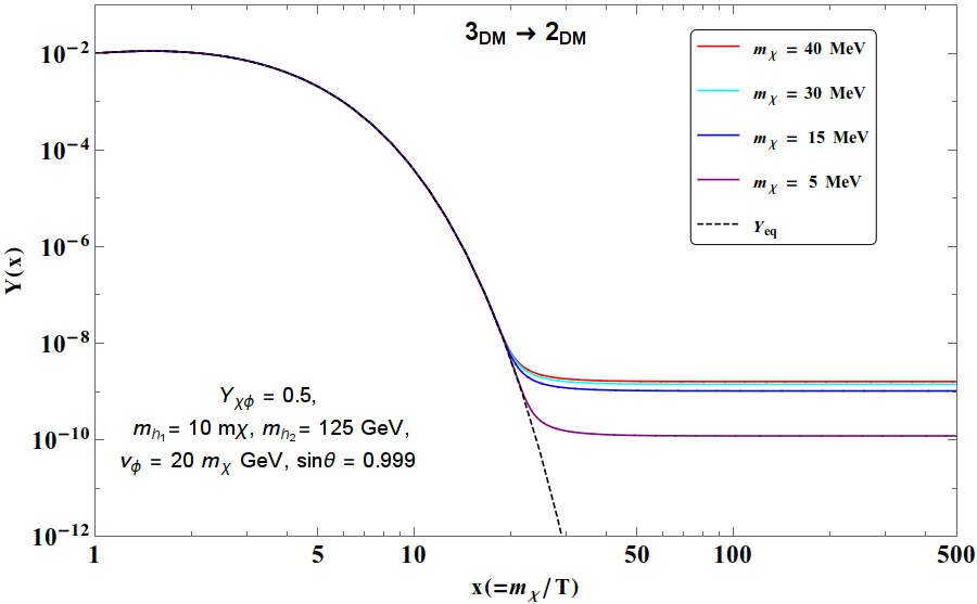
In Fig. 15, we demonstrate the freeze-out in such a case. In the top panel, we show the case when DM freeze-out through $3_{\rm{DM}}\to 2_{\rm{SM}}$ only (when only the second term is considered in BEQ 3.22). The solution shows that $3_{\rm{DM}}\to 2_{\rm{SM}}$ interaction is good enough to keep the DM follow equilibrium distribution at low $x$ and yields a typical but early freeze-out. On the bottom left panel, when we include additionally the annihilation through $3_{\rm{DM}}\to 2_{\rm{DM}}$ in the dark sector, due to enhanced self coupling (as chosen for the SIMP like case), the number changing process in the dark sector dominates over $3_{\rm{DM}}\to 2_{\rm{SM}}$ and yields a freeze-out that corresponds to correct relic. This is validated by taking $3_{\rm{DM}}\to 2_{\rm{DM}}$ annihilation in the dark sector only (as we have done for the analysis) in the bottom right panel to show that the freeze-out mimics the case of taking both contributions together (as in bottom left Fig. 15) and justifies our analysis.

3.6 $4_{\rm DM}\to 2_{\rm DM}$ SIMP scenario

SIMP like framework can also be realised when the dominant depletion in DM number density occurs through $4_{\rm DM}\to 2_{\rm DM}$ process as shown in the left hand side of Fig. 16. The BEQ for such a $4_{\rm DM}\to 2_{\rm DM}$ process is given by:

\displaystyle\frac{dY}{dx}=-0.0508~\frac{g_{*s}^{3}}{\sqrt{g_{*}}}~M_{Pl}~\frac{{m_{\rm DM}}^{7}}{x^{8}}~{\langle{\sigma v^{3}}\rangle}_{4_{\rm DM}\to 2_{\rm DM}}~\Big(Y^{4}-Y^{2}~Y_{eq}^{2}\Big),

(3.23)

where $g_{*s}=3.91$ and $g_{*}=3.36$ for KeV order DM. The freeze-out solution of BEQ in Eqn.3.23 in terms of $Y(=\frac{n}{s})$ is shown in RHS of Fig.16 with DM mass $26$ KeV for three different choices of $\langle{\sigma v^{3}}\rangle$ of $4_{\rm DM}\to 2_{\rm DM}$ cross-sections. We can see that correct relic density ( $\Omega h^{2}=0.12$ ) can be achieved when $\langle{\sigma v^{3}}\rangle\sim 10^{35}~{\rm GeV^{-8}}$ for $m_{DM}=26~{\rm KeV}$ in a model independent way.

In our model, $4_{\rm DM}\to 2_{\rm DM}$ processes occur through $\chi\chi^{*}\chi\chi^{*}\to\chi\chi$ and $\chi\chi\chi\chi\to\chi\chi^{*}$ mediated by $\chi,h_{1}$ and $h_{2}$ . The amplitude for such process therefore turns out to be:

\displaystyle|\mathcal{M}_{4_{\rm DM}\to 2_{\rm DM}}|^{2}=2\Big|\mathcal{M}_{\chi\chi^{*}\chi\chi^{*}\to\chi\chi}+\mathcal{M}_{\chi\chi\chi\chi\to\chi\chi^{*}}\Big|^{2},

(3.24)

where the factor of 2 comes from the corresponding conjugate processes. The thermal average of total cross section for $4_{\rm DM}\to 2_{\rm DM}$ processes is given by:

\displaystyle{\langle{\sigma v^{3}}\rangle}_{4_{\rm DM}\to 2_{\rm DM}}=\frac{\sqrt{3}}{256\pi m_{\chi}^{4}}|\mathcal{M}_{4_{\rm DM}\to 2_{\rm DM}}|^{2}.

(3.25)

The calculation of $\langle{\sigma v^{3}}\rangle$ for ${4_{\rm DM}\to 2_{\rm DM}}$ process is described in Appendix C. We however refrain from elaborating all the Feynman graphs that contribute to $\chi\chi^{*}\chi\chi^{*}\to\chi\chi$ and $\chi\chi\chi\chi\to\chi\chi^{*}$ in this model due to the large number of diagrams present.

We demonstrate freeze-out of $\chi$ through ${4_{\rm DM}\to 2_{\rm DM}}$ process in Fig. 17 in $Y-x$ plane for $m_{\chi}=26$ KeV in our model. We choose three values of $Y_{\chi\phi}$ for demonstration. The one corresponds to correct relic is given by $Y_{\chi\phi}=5\times 10^{-9}$ , with other parameters kept fixed and mentioned in figure inset. It is clear that the correct density obtained by a DM mass so light ( $\sim$ $\mathcal{O}$ (KeV) ), already has compensated for the phase space suppression and therefore do not require a coupling in strong limit. With larger DM mass, the coupling gets larger. However, the required couplings to satisfy correct relic density for KeV order DM are much smaller compared to MeV order SIMP mass. Therefore, automatically due to the choices of parameters made above, $3_{\rm DM}\to 2_{\rm DM}$ number changing processes are suppressed and the freeze-out is governed by $4_{\rm DM}\to 2_{\rm DM}$ .

4 WIMP realisation of the model

Finally for comparison, we demonstrate the WIMP realisation of the same model that we have studied in this paper. The BEQ in WIMP scenario is given by:

	$\displaystyle\frac{dY}{dx}$	$\displaystyle=$	$\displaystyle-0.264g_{s}^{1/2}~M_{pl}~\frac{m_{\chi}}{x^{2}}\langle\sigma v\rangle_{2_{\rm DM}\to 2_{\rm SM}}\Big(Y^{2}-Y_{eq}^{2}\Big)$		(4.1)
			$\displaystyle-0.115g_{s}^{3/2}~M_{pl}~\frac{m_{\chi}^{4}}{x^{5}}~\langle\sigma v^{2}\rangle_{3_{\rm DM}\to 2_{\rm DM}}\Big(Y^{3}-Y^{2}Y_{eq}\Big).$		(4.1)

In the above Eqn. 4.1, we have considered the DM annihilation to SM through $2_{\rm DM}\to 2_{\rm SM}$ and also the one used for SIMP condition, namely $3_{\rm DM}\to 2_{\rm DM}$ process. DM freeze-out is shown in Fig. 18 for three cases: (i) considering only $2_{\rm DM}\to 2_{\rm SM}$ (blue line), (ii) only $3_{\rm DM}\to 2_{\rm DM}$ (cyan line), (iii) the actual situation $2_{\rm DM}\to 2_{\rm SM}$ and $3_{\rm DM}\to 2_{\rm DM}$ together (red dashed) following Eqn. 4.1. We clearly see here that $3_{\rm DM}\to 2_{\rm DM}$ annihilation has a very small contribution as the lone process of such kind will yield an early freeze-out, whereas when considered together with $2_{\rm DM}\to 2_{\rm SM}$ , can not be distinguished from the case (iii) where $2_{\rm DM}\to 2_{\rm SM}$ and $3_{\rm DM}\to 2_{\rm DM}$ are addressed together. Therefore, it is quite justified to neglect the second term in BEQ 4.1 for WIMP solution.

As has already been mentioned that SIMP realisation of this model was possible by choosing the coupling to SM very feeble, namely keeping $\lambda_{\chi\phi}=\lambda_{\chi h}\sim 0.001$ , altering which the $2_{\rm DM}\to 2_{\rm SM}$ annihilation to SM dominates over the $3_{\rm DM}\to 2_{\rm DM}$ in dark sector and governs the freeze-out to reveal WIMP paradigm of the model. We show next the variation in relic density with DM mass in Fig. 19 for WIMP realisation of the model. We choose to illustrate two different values of the additional scalar boson mass: a light scalar mass of 80 GeV for the left plot and a heavy scalar of 400 GeV in the right plot. To compute relic density and direct search cross section for the model we have used micrOmegas [51]. We see that two resonance drops at $m_{h_{1,2}}/2$ are clearly observed for s-channel mediation of $h_{1,2}$ in $2_{\rm DM}\to 2_{\rm SM}$ annihilation process. We also point out the variation in $\mu_{\chi}$ for illustration, the larger the $\mu_{\chi}$ , the larger is the annihilation cross-section and therefore smaller is the relic density. There exist a semi-annihilation effect $\chi\chi\to h\chi$ for the WIMP DM here that helps disentangling the relic density to direct search; but, to drop below the direct search constraints require a large $\mu_{\chi}$ , that lies in tension with vacuum stability.

We next analyse the constraint coming from direct search to the relic density allowed parameter space of the WIMP scenario of the model. The Feynman graph for direct search interaction is shown in Fig. 20 through t-channel $h_{1,2}$ mediation. The scan for relic density allowed parameter space of the model in spin independent direct search cross section versus DM mass plane is shown in Fig. 21. We have chosen two different possible phenomenological situations for illustration: light additional scalar ( $m_{h_{1}}=40$ GeV in blue and $m_{h_{1}}=80$ GeV in golden yellow) on the left panel and heavy scalar ( $m_{h_{2}}=400$ GeV) on the right panel. The main outcome of this analysis is to see that immaterial to the additional scalar mass resonance regions are allowed by direct search. Interestingly, when the additional scalar mass is not too far from the SM Higgs, as is the case for $m_{h_{1}}=80$ GeV as shown by golden yellow points in the left panel, there is a large region of heavy DM mass ( $\sim 800\to 1000$ GeV), which becomes allowed by direct search constraint. This can be explained by realizing that since the spin independent direct search cross-section follows [45]:

\sigma_{\rm DD}^{\rm SI}=\frac{1}{4\pi}\bigg(\frac{f_{n}\mu_{n}}{m_{\chi}}\bigg)^{2}\bigg(\frac{m_{n}}{v_{h}}\bigg)^{2}\bigg[\frac{\lambda_{a1}\cos\theta}{m_{h_{1}}^{2}}+\frac{\lambda_{b1}\sin\theta}{m_{h_{2}^{2}}}\bigg]^{2}~,

(4.2)

where $\lambda_{a1}$ and $\lambda_{b1}$ are DM-Higgs coupling, $f_{n}$ is the form factor, $\mu_{n}=m_{n}m_{\chi}/(m_{n}+m_{\chi})$ is the reduced mass. The cross-section yields a destructive interference due to opposite sign of $\lambda_{a1}$ and $\lambda_{b1}$ (look at the Table 2 of vertices in Appendix A) when the two scalar masses are close.

5 Summary and Conclusion

We have presented a model where both SIMP and WIMP realization of a scalar DM is possible. This is achieved by assuming a complex scalar field $\chi$ which transforms under unbroken $\mathcal{Z}_{3}$ . When the portal coupling is small, it provides a SIMP solution and when the portal coupling is large, it provides a WIMP like solution. In principle, this bit of model construct is good enough to realise the correct relic density in SIMP scenario and perhaps serves as the simplest SIMP DM, where the number changing process within the dark sector is solely governed by DM self coupling. However, we add to that another scalar field $\phi$ that is even under $\mathcal{Z}_{3}$ , acquires a vev, mixes with SM Higgs and serves as a light scalar mediator to aid DM self scattering to yield a large parameter space available to the model. We also see that due to the presence of this additional field, the self coupling to achieve a successful SIMP DM paradigm enjoys a larger freedom. The allowed parameter space gets further restricted from the self scattering constraints and unitarity bound; for Bullet cluster the bound turns out to be within $\sim 200$ MeV, while for Abell cluster data, the bound is more restrictive and remains within $\sim 50$ MeV.

The model can also serve a successful freeze-out through $4_{\rm DM}\to 2_{\rm DM}$ number changing processes, and achieve correct relic density for DM mass $\sim$ $\mathcal{O}({\rm KeV})$ , where the couplings required are much smaller than that of $3_{\rm DM}\to 2_{\rm DM}$ case, automatically justifying the suppression of $3_{\rm DM}\to 2_{\rm DM}$ processes in such circumstances.

The condition to keep the DM in thermal equilibrium at early universe and not heating up through the number changing processes within the dark sector, have been verified for points satisfying correct relic density. Additionally, we have verified the kinetic interaction of DM with SM remains larger than the Hubble expansion rate before freeze-out.

We also analyse the WIMP limit of the DM for the sake of comparison. Interestingly the direct search allowed parameter space for such a framework predict that the additional Higgs mass should be close to the SM Higgs due to a destructive interference in the direct search cross-section. On the other hand SIMP realisation is aided when the additional scalar is light of the order of sub-GeV. It is important to remind that such a scalar is quite likely to evade the collider search bound due to its singlet nature.

Thermal freeze out of the DM in SIMP condition for $3_{\rm DM}\to 2_{\rm DM}$ number changing process is performed in details and we advocate an approximate analytical solution for relic density which yields agreement to the numerical solution for a certain range of DM mass. We also calculate all the cross-sections for freeze out and self scattering in details, so that the draft serves as a useful reference for performing phenomenological analysis in any SIMP framework.

Acknowledgement

SV acknowledges to the BTP project at the department of Physics in IIT Guwahati, where the project was initiated. SB and SV also acknowledges DST-INSPIRE Faculty grant IFA-13 PH-57. PG would like to thank MHRD, Government of India for research fellowship.

Appendix

Appendix A Vertices and Couplings of the model

Here we list all the vertices that appear in the cross-sections for annihilation and scattering processes in this model. We also introduce a shorthand notation for each vertex that will be used further in computing the amplitudes.

Vertices	Vertex factor	Notation
$\chi^{}\chi\chi^{}\chi$	$-(2!2!)\>\lambda_{\chi}=\>-4\lambda_{\chi}$	$-\lambda_{4}$
$\chi\chi\chi$	$-\frac{(\mu_{\chi}+Y_{\chi\phi}v_{\phi})}{6}3!=-(\mu_{\chi}+Y_{\chi\phi}v_{\phi})$	$-\lambda_{3}$
$\chi^{*}\chi h_{1}$	$-(\lambda_{\chi h}v_{h}\cos\theta-(\lambda_{\chi\phi}v_{\phi}+\mu_{\chi\phi})\sin\theta)$	$-\lambda_{a1}$
$\chi^{*}\chi h_{2}$	$-(\lambda_{\chi h}v_{h}\sin\theta+(\lambda_{\chi\phi}v_{\phi}+\mu_{\chi\phi})\cos\theta)$	$-\lambda_{b1}$
$\chi\chi\chi h_{1}$	$-(-\sin\theta Y_{\chi\phi})$	$-\lambda_{a2}$
$\chi\chi\chi h_{2}$	$-(-\cos\theta Y_{\chi\phi})$	$-\lambda_{b2}$
$f\bar{f}h_{1}$	$-\frac{m_{f}}{v}\cos\theta$	$-\lambda_{f1}$
$f\bar{f}h_{2}$	$-\frac{m_{f}}{v}\sin\theta$	$-\lambda_{f2}$
$h_{1}h_{1}h_{1}$	$3\cos\theta\sin\theta[\cos\theta(v_{\phi}\lambda_{\phi h}+\mu_{\phi h})-\sin\theta(\lambda_{\phi h}v_{h})]$	$-\lambda_{H1}$
	$+6\sin^{3}\theta v_{\phi}\lambda_{\phi}-6\cos^{3}\theta v_{h}\lambda_{h}-2\sin\theta\mu_{3}$
$\chi\chi^{*}h_{1}h_{1}$	$-\cos^{2}\theta\lambda_{\chi h}-\sin^{2}\theta\lambda_{\chi\phi}$	$-\lambda_{\chi H1}$

Table 2: Couplings (in terms of the model parameters, see Eq. 3.3) that appear in the model and is required for computing all the processes considered in this analysis. Shorthand notations are introduced.

Appendix B Annihilation cross-section for $3_{{\textrm{DM}}}\to 2_{{\textrm{DM}}}$ process

We first note that the dominant contribution in absence of $2_{\rm DM}\to 2_{\rm SM}$ annihilations to SM are $3_{{\textrm{DM}}}\to 2_{{\textrm{DM}}}$ that yields the required freeze out. Apart from $\chi$ mediation, the two other mediators for such diagrams are the two Higgses, which are mentioned by the following notation in the matrix element :

	$\displaystyle a\Rightarrow h_{1}\>\textrm{mediation}~,$
	$\displaystyle b\Rightarrow h_{2}\>\textrm{mediation}~.$

There are two major processes in the model which contribute to such case: $\chi\chi\chi\to\chi\chi^{*}$ and $\chi\chi^{*}\chi^{*}\to\chi\chi$ and their conjugates. We will analyse them systematically below.

$\chi\chi\chi\to\chi\chi^{*}$

Feynman Diagrams

Matrix Amplitude

Only $h_{1,2}$ mediated

•

$\mathcal{M}_{1a}=\frac{(-\lambda_{a1})(-\lambda_{a2})}{s-m_{h_{1}}^{2}}$
•

$\mathcal{M}_{2a}=\frac{(-\lambda_{a1})(-\lambda_{a2})}{t-m_{h_{1}}^{2}}$
•

$\mathcal{M}_{1b}=\frac{(-\lambda_{b1})(-\lambda_{b2})}{s-m_{h_{2}}^{2}}$
•

$\mathcal{M}_{2b}=\frac{(-\lambda_{b1})(-\lambda_{b2})}{t-m_{h_{2}}^{2}}$

$h_{1,2}$ and $\chi$ mediated

•

$\mathcal{M}_{3a}=\frac{(-\lambda_{a1})^{2}(-\lambda_{3})}{(s-m_{h_{1}}^{2})(t-m_{\chi}^{2})}$
•

$\mathcal{M}_{4a}=\frac{(-\lambda_{a1})^{2}(-\lambda_{3})}{(t-m_{h_{1}}^{2})(s-m_{\chi}^{2})}$
•

$\mathcal{M}_{5a}=\frac{(-\lambda_{a1})^{2}(-\lambda_{3})}{(t-m_{h_{1}}^{2})(t-m_{\chi}^{2})}$
•

$\mathcal{M}_{3b}=\frac{(-\lambda_{b1})^{2}(-\lambda_{3})}{(s-m_{h_{2}}^{2})(t-m_{\chi}^{2})}$
•

$\mathcal{M}_{4b}=\frac{(-\lambda_{b1})^{2}(-\lambda_{3})}{(t-m_{h_{2}}^{2})(s-m_{\chi}^{2})}$
•

$\mathcal{M}_{5b}=\frac{(-\lambda_{b1})^{2}(-\lambda_{3})}{(t-m_{h_{2}}^{2})(t-m_{\chi}^{2})}$

Only $\chi$ mediated

•

$\mathcal{M}_{6}=\frac{(-\lambda_{3})(-\lambda_{4})}{s-m_{\chi}^{2}}$
•

$\mathcal{M}_{7}=\frac{(-\lambda_{3})(-\lambda_{4})}{t-m_{\chi}^{2}}$
•

$\mathcal{M}_{8}=\frac{(-\lambda_{3})^{3}}{(s-m_{\chi}^{2})(t-m_{\chi}^{2})}$

	$\displaystyle\mathcal{M}_{Net}$	$\displaystyle=$	$\displaystyle(\mathcal{M}_{1a}+\mathcal{M}_{2a}+\mathcal{M}_{3a}+\mathcal{M}_{4a}+\mathcal{M}_{5a})+(\mathcal{M}_{1b}+\mathcal{M}_{2b}+\mathcal{M}_{3b}+\mathcal{M}_{4b}+\mathcal{M}_{5b})$
			$\displaystyle+\mathcal{M}_{6}+\mathcal{M}_{7}+\mathcal{M}_{8}$

Matrix amplitude squared is then

\Rightarrow|\mathcal{M}_{\chi\chi\chi\to\chi\chi^{*}}|^{2}=|\mathcal{M}_{Net}|^{2}.

The complex conjugate of $\chi\chi\chi\to\chi\chi^{*}$ $i.e.$ $\chi^{*}\chi^{*}\chi^{*}\to\chi^{*}\chi$ also contributes to the total matrix amplitude and has same expression as $\chi\chi\chi\to\chi\chi^{*}$ ,

|\mathcal{M}_{\chi\chi\chi\to\chi\chi^{*}}|^{2}=|\mathcal{M}_{\chi^{*}\chi^{*}\chi^{*}\to\chi^{*}\chi}|^{2}.

Therefore the thermal average cross-section reads:

	$\displaystyle\langle\sigma_{\chi\chi\chi\to\chi\chi^{*}}v^{2}\rangle$	$\displaystyle=$	$\displaystyle\frac{\sqrt{5}}{192\pi m_{\chi}^{3}}\bigg[\|\mathcal{M}_{\chi\chi\chi\to\chi\chi^{}}\|^{2}+\|\mathcal{M}_{\chi^{}\chi^{}\chi^{}\to\chi^{*}\chi}\|^{2}\bigg]$		(B.1)
		$\displaystyle=$	$\displaystyle\frac{\sqrt{5}}{192\pi m_{\chi}^{3}}\bigg[2\times\|\mathcal{M}_{\chi\chi\chi\to\chi\chi^{*}}\|^{2}\bigg].$		(B.1)

We will derive the last expression in a moment. $\chi\chi^{*}\chi^{*}\to\chi\chi$

Feynman Diagrams

Note here that we have not shown $u$ -channel graphs, which will also contribute to the cross-section.

Matrix Amplitude

Only $\chi$ mediated

•

$\mathcal{M}_{11}=\frac{(-\lambda_{3})(-\lambda_{4})}{s-m_{\chi}^{2}}$
•

$\mathcal{M}_{12}=\frac{(-\lambda_{3})^{3}}{(s-m_{\chi}^{2})(t-m_{\chi}^{2})}$
•

$\mathcal{M}_{13}=\frac{(-\lambda_{3})(-\lambda_{4})}{t-m_{\chi}^{2}}$
•

$\mathcal{M}_{14}=\frac{(-\lambda_{3})(-\lambda_{4})}{s-m_{\chi}^{2}}$

•

$\mathcal{M}_{15t}=\frac{(-\lambda_{3})^{3}}{(t-m_{\chi}^{2})(t-m_{\chi}^{2})}$
•

$\mathcal{M}_{15u}=\frac{(-\lambda_{3})^{3}}{(u-m_{\chi}^{2})(t-m_{\chi}^{2})}$
•

$\mathcal{M}_{16t}=\frac{(-\lambda_{3})(-\lambda_{4})}{t-m_{\chi}^{2}}$
•

$\mathcal{M}_{16u}=\frac{(-\lambda_{3})(-\lambda_{4})}{u-m_{\chi}^{2}}$

Only $h_{1,2}$ mediated,

•

$\mathcal{M}_{1at}=\frac{(-\lambda_{a1})(-\lambda_{a2})}{t-m_{h_{1}}^{2}}$
•

$\mathcal{M}_{1au}=\frac{(-\lambda_{a1})(-\lambda_{a2})}{u-m_{h_{1}}^{2}}$
•

$\mathcal{M}_{2at}=\frac{(-\lambda_{a1})(-\lambda_{a2})}{t-m_{h_{1}}^{2}}$
•

$\mathcal{M}_{2au}=\frac{(-\lambda_{a1})(-\lambda_{a2})}{u-m_{h_{1}}^{2}}$
•

$\mathcal{M}_{3a}=\frac{(-\lambda_{a1})(-\lambda_{a2})}{t-m_{h_{1}}^{2}}$
•

$\mathcal{M}_{1bt}=\frac{(-\lambda_{a1})(-\lambda_{a2})}{t-m_{h_{2}}^{2}}$
•

$\mathcal{M}_{1bu}=\frac{(-\lambda_{a1})(-\lambda_{a2})}{u-m_{h_{2}}^{2}}$
•

$\mathcal{M}_{2bt}=\frac{(-\lambda_{a1})(-\lambda_{a2})}{t-m_{h_{2}}^{2}}$
•

$\mathcal{M}_{2bu}=\frac{(-\lambda_{a1})(-\lambda_{a2})}{u-m_{h_{2}}^{2}}$
•

$\mathcal{M}_{3b}=\frac{(-\lambda_{a1})(-\lambda_{a2})}{t-m_{h_{2}}^{2}}$

$h_{1}$ and $\chi$ mediated

•

$\mathcal{M}_{4at}=\frac{(-\lambda_{a1})^{2}(-\lambda_{3})}{(t-m_{h_{1}}^{2})(s-m_{\chi}^{2})}$
•

$\mathcal{M}_{4au}=\frac{(-\lambda_{a1})^{2}(-\lambda_{3})}{(u-m_{h_{1}}^{2})(s-m_{\chi}^{2})}$
•

$\mathcal{M}_{5at}=\frac{(-\lambda_{a1})^{2}(-\lambda_{3})}{(s-m_{h_{1}}^{2})(t-m_{\chi}^{2})}$
•

$\mathcal{M}_{5au}=\frac{(-\lambda_{a1})^{2}(-\lambda_{3})}{(s-m_{h_{1}}^{2})(-m_{\chi}^{2})}$
•

$\mathcal{M}_{6at}=\frac{(-\lambda_{a1})^{2}(-\lambda_{3})}{(t-m_{h_{1}}^{2})(s-m_{\chi}^{2})}$
•

$\mathcal{M}_{6au}=\frac{(-\lambda_{a1})^{2}(-\lambda_{3})}{(u-m_{h_{1}}^{2})(s-m_{\chi}^{2})}$
•

$\mathcal{M}_{7at}=\frac{(-\lambda_{a1})^{2}(-\lambda_{3})}{(t-m_{h_{1}}^{2})(t-m_{\chi}^{2})}$
•

$\mathcal{M}_{7au}=\frac{(-\lambda_{a1})^{2}(-\lambda_{3})}{(s-m_{h_{1}}^{2})(u-m_{\chi}^{2})}$
•

$\mathcal{M}_{8a}=\frac{(-\lambda_{a1})^{2}(-\lambda_{3})}{(t-m_{h_{1}}^{2})(s-m_{\chi}^{2})}$
•

$\mathcal{M}_{9at}=\frac{(-\lambda_{a1})^{2}(-\lambda_{3})}{(t-m_{h_{1}}^{2})(t-m_{\chi}^{2})}$
•

$\mathcal{M}_{9au}=\frac{(-\lambda_{a1})^{2}(-\lambda_{3})}{(s-m_{h_{1}}^{2})(u-m_{\chi}^{2})}$
•

$\mathcal{M}_{10at}=\frac{(-\lambda_{a1})^{2}(-\lambda_{3})}{(s-m_{h_{1}}^{2})(t-m_{\chi}^{2})}$
•

$\mathcal{M}_{10au}=\frac{(-\lambda_{a1})^{2}(-\lambda_{3})}{(s-m_{h_{1}}^{2})(u-m_{\chi}^{2})}$

$h_{2}$ and $\chi$ mediated

•

$\mathcal{M}_{4bt}=\frac{(-\lambda_{b1})^{2}(-\lambda_{3})}{(t-m_{h_{1}}^{2})(s-m_{\chi}^{2})}$
•

$\mathcal{M}_{4bu}=\frac{(-\lambda_{b1})^{2}(-\lambda_{3})}{(u-m_{h_{1}}^{2})(s-m_{\chi}^{2})}$
•

$\mathcal{M}_{5bt}=\frac{(-\lambda_{b1})^{2}(-\lambda_{3})}{(s-m_{h_{1}}^{2})(t-m_{\chi}^{2})}$
•

$\mathcal{M}_{5b}=\frac{(-\lambda_{b1})^{2}(-\lambda_{3})}{(s-m_{h_{1}}^{2})(u-m_{\chi}^{2})}$
•

$\mathcal{M}_{6bt}=\frac{(-\lambda_{b1})^{2}(-\lambda_{3})}{(t-m_{h_{1}}^{2})(s-m_{\chi}^{2})}$
•

$\mathcal{M}_{6bu}=\frac{(-\lambda_{b1})^{2}(-\lambda_{3})}{(u-m_{h_{1}}^{2})(s-m_{\chi}^{2})}$
•

$\mathcal{M}_{7bt}=\frac{(-\lambda_{b1})^{2}(-\lambda_{3})}{(t-m_{h_{1}}^{2})(t-m_{\chi}^{2})}$
•

$\mathcal{M}_{7bu}=\frac{(-\lambda_{b1})^{2}(-\lambda_{3})}{(u-m_{h_{1}}^{2})(t-m_{\chi}^{2})}$
•

$\mathcal{M}_{8b}=\frac{(-\lambda_{b1})^{2}(-\lambda_{3})}{(t-m_{h_{2}}^{2})(s-m_{\chi}^{2})}$
•

$\mathcal{M}_{9bt}=\frac{(-\lambda_{b1})^{2}(-\lambda_{3})}{(t-m_{h_{2}}^{2})(t-m_{\chi}^{2})}$
•

$\mathcal{M}_{9bu}=\frac{(-\lambda_{b1})^{2}(-\lambda_{3})}{(u-m_{h_{2}}^{2})(t-m_{\chi}^{2})}$
•

$\mathcal{M}_{10bt}=\frac{(-\lambda_{b1})^{2}(-\lambda_{3})}{(s-m_{h_{2}}^{2})(t-m_{\chi}^{2})}$
•

$\mathcal{M}_{10bt}=\frac{(-\lambda_{b1})^{2}(-\lambda_{3})}{(s-m_{h_{2}}^{2})(u-m_{\chi}^{2})}$

	$\displaystyle\mathcal{M}_{net}=$	$\displaystyle(\mathcal{M}_{1at}+\mathcal{M}_{1au}+\mathcal{M}_{2at}\mathcal{M}_{2au}+\mathcal{M}_{3a}+\mathcal{M}_{4at}+\mathcal{M}_{4au}+\mathcal{M}_{5at}+\mathcal{M}_{5au}$
		$\displaystyle+\mathcal{M}_{6at}+\mathcal{M}_{6au}+\mathcal{M}_{7at}+\mathcal{M}_{7au}+\mathcal{M}_{8a}+\mathcal{M}_{9at}+\mathcal{M}_{9au}+\mathcal{M}_{10at}+\mathcal{M}_{10au})$
		$\displaystyle+(\mathcal{M}_{1bt}+\mathcal{M}_{1bu}+\mathcal{M}_{2bt}+\mathcal{M}_{2bu}+\mathcal{M}_{3b}+\mathcal{M}_{4bt}+\mathcal{M}_{4bu}+\mathcal{M}_{5bt}+\mathcal{M}_{5bu}$
		$\displaystyle+\mathcal{M}_{6bt}+\mathcal{M}_{6bu}+\mathcal{M}_{7bt}+\mathcal{M}_{7bu}+\mathcal{M}_{8b}+\mathcal{M}_{9bt}+\mathcal{M}_{9bu}+\mathcal{M}_{10bt}+\mathcal{M}_{10bu})$
		$\displaystyle+(\mathcal{M}_{11}+\mathcal{M}_{12}+\mathcal{M}_{13}+\mathcal{M}_{14}+\mathcal{M}_{15t}+\mathcal{M}_{15u}+\mathcal{M}_{16t}+\mathcal{M}_{16u})$

Note above that we have written the u-channel contribution also, which exists corresponding to each t-channel graph as the final state particles here are identical. Squared matrix amplitude is given as,

\Rightarrow|\mathcal{M}_{\chi\chi^{*}\chi^{*}\to\chi\chi}|^{2}=\frac{1}{2}|\mathcal{M}_{net}|^{2}.

The complex conjugate of $\chi\chi^{*}\chi^{*}\to\chi\chi$ $i.e.$ $\chi^{*}\chi\chi\to\chi^{*}\chi^{*}$ also contributes to the total matrix amplitude and has same expression as $\chi\chi^{*}\chi^{*}\to\chi\chi$ ,

|\mathcal{M}_{\chi\chi^{*}\chi^{*}\to\chi\chi}|^{2}=|\mathcal{M}_{\chi^{*}\chi\chi\to\chi^{*}\chi^{*}}|^{2}.

The thermal average cross-section reads:

	$\displaystyle\langle\sigma_{\chi\chi^{}\chi^{}\to\chi\chi}v^{2}\rangle$	$\displaystyle=$	$\displaystyle\frac{\sqrt{5}}{192\pi m_{\chi}^{3}}\bigg[\|\mathcal{M}_{\chi\chi^{}\chi^{}\to\chi\chi}\|^{2}+\|\mathcal{M}_{\chi^{}\chi\chi\to\chi^{}\chi^{*}}\|^{2}\bigg]$		(B.2)
		$\displaystyle=$	$\displaystyle\frac{\sqrt{5}}{192\pi m_{\chi}^{3}}\bigg[2\times\|\mathcal{M}_{\chi\chi^{}\chi^{}\to\chi\chi}\|^{2}\bigg]~.$		(B.2)

Therefore, the total thermal average cross section for $3_{{\textrm{DM}}}\to 2_{{\textrm{DM}}}$ process turn out to be:

	$\displaystyle\langle\sigma_{3_{{\textrm{DM}}}\to 2_{{\textrm{DM}}}}v^{2}\rangle$	$\displaystyle=$	$\displaystyle\langle\sigma_{\chi\chi\chi\to\chi\chi^{}}v^{2}\rangle+\langle\sigma_{\chi\chi^{}\chi^{*}\to\chi\chi}v^{2}\rangle$		(B.3)
		$\displaystyle=$	$\displaystyle\frac{\sqrt{5}}{192\pi m_{\chi}^{3}}\bigg[2\times\bigg(\|\mathcal{M}_{\chi\chi\chi\to\chi\chi^{}}\|^{2}+\|\mathcal{M}_{\chi\chi^{}\chi^{*}\to\chi\chi}\|^{2}\bigg)\bigg].$		(B.3)

General expression for $3_{\textrm{DM}}\to 2_{\textrm{DM}}$ annihilation cross-section

Let us derive the $3_{{\textrm{DM}}}\to 2_{{\textrm{DM}}}$ annihilation cross-section in a model independent way as a function of the amplitude. We consider a process like:

\displaystyle\chi(p_{1})~\chi(p_{2})~\chi(p_{3})~\to~\chi(p_{4})~\chi(p_{5})~~.

In non-relativistic limit,

	$\displaystyle E_{1}=E_{2}=E_{3}$	$\displaystyle=$	$\displaystyle m_{\chi}$
	$\displaystyle\Rightarrow E_{1}+E_{2}+E_{3}$	$\displaystyle=$	$\displaystyle 3m_{\chi}.$		(B.4)

$P_{i=1-5}$ are the three-momentum of incoming and outgoing particles. Now, one can express $(\sigma v^{2})_{3_{DM}\to 2_{DM}}$ as [32]:

$\displaystyle(\sigma v^{2})_{3_{\rm DM}\to 2_{\rm DM}}$	$\displaystyle=$	$\displaystyle\frac{1}{(2E_{1})(2E_{2})(2E_{3})}\int\frac{d^{3}P_{4}}{(2\pi)^{3}2E_{4}}\frac{d^{3}P_{5}}{(2\pi)^{3}2E_{5}}(2\pi)^{4}\delta^{4}(p_{1}+p_{2}+p_{3}-p_{4}-p_{5})\|\mathcal{M}\|_{3\to 2}^{2}$	(B.5)
	$\displaystyle=$	$\displaystyle\frac{1}{(2E_{1})(2E_{2})(2E_{3})}\frac{\|\mathcal{M}\|_{3\to 2}^{2}}{(2\pi)^{6}}\int\frac{d^{3}P_{4}}{2E_{4}}\frac{d^{3}P_{5}}{2E_{5}}(2\pi)^{4}\delta(E_{1}+E_{2}+E_{3}-E_{4}-E_{5})$
		$\displaystyle\hskip 213.39566pt\delta^{3}(P_{1}+P_{2}+P_{3}-P_{4}-P_{5}),$

assuming that the matrix amplitude is independent of the final outgoing particles. Now, in the centre of mass frame $P_{1}+P_{2}+P_{3}=0$ , leads to:

\displaystyle(\sigma v^{2})_{3_{\rm DM}\to 2_{\rm DM}}

\displaystyle=

\displaystyle\frac{1}{(2E_{1})(2E_{2})(2E_{3})}\frac{|\mathcal{M}|_{3\to 2}^{2}}{(2\pi)^{2}}\int\frac{d^{3}P_{4}}{2E_{4}}\frac{d^{3}P_{5}}{2E_{5}}\delta(E_{1}+E_{2}+E_{3}-E_{4}-E_{5})\delta^{3}(P_{4}+P_{5}).

Using Eq.(B) and the delta function gives us: $P_{4}=-P_{5}$ . We also know that $E_{5}=\sqrt{P_{5}^{2}+m_{\chi}^{2}}$ . So integrating over $P_{5}$ we get :

$\displaystyle(\sigma v^{2})_{3_{\rm DM}\to 2_{\rm DM}}$	$\displaystyle=$	$\displaystyle\frac{1}{8m_{\chi}^{3}}\frac{\|\mathcal{M}\|_{3\to 2}^{2}}{(2\pi)^{2}}\int\frac{d^{3}P_{4}}{2E_{4}}\frac{1}{2\sqrt{P_{4}^{2}+m_{\chi}^{2}}}\delta(3m_{\chi}-2\sqrt{P_{4}^{2}+m_{\chi}^{2}})$
	$\displaystyle=$	$\displaystyle\frac{1}{8m_{\chi}^{3}}\frac{\|\mathcal{M}\|_{3\to 2}^{2}}{(2\pi)^{2}}\int\frac{P_{4}^{2}dP_{4}d\Omega}{4(P_{4}^{2}+m_{\chi}^{2})}\delta(3m_{\chi}-2\sqrt{P_{4}^{2}+m_{\chi}^{2}})$
	$\displaystyle=$	$\displaystyle\frac{1}{8m_{\chi}^{3}}\frac{\|\mathcal{M}\|_{3\to 2}^{2}}{(2\pi)^{2}}\frac{4\pi}{4}\int\frac{P_{4}^{2}dP_{4}}{(P_{4}^{2}+m_{\chi}^{2})}\delta(3m_{\chi}-2\sqrt{P_{4}^{2}+m_{\chi}^{2}})$
	$\displaystyle=$	$\displaystyle\frac{1}{8m_{\chi}^{3}}\frac{\|\mathcal{M}\|_{3\to 2}^{2}}{4\pi}\int\frac{P_{4}^{2}dP_{4}}{(P_{4}^{2}+m_{\chi}^{2})}\delta(3m_{\chi}-2\sqrt{P_{4}^{2}+m_{\chi}^{2}})$
	$\displaystyle=$	$\displaystyle\frac{1}{2\times 32\pi m_{\chi}^{3}}\|\mathcal{M}\|_{3\to 2}^{2}\int\frac{P_{4}^{2}dP_{4}}{(P_{4}^{2}+m_{\chi}^{2})}\delta(\frac{3}{2}m_{\chi}-\sqrt{P_{4}^{2}+m_{\chi}^{2}}).$

Finally integrating over $P_{4}$ we get,

\displaystyle(\sigma v^{2})_{3_{\rm DM}\to 2_{\rm DM}}

\displaystyle=

\displaystyle\frac{\sqrt{5}}{3}\times\frac{1}{64\pi m_{\chi}^{3}}|\mathcal{M}|_{3\to 2}^{2}~.

(B.6)

The thermal averaged cross section under the conditions mentioned above can be written as,

	$\displaystyle\langle\sigma v^{2}\rangle_{3_{\rm DM}\to 2_{\rm DM}}$	$\displaystyle=$	$\displaystyle\frac{1}{n_{1}^{eq}~n_{2}^{eq}~n_{3}^{eq}}\int\frac{g_{DM}~d^{3}P_{1}}{(2\pi)^{3}2E_{1}}~\frac{g_{DM}~d^{3}P_{2}}{(2\pi)^{3}2E_{2}}~\frac{g_{DM}~d^{3}P_{3}}{(2\pi)^{3}2E_{3}}~\frac{g_{DM}~d^{3}P_{4}}{(2\pi)^{3}2E_{4}}~\frac{g_{DM}~d^{3}P_{5}}{(2\pi)^{3}2E_{5}}$		(B.7)
			$\displaystyle~~~~~~~~~(2\pi)^{4}\delta^{4}(p_{1}+p_{2}+p_{3}-p_{4}-p_{5})\times\|\mathcal{M}_{3\to 2}\|^{2}~f_{1}^{eq}f_{2}^{eq}f_{3}^{eq}~~.$		(B.7)

Using Eq.(B.5) and Eq.(B.7), we can write,

\displaystyle\langle\sigma v^{2}\rangle_{3_{\rm DM}\to 2_{\rm DM}}

\displaystyle=

\displaystyle\frac{1}{n_{1}^{eq}~n_{2}^{eq}~n_{3}^{eq}}\int\frac{g_{DM}~d^{3}P_{1}}{(2\pi)^{3}}~\frac{g_{DM}\>d^{3}P_{2}}{(2\pi)^{3}}~\frac{g_{DM}~d^{3}P_{3}}{(2\pi)^{3}}~f_{1}^{eq}f_{2}^{eq}f_{3}^{eq}~(\sigma v^{2})_{3_{DM}\to 2_{DM}}~,

where $n_{i}^{eq}$ can be expressed in terms of modified Bessel’s function as [38],

\displaystyle n_{i}^{eq}=\frac{g_{DM}}{(2\pi)^{3}}\int d^{3}P_{i}~f^{eq}(E_{i},T)~.

(B.9)

Since,

$\displaystyle d^{3}P_{i}~f^{eq}(E_{i},T)$	$\displaystyle=$	$\displaystyle 4\pi m_{\chi}^{3}\bigg(\frac{E_{i}}{m_{\chi}}\bigg)~\bigg(\sqrt{\bigg(\frac{E_{i}}{m_{\chi}}\bigg)^{2}-1}\bigg)~e^{-(\frac{E_{i}}{m_{\chi}})(\frac{m_{\chi}}{T})}d\bigg(\frac{E_{i}}{m_{\chi}}\bigg),$
$\displaystyle\implies\int d^{3}P_{i}~f^{eq}(E_{i},T)$	$\displaystyle=$	$\displaystyle 4\pi m_{\chi}^{3}\int\bigg(\frac{E_{i}}{m_{\chi}}\bigg)~\bigg(\sqrt{\bigg(\frac{E_{i}}{m_{\chi}}\bigg)^{2}-1}\bigg)~e^{-(\frac{E_{i}}{m_{\chi}})(\frac{m_{\chi}}{T})}d\bigg(\frac{E_{i}}{m_{\chi}}\bigg)$	(B.10)
	$\displaystyle=$	$\displaystyle 4\pi m_{\chi}^{3}\frac{K_{2}(m_{\chi}/T)}{m_{\chi}/T}=4\pi m_{\chi}^{2}TK_{2}(m_{\chi}/T)~.$	(B.10)

Therefore,

\displaystyle n_{i}^{eq}=\frac{g_{DM}}{(2\pi)^{3}}~4\pi m_{\chi}^{2}TK_{2}(m_{\chi}/T)~.

(B.11)

Now one can write the $\langle\sigma v^{2}\rangle_{3_{\rm DM}\to 2_{\rm DM}}$ as follows:

\displaystyle\Rightarrow\langle\sigma v^{2}\rangle_{3_{\rm DM}\to 2_{\rm DM}}

\displaystyle=

\displaystyle\frac{1}{(4\pi m_{\chi}^{2}TK_{2}(m_{\chi}/T))^{3}}\int(\sigma v^{2})_{3_{\rm DM}\to 2_{\rm DM}}~f_{1}^{eq}~f_{2}^{eq}~f_{3}^{eq}d^{3}P_{1}~d^{3}P_{2}~d^{3}P_{3}~~.

$\displaystyle\Rightarrow\langle\sigma v^{2}\rangle_{3_{\rm DM}\to 2_{\rm DM}}$	$\displaystyle=$	$\displaystyle\frac{1}{(4\pi m_{\chi}^{2}TK_{2}(m_{\chi}/T))^{3}}\int\frac{\sqrt{5}}{192\pi E_{1}~E_{2}~E_{3}}\|\mathcal{M}\|^{2}_{3\to 2}$	(B.12)
		$\displaystyle\bigg[4\pi m_{\chi}^{3}\bigg(\frac{E_{1}}{m_{\chi}}\bigg)~\bigg(\sqrt{\bigg(\frac{E_{1}}{m_{\chi}}\bigg)^{2}-1}\bigg)~e^{-(\frac{E_{1}}{m_{\chi}})(\frac{m_{\chi}}{T})}d\bigg(\frac{E_{1}}{m_{\chi}}\bigg)\bigg]$
		$\displaystyle\bigg[4\pi m_{\chi}^{3}\bigg(\frac{E_{2}}{m_{\chi}}\bigg)~\bigg(\sqrt{\bigg(\frac{E_{2}}{m_{\chi}}\bigg)^{2}-1}\bigg)~e^{-(\frac{E_{2}}{m_{\chi}})(\frac{m_{\chi}}{T})}d\bigg(\frac{E_{2}}{m_{\chi}}\bigg)\bigg]$
		$\displaystyle\bigg[4\pi m_{\chi}^{3}\bigg(\frac{E_{3}}{m_{\chi}}\bigg)~\bigg(\sqrt{\bigg(\frac{E_{3}}{m_{\chi}}\bigg)^{2}-1}\bigg)~e^{-(\frac{E_{3}}{m_{\chi}})(\frac{m_{\chi}}{T})}d\bigg(\frac{E_{3}}{m_{\chi}}\bigg)\bigg]$
	$\displaystyle=$	$\displaystyle\frac{1}{(4\pi m_{\chi}^{2}TK_{2}(m_{\chi}/T))^{3}}~(4\pi m_{\chi}^{2})^{3}~\frac{\sqrt{5}}{192\pi}\|\mathcal{M}\|^{2}_{3\to 2}$
		$\displaystyle\int\bigg[~\bigg(\sqrt{\bigg(\frac{E_{1}}{m_{\chi}}\bigg)^{2}-1}\bigg)~e^{-(\frac{E_{1}}{m_{\chi}})(\frac{m_{\chi}}{T})}d\bigg(\frac{E_{1}}{m{\chi}}\bigg)\bigg]$
		$\displaystyle\bigg[~\bigg(\sqrt{\bigg(\frac{E_{2}}{m_{\chi}}\bigg)^{2}-1}\bigg)~e^{-(\frac{E_{2}}{m_{\chi}})(\frac{m_{\chi}}{T})}d\bigg(\frac{E_{2}}{m_{\chi}}\bigg)\bigg]$
		$\displaystyle\bigg[~\bigg(\sqrt{\bigg(\frac{E_{3}}{m_{\chi}}\bigg)^{2}-1}\bigg)~e^{-(\frac{E_{3}}{m_{\chi}})(\frac{m_{\chi}}{T})}d\bigg(\frac{E_{3}}{m_{\chi}}\bigg)\bigg]$
	$\displaystyle=$	$\displaystyle\frac{1}{(4\pi m_{\chi}^{2}TK_{2}(m_{\chi}/T))^{3}}~(4\pi m_{\chi}^{2})^{3}~\frac{\sqrt{5}}{192\pi}\|\mathcal{M}\|^{2}_{3\to 2}\bigg(\frac{K_{1}(m_{\chi}/T)}{m_{\chi}/T}\bigg)^{3}$
	$\displaystyle=$	$\displaystyle\bigg(\frac{K_{1}(m_{\chi}/T)}{K_{2}(m_{\chi}/T)}\bigg)^{3}\frac{\sqrt{5}}{192\pi m_{\chi}^{3}}\|\mathcal{M}\|^{2}_{3\to 2}$
	$\displaystyle\approx$	$\displaystyle\frac{\sqrt{5}}{192\pi m_{\chi}^{3}}\|\mathcal{M}\|^{2}_{3\to 2}~~.$	(B.13)

Appendix C General expression for $4_{\textrm{DM}}\to 2_{\textrm{DM}}$ annihilation cross-section

One can also derive the $4_{{\textrm{DM}}}\to 2_{{\textrm{DM}}}$ annihilation cross-section similar like $3_{{\textrm{DM}}}\to 2_{{\textrm{DM}}}$ . Let us consider a process like:

\displaystyle\chi(p_{1})~\chi(p_{2})~\chi(p_{3})~\chi(p_{4})~\to~\chi(p_{5})~\chi(p_{6})

In non-relativistic limit,

	$\displaystyle E_{1}=E_{2}=E_{3}=E_{4}$	$\displaystyle=$	$\displaystyle m_{\chi}$
	$\displaystyle\Rightarrow E_{1}+E_{2}+E_{3}+E_{4}$	$\displaystyle=$	$\displaystyle 4m_{\chi}~.$		(C.1)

Now, one can express the $(\sigma v^{3})_{4_{\rm DM}\to 2_{\rm DM}}$ as,

	$\displaystyle(\sigma v^{3})_{4_{\rm DM}\to 2_{\rm DM}}$	$\displaystyle=$	$\displaystyle\frac{1}{(2E_{1})(2E_{2})(2E_{3})(2E_{4})}\frac{\|\mathcal{M}\|_{4\to 2}^{2}}{(2\pi)^{6}}\int\frac{d^{3}P_{5}}{2E_{5}}\frac{d^{3}P_{6}}{2E_{6}}(2\pi)^{4}\delta(E_{1}+E_{2}+E_{3}+E_{4}-E_{5}-E_{6})$		(C.2)
			$\displaystyle\hskip 199.16928pt\delta^{3}(P_{1}+P_{2}+P_{3}+P_{4}-P_{5}-P_{6}).$		(C.2)

Here we have considered that the matrix amplitude is independent of the final outgoing particle momentum. Now, in the center-of-mass frame: $P_{1}+P_{2}+P_{3}+P_{4}=0$ ; the annihilation cross-section $(\sigma v^{3})_{4_{\rm DM}\to 2_{\rm DM}}$ becomes:

	$\displaystyle(\sigma v^{3})_{4_{\rm DM}\to 2_{\rm DM}}$	$\displaystyle=$	$\displaystyle\frac{1}{(2E_{1})(2E_{2})(2E_{3})(2E_{4})}\frac{\|\mathcal{M}\|_{4\to 2}^{2}}{(2\pi)^{2}}\int\frac{d^{3}P_{5}}{2E_{5}}\frac{d^{3}P_{6}}{2E_{6}}\delta(E_{1}+E_{2}+E_{3}+E_{4}-E_{5}-E_{6})$		(C.3)
			$\displaystyle\hskip 227.62204pt\delta^{3}(P_{5}+P_{6})~.$		(C.3)

Integrating over $P_{6}$ we get,

	$\displaystyle(\sigma v^{3})_{4_{\rm DM}\to 2_{\rm DM}}$	$\displaystyle=$	$\displaystyle\frac{1}{16m_{\chi}^{4}}\frac{\|\mathcal{M}\|_{4\to 2}^{2}}{(2\pi)^{2}}\int\frac{d^{3}P_{5}}{2E_{5}}\frac{1}{2\sqrt{P_{5}^{2}+m_{\chi}^{2}}}\delta(4m_{\chi}-2\sqrt{P_{5}^{2}+m_{\chi}^{2}})$
		$\displaystyle=$	$\displaystyle\frac{1}{2\times 64\pi m_{\chi}^{4}}\|\mathcal{M}\|_{4\to 2}^{2}\int\frac{P_{5}^{2}dP_{5}}{(P_{5}^{2}+m_{\chi}^{2})}\delta(2m_{\chi}-\sqrt{P_{5}^{2}+m_{\chi}^{2}})~.$

Finally integrating over $P_{5}$ we get,

\displaystyle\Rightarrow(\sigma v^{3})_{4_{\rm DM}\to 2_{\rm DM}}

\displaystyle=

\displaystyle\frac{\sqrt{3}}{256~\pi~m_{\chi}^{4}}|\mathcal{M}|_{4\to 2}^{2}~,

where $|\mathcal{M}|_{4\to 2}$ is the matrix amplitude for $4_{\rm DM}\to 2_{\rm DM}$ processes. The thermal averaged cross section for $4_{\rm DM}\to 2_{\rm DM}$ process can be written as,

$\displaystyle\langle\sigma v^{3}\rangle_{4_{\rm DM}\to 2_{\rm DM}}$	$\displaystyle=$	$\displaystyle\frac{1}{n_{1}^{eq}~n_{2}^{eq}~n_{3}^{eq}~n_{4}^{eq}}\int\frac{g_{DM}~d^{3}P_{1}}{(2\pi)^{3}2E_{1}}~\frac{g_{DM}~d^{3}P_{2}}{(2\pi)^{3}2E_{2}}~\frac{g_{DM}~d^{3}P_{3}}{(2\pi)^{3}2E_{3}}~\frac{g_{DM}~d^{3}P_{4}}{(2\pi)^{3}2E_{4}}$	(C.4)
		$\displaystyle\hskip 85.35826pt\frac{g_{DM}~d^{3}P_{5}}{(2\pi)^{3}2E_{5}}~\frac{g_{DM}~d^{3}P_{6}}{(2\pi)^{3}2E_{6}}~(2\pi)^{4}\delta^{4}(P_{1}+P_{2}+P_{3}+P_{4}-P_{5}-P_{6})$
		$\displaystyle\hskip 199.16928pt\|\mathcal{M}_{4\to 2}\|^{2}~f_{1}^{eq}f_{2}^{eq}f_{3}^{eq}~f_{4}^{eq}.$

Using Eq.(C.2) and Eq.(C.4), we can write,

	$\displaystyle\langle\sigma v^{3}\rangle_{4_{\rm DM}\to 2_{\rm DM}}$	$\displaystyle=$	$\displaystyle\frac{1}{n_{1}^{eq}~n_{2}^{eq}~n_{3}^{eq}~n_{4}^{eq}}\int\frac{g_{DM}~d^{3}P_{1}}{(2\pi)^{3}}~\frac{g_{DM}~d^{3}P_{2}}{(2\pi)^{3}}~\frac{g_{DM}~d^{3}P_{3}}{(2\pi)^{3}}~\frac{g_{DM}~d^{3}P_{4}}{(2\pi)^{3}}$
			$\displaystyle\hskip 85.35826ptf_{1}^{eq}f_{2}^{eq}f_{3}^{eq}f_{4}^{eq}~(\sigma v^{3})_{4_{\rm DM}\to 2_{\rm DM}}.$

	$\displaystyle\Rightarrow\langle\sigma v^{3}\rangle_{4_{\rm DM}\to 2_{\rm DM}}$	$\displaystyle=$	$\displaystyle\frac{1}{(4\pi m_{\chi}^{2}TK_{2}(m_{\chi}/T))^{4}}\int(\sigma v^{3})_{4\to 2}~f_{1}^{eq}~f_{2}^{eq}~f_{3}^{eq}~f_{4}^{eq}$
			$\displaystyle\hskip 128.0374ptd^{3}P_{1}~d^{3}P_{2}~d^{3}P_{3}~d^{3}P_{4}~.$

Similarly like $3_{\rm DM}\to 2_{\rm DM}$ , we can finally derive

	$\displaystyle\Rightarrow\langle\sigma v^{3}\rangle_{4_{\rm DM}\to 2_{\rm DM}}$	$\displaystyle=$	$\displaystyle\bigg(\frac{K_{1}(m_{\chi}/T)}{K_{2}(m_{\chi}/T)}\bigg)^{4}\frac{\sqrt{3}}{256~\pi~m_{\chi}^{4}}\|\mathcal{M}\|^{2}_{4\to 2}$		(C.5)
		$\displaystyle\approx$	$\displaystyle\frac{\sqrt{3}}{256\pi m_{\chi}^{4}}\|\mathcal{M}\|^{2}_{4\to 2}~~.$		(C.6)

Appendix D Self Scattering cross-section of DM

We consider here all the processes that yield self scattering. There are two processes in the model essentially: $\chi\chi\to\chi\chi$ and $\chi\chi^{*}\to\chi\chi^{*}$ and their conjugates.

$\chi\chi\to\chi\chi$

Feynman Diagrams

Matrix Amplitude

\mathcal{M}_{1}=-4\lambda_{\chi}

\mathcal{M}_{2}=\frac{[-(\mu_{\chi}+Y_{\chi\phi}v_{\phi})]^{2}}{s-m_{\chi}^{2}}

\mathcal{M}_{3}=\frac{[-(\lambda_{\chi h}v_{h}\cos\theta-(\lambda_{\chi\phi}v_{\phi}+\mu_{\chi\phi})\sin\theta)]^{2}}{t-m_{h_{1}}^{2}}

\mathcal{M}_{4}=\frac{[-(\lambda_{\chi h}v_{h}\cos\theta-(\lambda_{\chi\phi}v_{\phi}+\mu_{\chi\phi})\sin\theta)]^{2}}{u-m_{h_{1}}^{2}}

\mathcal{M}_{5}=\frac{[-(\lambda_{\chi h}v_{h}\sin\theta+(\lambda_{\chi\phi}v_{\phi}+\mu_{\chi\phi})\cos\theta)]^{2}}{t-m_{h_{2}}^{2}}

\mathcal{M}_{6}=\frac{[-(\lambda_{\chi h}v_{h}\sin\theta+(\lambda_{\chi\phi}v_{\phi}+\mu_{\chi\phi})\cos\theta)]^{2}}{u-m_{h_{2}}^{2}}

Net matrix amplitude for $\chi\chi\to\chi\chi$ is

\mathcal{M}_{Net}=\mathcal{M}_{1}+\mathcal{M}_{2}+\mathcal{M}_{3}+\mathcal{M}_{4}+\mathcal{M}_{5}+\mathcal{M}_{6}~~.

So the squared matrix amplitude is given by

\Rightarrow|\mathcal{M}_{\chi\chi\to\chi\chi}|^{2}=\frac{1}{2}|\mathcal{M}_{Net}|^{2}~~.

The complex conjugate of $\chi\chi\to\chi\chi$ $i.e.$ $\chi^{*}\chi^{*}\to\chi^{*}\chi^{*}$ also contributes to the total matrix amplitude and has same expression as $\chi\chi\to\chi\chi$ ,

|\mathcal{M}_{\chi\chi\to\chi\chi}|^{2}=|\mathcal{M}_{\chi^{*}\chi^{*}\to\chi^{*}\chi^{*}}|^{2}~.

The cross section turns out to be

	$\displaystyle\sigma_{\chi\chi\to\chi\chi}$	$\displaystyle=$	$\displaystyle\frac{1}{64\pi m_{\chi}^{2}}\bigg[\|\mathcal{M}_{\chi\chi\to\chi\chi}\|^{2}+\|\mathcal{M}_{\chi^{}\chi^{}\to\chi^{}\chi^{}}\|^{2}\bigg]$		(D.1)
		$\displaystyle=$	$\displaystyle\frac{1}{64\pi m_{\chi}^{2}}\bigg[2*\|\mathcal{M}_{\chi\chi\to\chi\chi}\|^{2}\bigg].$		(D.1)

$\chi\chi^{*}\to\chi\chi^{*}$

Feynman diagrams

Matrix Amplitude

\mathcal{M}_{1}=-4\lambda_{\chi}

\mathcal{M}_{2}=\frac{[-(\mu_{\chi}+Y_{\chi\phi}v_{\phi})]^{2}}{u-m_{\chi}^{2}}

\mathcal{M}_{3}=\frac{[-(\lambda_{\chi h}v_{h}Cos\theta-(\lambda_{\chi\phi}v_{\phi}+\mu_{\chi\phi})Sin\theta)]^{2}}{t-m_{h_{1}}^{2}}

\mathcal{M}_{4}=\frac{[-(\lambda_{\chi h}v_{h}Cos\theta-(\lambda_{\chi\phi}v_{\phi}+\mu_{\chi\phi})Sin\theta)]^{2}}{s-m_{h_{1}}^{2}}

\mathcal{M}_{5}=\frac{[-(\lambda_{\chi h}v_{h}Sin\theta+(\lambda_{\chi\phi}v_{\phi}+\mu_{\chi\phi})Cos\theta)]^{2}}{t-m_{h_{2}}^{2}}

\mathcal{M}_{6}=\frac{[-(\lambda_{\chi h}v_{h}Sin\theta+(\lambda_{\chi\phi}v_{\phi}+\mu_{\chi\phi})Cos\theta)]^{2}}{s-m_{h_{2}}^{2}}

Net Matrix amplitude for $\chi\chi^{*}\to\chi\chi^{*}$ is written as,

\mathcal{M}_{Net}=\mathcal{M}_{1}+\mathcal{M}_{2}+\mathcal{M}_{3}+\mathcal{M}_{4}+\mathcal{M}_{5}+\mathcal{M}_{6}~.

Squared matrix amplitude is given as,

\Rightarrow|\mathcal{M}_{\chi\chi^{*}\to\chi\chi^{*}}|^{2}=|\mathcal{M}_{Net}|^{2}~~.

The complex conjugate of $\chi\chi^{*}\to\chi\chi^{*}$ $i.e.$ $\chi^{*}\chi\to\chi^{*}\chi$ also contributes to the total matrix amplitude and has same expression as $\chi\chi^{*}\to\chi\chi^{*}$ ,

|\mathcal{M}_{\chi\chi^{*}\to\chi\chi^{*}}|^{2}=|\mathcal{M}_{\chi^{*}\chi\to\chi^{*}\chi}|^{2}~.

The cross section for this process then turns out to be

\displaystyle\sigma_{\chi\chi^{*}\to\chi\chi^{*}}=\frac{1}{64\pi m_{\chi}^{2}}\bigg[|\mathcal{M}_{\chi\chi^{*}\to\chi\chi^{*}}|^{2}\bigg]~.

Finally, adding both contributions, the total scattering cross-section is obtained as

	$\displaystyle\sigma_{self}$	$\displaystyle=2\times(\sigma_{\chi\chi\to\chi\chi}+\sigma_{\chi\chi^{}\to\chi\chi^{}})$
		$\displaystyle=\frac{1}{64\pi m_{\chi}^{2}}\bigg[2\times\bigg(\|\mathcal{M}_{\chi\chi\to\chi\chi}\|^{2}+\|\mathcal{M}_{\chi\chi^{}\to\chi\chi^{}}\|^{2}\bigg)\bigg]~.$		(D.2)

Appendix E $3_{\rm DM}\to 2_{\rm SM}$ cross-section

We have focused on two types of annihilations here: $3_{\rm DM}\to 2_{\rm SM}$ and $2_{\rm DM}\to 2_{\rm SM}$ . We will first analyse the processes that contribute to $3_{\rm DM}\to 2_{\rm SM}$ annihilation in this model and also compute the generic form of such cross-section.

$\chi(p_{1})\chi(p_{2})\chi(p_{3})\to f(k_{1})\bar{f}(k_{2})$

Feynman Diagrams

Matrix Amplitude

\displaystyle|\mathcal{M}_{\chi\chi\chi\to f\bar{f}}|^{2}

\displaystyle=2(s-4m_{f}^{2})\bigg[\frac{\lambda_{a2}\lambda_{f1}}{s-m_{h_{1}}^{2}}+\frac{\lambda_{b2}\lambda_{f2}}{s-m_{h_{2}}^{2}}+\frac{\lambda_{3}\lambda_{a1}\lambda_{f1}}{(s-m_{h_{1}}^{2})(t-m_{\chi}^{2})}+\frac{\lambda_{3}\lambda_{b1}\lambda_{f2}}{(s-m_{h_{2}}^{2})(t-m_{\chi}^{2})}\bigg]^{2}~.

The complex conjugate of $\chi\chi\chi\to f\bar{f}$ $i.e.$ $\chi^{*}\chi^{*}\chi^{*}\to\bar{f}f$ also contributes to the total matrix amplitude and has same expression as $\chi\chi\chi\to f\bar{f}$ ,

|\mathcal{M}_{\chi\chi\chi\to f\bar{f}}|^{2}=|\mathcal{M}_{\chi^{*}\chi^{*}\chi^{*}\to\bar{f}f}|^{2}~.

Therefore the cross-section for $3_{\rm DM}\to 2_{\rm SM}$ is :

	$\displaystyle\langle\sigma v^{2}\rangle_{{\chi\chi\chi\to f\bar{f}}}$	$\displaystyle=$	$\displaystyle\frac{1}{64\pi m_{\chi}^{3}}\bigg(1-\frac{4m_{f}^{2}}{9m_{\chi}^{2}}\bigg)^{1/2}\bigg[\|\mathcal{M}_{\chi\chi\chi\to f\bar{f}}\|^{2}+\|\mathcal{M}_{\chi^{}\chi^{}\chi^{*}\to\bar{f}f}\|^{2}\bigg]$		(E.1)
		$\displaystyle=$	$\displaystyle\frac{1}{64\pi m_{\chi}^{3}}\bigg(1-\frac{4m_{f}^{2}}{9m_{\chi}^{2}}\bigg)^{1/2}\bigg[2*\|\mathcal{M}_{\chi\chi\chi\to f\bar{f}}\|^{2}\bigg]~.$		(E.1)

General expression for $3_{\textrm{DM}}\to 2_{\textrm{SM}}$ annihilation cross-section

Let us quickly derive the $3_{{\textrm{DM}}}\to 2_{{\textrm{SM}}}$ annihilation cross-section in a model independent way as a function of the amplitude. We consider a process like:

\displaystyle\chi(p_{1})~\chi(p_{2})~\chi(p_{3})~\to~f(p_{4})~f(p_{5})~~.

Following a similar procedure that we adopted for $3_{\rm DM}\to 2_{\rm DM}$ annihilation crossection we can derive an expression for $3_{\rm DM}\to 2_{\rm SM}$ as follows,

$\displaystyle(\sigma v^{2})_{3_{\rm DM}\to 2_{\rm SM}}$	$\displaystyle=$	$\displaystyle\frac{1}{8m_{\chi}^{3}}\frac{\|\mathcal{M}\|_{3\to 2}^{2}}{(2\pi)^{2}}\int\frac{d^{3}P_{4}}{2E_{4}}\frac{1}{2\sqrt{P_{4}^{2}+m_{f}^{2}}}\delta(3m_{\chi}-2\sqrt{P_{4}^{2}+m_{f}^{2}})$
	$\displaystyle=$	$\displaystyle\frac{1}{8m_{\chi}^{3}}\frac{\|\mathcal{M}\|_{3\to 2}^{2}}{(2\pi)^{2}}\int\frac{P_{4}^{2}dP_{4}d\Omega}{4(P_{4}^{2}+m_{f}^{2})}\delta(3m_{\chi}-2\sqrt{P_{4}^{2}+m_{f}^{2}})$
	$\displaystyle=$	$\displaystyle\frac{1}{8m_{\chi}^{3}}\frac{\|\mathcal{M}\|_{3\to 2}^{2}}{(2\pi)^{2}}\frac{4\pi}{4}\int\frac{P_{4}^{2}dP_{4}}{(P_{4}^{2}+m_{f}^{2})}\delta(3m_{\chi}-2\sqrt{P_{4}^{2}+m_{f}^{2}})$
	$\displaystyle=$	$\displaystyle\frac{1}{8m_{\chi}^{3}}\frac{\|\mathcal{M}\|_{3\to 2}^{2}}{4\pi}\int\frac{P_{4}^{2}dP_{4}}{(P_{4}^{2}+m_{f}^{2})}\delta(3m_{\chi}-2\sqrt{P_{4}^{2}+m_{f}^{2}})$
	$\displaystyle=$	$\displaystyle\frac{1}{2\times 32\pi m_{\chi}^{3}}\|\mathcal{M}\|_{3\to 2}^{2}\int\frac{P_{4}^{2}dP_{4}}{(P_{4}^{2}+m_{f}^{2})}\delta(\frac{3}{2}m_{\chi}-\sqrt{P_{4}^{2}+m_{f}^{2}})~.$

Now, integrating over $P_{4}$ we get,

\displaystyle(\sigma v^{2})_{3_{\rm DM}\to 2_{\rm SM}}

\displaystyle=

\displaystyle\frac{1}{64\pi m_{\chi}^{3}}~\bigg(1-\frac{4m_{f}^{2}}{9m_{\chi}^{2}}\bigg)^{1/2}~|\mathcal{M}|_{3_{\rm DM}\to 2_{\rm SM}}^{2}~.

(E.2)

We can write the thermally averaged crossection for $3_{\rm DM}\to 2_{\rm SM}$ just like we did for $3_{\rm DM}\to 2_{\rm DM}$ in B.7. So, we can write the thermally averaged $3_{\rm DM}\to 2_{\rm SM}$ cross-section as,

\displaystyle\langle\sigma v^{2}\rangle_{3_{\rm DM}\to 2_{\rm SM}}

\displaystyle=

\displaystyle\frac{1}{64\pi m_{\chi}^{3}}~\bigg(1-\frac{4m_{f}^{2}}{9m_{\chi}^{2}}\bigg)^{1/2}~|\mathcal{M}|_{3_{\rm DM}\to 2_{\rm SM}}^{2}.

(E.3)

Appendix F $2_{\rm DM}\to 2_{\rm SM}$ cross-section

Calculation of such $2_{\rm DM}\to 2_{\rm SM}$ processes are well known. We only demonstrate the one ( $\chi(p_{1})\chi^{*}(p_{2})\to f(k_{1})\bar{f}(k_{2})$ ) which helps us to achieve the SIMP inequality Eq. 2.13 in this model.

The Feynman graphs for DM annihilation to fermion pairs (relevant for DM mass $\sim$ MeV) is shown in Fig. 22. Corresponding matrix elements from the graphs are:

\mathcal{M}_{1}=\lambda_{a_{1}}\frac{1}{s-m_{h_{1}}^{2}}\bar{u}(k_{1})\lambda_{f_{1}}v(k_{2})

\mathcal{M}_{2}=\lambda_{b_{1}}\frac{1}{s-m_{h_{2}}^{2}}\bar{u}(k_{1})\lambda_{f_{2}}v(k_{2}).

Net Matrix amplitude for $\chi\chi^{*}\to f\bar{f}$ is,

\mathcal{M}_{Net}=\mathcal{M}_{1}+\mathcal{M}_{2}.

Squared matrix amplitude is given as,

	$\displaystyle\|\mathcal{M}_{\chi\chi^{*}\to f\bar{f}}\|^{2}$	$\displaystyle=$	$\displaystyle\|\mathcal{M}_{Net}\|^{2}$		(F.1)
		$\displaystyle=$	$\displaystyle 2(s-4m_{f}^{2})\bigg(\frac{\lambda_{a1}\lambda_{f_{1}}}{(s-m_{h_{1}}^{2})}+\frac{\lambda_{b1}\lambda_{f_{2}}}{(s-m_{h_{2}}^{2})}\bigg)^{2}~.$		(F.1)

The complex conjugate of $\chi\chi^{*}\to f\bar{f}$ $i.e.$ $\chi^{*}\chi\to\bar{f}f$ also contributes to the total matrix amplitude and has same expression as $\chi\chi^{*}\to f\bar{f}$ ,

|\mathcal{M}_{\chi\chi^{*}\to f\bar{f}}|^{2}=|\mathcal{M}_{\chi^{*}\chi\to\bar{f}f}|^{2}~.

Therefore, the total cross-section can be written as

	$\displaystyle(\sigma v_{\chi\chi^{*}\to f\bar{f}})$	$\displaystyle=$	$\displaystyle\frac{1}{8\pi s\sqrt{s}}\sqrt{s-4m_{f}^{2}}\bigg[\|\mathcal{M}_{\chi\chi^{}\to f\bar{f}}\|^{2}+\|\mathcal{M}_{\chi^{}\chi\to\bar{f}f}\|^{2}\bigg]$		(F.2)
		$\displaystyle=$	$\displaystyle\frac{1}{8\pi s\sqrt{s}}\sqrt{s-4m_{f}^{2}}\bigg[2\times\|\mathcal{M}_{\chi\chi^{*}\to f\bar{f}}\|^{2}\bigg]~.$		(F.2)

The thermal average cross-section is followed as

\displaystyle\langle\sigma v\rangle_{\chi\chi^{*}\to f\bar{f}}

\displaystyle=

\displaystyle\frac{x}{16~T~m_{\chi}^{4}~(K_{2}(x))^{2}}\int_{4m_{\chi}^{2}}^{\infty}(\sigma v_{\chi\chi^{*}\to f\bar{f}})~K_{1}\bigg(\frac{\sqrt{s}}{T}\bigg)~s\sqrt{s-4m_{\chi}^{2}}~ds~.

(F.3)

Appendix G Scattering cross-section of DM with SM

We compute the scattering cross-section for the DM with SM fermions. This is required for analysing the kinetic equilibrium of the DM in early universe as well as for the direct search prospects of the DM.

DM-SM scattering in our model is governed by the interactions shown in Fig. 23. The matrix elements for the processes are given by

\mathcal{M}_{1}=\lambda_{a_{1}}\frac{1}{t-m_{h_{1}}^{2}}\bar{u}(k_{1})\lambda_{f_{1}}v(k_{2})

\mathcal{M}_{2}=\lambda_{b_{1}}\frac{1}{t-m_{h_{2}}^{2}}\bar{u}(k_{1})\lambda_{f_{2}}v(k_{2})

Net Matrix amplitude for $\chi f\to\chi f$ is,

\mathcal{M}_{Net}=\mathcal{M}_{1}+\mathcal{M}_{2}

Squared matrix amplitude is given as,

\displaystyle|\mathcal{M}_{\chi f\to\chi f}|^{2}=(-2)(t-4m_{f}^{2})\bigg(\frac{\lambda_{a1}\lambda_{f_{1}}}{(t-m_{h_{1}}^{2})}+\frac{\lambda_{b1}\lambda_{f_{2}}}{(t-m_{h_{2}}^{2})}\bigg)^{2}~.

(G.1)

The complex conjugate of $\chi f\to\chi f$ also contributes to the total matrix amplitude and has same expression as $\chi f\to\chi f$ . Therefore the cross-section for $2_{{\rm DM}~+~{\rm SM}}\to 2_{{\rm DM}~+~{\rm SM}}$ scattering turns out to be:

\displaystyle(\sigma v_{\chi f\to\chi f})

\displaystyle=

\displaystyle\frac{1}{4\pi s\sqrt{s}}\frac{1}{2\sqrt{s}}\sqrt{(s-(m_{\chi}+m_{f})^{2})(s-(m_{\chi}-m_{f})^{2})}\bigg[2\times|\mathcal{M}_{\chi f\to\chi f}|^{2}\bigg]~.

(G.2)

and the thermal average scattering cross-section is followed as

\displaystyle\langle\sigma v\rangle_{\chi f\to\chi f}

\displaystyle=

\displaystyle\frac{x}{16~T~m_{\chi}^{2}~m_{f}^{2}~K_{2}(m_{\chi}/T)~K_{2}(m_{f}/T)}\int_{(m_{f}+m_{\chi})^{2}}^{\infty}(\sigma v_{\chi f\to\chi f})~K_{1}\bigg(\frac{\sqrt{s}}{T}\bigg)~s\sqrt{s-4m_{\chi}^{2}}~ds~~.

(G.3)

Appendix H Freeze-out temperature of MeV order SIMP DM in our model

SIMP type DM satisfy correct relic density for light mass of the order of MeV or below. Question then arises whether SIMP type DM is relativistic or non-relativistic. Relativistic and non-relativistic nature of thermally produced DM depends on freeze-out $x_{f}=m_{\chi}/T_{f}$ [10]:

•

Relativistic: $x_{f}<3$
•

Non-Relativistic : $x_{f}>3$ .

Therefore, evaluating freeze-out point is good enough to test above credential. Here, we have plotted the freeze-out temperature in terms of $x_{f}$ with DM mass $m_{\chi}$ (obtained using the Eqn. 2.23) keeping other parameters fixed in Fig. 24. The range of parameter space scanned certainly encapsulate the relic density allowed points as obtained in this model framework. It is clearly seen that $x_{f}\gtrsim 12$ , which indicates non relativistic behaviour of SIMP type DM in our model as assumed.

References

[1] V. C. Rubin, Optical observations of radio galaxies and quasi-stellar objectsOptical observations of radio galaxies and quasi-stellar radiosources, in Hautes Energies en Astrophysique: Proceedings, Ecole d’Eté de Physique Théorique, Les Houches, France, 1966, vol. 1, pp. 133–152, 1967.
[2] V. C. Rubin and W. K. Ford, Jr., Rotation of the Andromeda Nebula from a Spectroscopic Survey of Emission Regions, Astrophys. J. 159 (1970) 379–403.
[3] G. Bertone, D. Hooper and J. Silk, Particle dark matter: Evidence, candidates and constraints, Phys. Rept. 405 (2005) 279–390, [hep-ph/0404175].
[4] W. Hu and S. Dodelson, Cosmic microwave background anisotropies, Ann. Rev. Astron. Astrophys. 40 (2002) 171–216, [astro-ph/0110414].
[5] WMAP collaboration, G. Hinshaw et al., Nine-Year Wilkinson Microwave Anisotropy Probe (WMAP) Observations: Cosmological Parameter Results, Astrophys. J. Suppl. 208 (2013) 19, [1212.5226].
[6] XENON collaboration, E. Aprile et al., Dark Matter Search Results from a One Ton-Year Exposure of XENON1T, Phys. Rev. Lett. 121 (2018) 111302, [1805.12562].
[7] LUX collaboration, D. S. Akerib et al., Limits on spin-dependent WIMP-nucleon cross section obtained from the complete LUX exposure, Phys. Rev. Lett. 118 (2017) 251302, [1705.03380].
[8] D. Abercrombie et al., Dark Matter Benchmark Models for Early LHC Run-2 Searches: Report of the ATLAS/CMS Dark Matter Forum, 1507.00966.
[9] MAGIC, Fermi-LAT collaboration, M. L. Ahnen et al., Limits to Dark Matter Annihilation Cross-Section from a Combined Analysis of MAGIC and Fermi-LAT Observations of Dwarf Satellite Galaxies, JCAP 1602 (2016) 039, [1601.06590].
[10] E. W. Kolb and M. S. Turner, The Early Universe, Front. Phys. 69 (1990) 1–547.
[11] Planck collaboration, P. A. R. Ade et al., Planck 2015 results. XIII. Cosmological parameters, Astron. Astrophys. 594 (2016) A13, [1502.01589].
[12] S. Bhattacharya, P. Ghosh, T. N. Maity and T. S. Ray, Mitigating Direct Detection Bounds in Non-minimal Higgs Portal Scalar Dark Matter Models, JHEP 10 (2017) 088, [1706.04699].
[13] S. Bhattacharya, P. Ghosh and N. Sahu, Multipartite Dark Matter with Scalars, Fermions and signatures at LHC, JHEP 02 (2019) 059, [1809.07474].
[14] Y. Hochberg, E. Kuflik, T. Volan sky and J. G. Wacker, Mechanism for thermal relic dark matter of strongly interacting massive particles, Phys. Rev. Lett. 113 (Oct, 2014) 171301.
[15] S. W. Randall, M. Markevitch, D. Clowe, A. H. Gonzalez and M. Bradac, Constraints on the Self-Interaction Cross-Section of Dark Matter from Numerical Simulations of the Merging Galaxy Cluster 1E 0657-56, Astrophys. J. 679 (2008) 1173–1180, [0704.0261].
[16] F. Kahlhoefer, K. Schmidt-Hoberg, J. Kummer and S. Sarkar, On the interpretation of dark matter self-interactions in Abell 3827, Mon. Not. Roy. Astron. Soc. 452 (2015) L54–L58, [1504.06576].
[17] W. J. G. de Blok, The Core-Cusp Problem, Adv. Astron. 2010 (2010) 789293, [0910.3538].
[18] M. Boylan-Kolchin, J. S. Bullock and M. Kaplinghat, Too big to fail? The puzzling darkness of massive Milky Way subhaloes, Mon. Not. Roy. Astron. Soc. 415 (2011) L40, [1103.0007].
[19] P. Ko and Y. Tang, Self-interacting scalar dark matter with local $Z_{3}$ symmetry, JCAP 1405 (2014) 047, [1402.6449].
[20] S.-M. Choi and H. M. Lee, SIMP dark matter with gauged Z₃ symmetry, JHEP 09 (2015) 063, [1505.00960].
[21] S.-M. Choi and H. M. Lee, Resonant SIMP dark matter, Phys. Lett. B758 (2016) 47–53, [1601.03566].
[22] S.-M. Choi, Y.-J. Kang and H. M. Lee, On thermal production of self-interacting dark matter, JHEP 12 (2016) 099, [1610.04748].
[23] S.-M. Choi, H. M. Lee and M.-S. Seo, Cosmic abundances of SIMP dark matter, JHEP 04 (2017) 154, [1702.07860].
[24] N. Bernal, C. Garcia-Cely and R. Rosenfeld, WIMP and SIMP Dark Matter from the Spontaneous Breaking of a Global Group, JCAP 1504 (2015) 012, [1501.01973].
[25] N. Bernal, X. Chu, C. Garcia-Cely, T. Hambye and B. Zaldivar, Production Regimes for Self-Interacting Dark Matter, JCAP 1603 (2016) 018, [1510.08063].
[26] H. M. Lee and M.-S. Seo, Communication with SIMP dark mesons via Z′ -portal, Phys. Lett. B748 (2015) 316–322, [1504.00745].
[27] N. Yamanaka, S. Fujibayashi, S. Gongyo and H. Iida, Dark Matter in the Nonabelian Hidden Gauge Theory, in 2nd Toyama International Workshop on Higgs as a Probe of New Physics (HPNP2015) Toyama, Japan, February 11-15, 2015, 2015. 1504.08121.
[28] Y. Hochberg, E. Kuflik and H. Murayama, SIMP Spectroscopy, JHEP 05 (2016) 090, [1512.07917].
[29] Y. Hochberg, E. Kuflik, H. Murayama, T. Volansky and J. G. Wacker, Model for Thermal Relic Dark Matter of Strongly Interacting Massive Particles, Phys. Rev. Lett. 115 (2015) 021301, [1411.3727].
[30] U. K. Dey, T. N. Maity and T. S. Ray, Light Dark Matter through Assisted Annihilation, JCAP 1703 (2017) 045, [1612.09074].
[31] S.-M. Choi, Y. Hochberg, E. Kuflik, H. M. Lee, Y. Mambrini, H. Murayama et al., Vector SIMP dark matter, JHEP 10 (2017) 162, [1707.01434].
[32] M. Pierre, Dark Matter phenomenology : from simplified WIMP models to refined alternative solutions. PhD thesis, Orsay, LPT, 2018. 1901.05822.
[33] S.-M. Choi, H. M. Lee, P. Ko and A. Natale, Unitarizing SIMP scenario with dark vector resonances, in 39th International Conference on High Energy Physics (ICHEP 2018) Seoul, Gangnam-Gu, Korea, Republic of, July 4-11, 2018, 2018. 1811.02751.
[34] J. Herms, A. Ibarra and T. Toma, A new mechanism of sterile neutrino dark matter production, JCAP 1806 (2018) 036, [1802.02973].
[35] E. Ma, N. Pollard, R. Srivastava and M. Zakeri, Gauge $B-L$ Model with Residual $Z_{3}$ Symmetry, Phys. Lett. B750 (2015) 135–138, [1507.03943].
[36] N. Bernal and X. Chu, $\mathbb{Z}_{2}$ SIMP Dark Matter, JCAP 1601 (2016) 006, [1510.08527].
[37] N. Bernal, X. Chu and J. Pradler, Simply split strongly interacting massive particles, Phys. Rev. D95 (2017) 115023, [1702.04906].
[38] L. Feng, S. Profumo and L. Ubaldi, Closing in on singlet scalar dark matter: LUX, invisible Higgs decays and gamma-ray lines, JHEP 03 (2015) 045, [1412.1105].
[39] S. Bhattacharya, P. Poulose and P. Ghosh, Multipartite Interacting Scalar Dark Matter in the light of updated LUX data, JCAP 1704 (2017) 043, [1607.08461].
[40] L. J. Hall, K. Jedamzik, J. March-Russell and S. M. West, Freeze-In Production of FIMP Dark Matter, JHEP 03 (2010) 080, [0911.1120].
[41] E. Kuflik, M. Perelstein, N. R.-L. Lorier and Y.-D. Tsai, Elastically Decoupling Dark Matter, Phys. Rev. Lett. 116 (2016) 221302, [1512.04545].
[42] S. C. Mancas and H. C. Rosu, Integrable abel equations and vein’s abel equation, Mathematical Methods in the Applied Sciences 39 (2016) 1376–1387, [https://onlinelibrary.wiley.com/doi/pdf/10.1002/mma.3575].
[43] A. Beniwal, M. Lewicki, M. White and A. G. Williams, Gravitational waves and electroweak baryogenesis in a global study of the extended scalar singlet model, JHEP 02 (2019) 183, [1810.02380].
[44] S. Bhattacharya, I. de Medeiros Varzielas, B. Karmakar, S. F. King and A. Sil, Dark side of the Seesaw, 1806.00490.
[45] P. Ghosh, A. K. Saha and A. Sil, Study of Electroweak Vacuum Stability from Extended Higgs Portal of Dark Matter and Neutrinos, Phys. Rev. D97 (2018) 075034, [1706.04931].
[46] A. Semenov, LanHEP: A Package for the automatic generation of Feynman rules in field theory. Version 3.0, Comput. Phys. Commun. 180 (2009) 431–454, [0805.0555].
[47] A. Belyaev, N. D. Christensen and A. Pukhov, CalcHEP 3.4 for collider physics within and beyond the standard model, Computer Physics Communications 184 (jul, 2013) 1729–1769.
[48] M. Dohse, TikZ-FeynHand: Basic User Guide, 1802.00689.
[49] Wolfram Research Inc., Mathematica 10.0, 2014.
[50] M. E. Peskin and D. V. Schroeder, An Introduction to quantum field theory. Addison-Wesley, Reading, USA, 1995.
[51] G. Belanger, F. Boudjema and A. Pukhov, micrOMEGAs : a code for the calculation of Dark Matter properties in generic models of particle interaction, in The Dark Secrets of the Terascale: Proceedings, TASI 2011, Boulder, Colorado, USA, Jun 6 - Jul 11, 2011, pp. 739–790, 2013. 1402.0787. DOI.

SIMPler realisation of Scalar Dark Matter

Abstract

1 Introduction

2 Thermal freeze out of Dark Matter in SIMP framework

2.1 A quick recap of thermal freeze-out in WIMP scenario

2.2 SIMP scenario

2.2.1 Boltzmann Equation and numerical solution to freeze-out

2.2.2 Approximate analytical solution to Boltzmann Equation

3 Model specific analysis of a SIMP Framework

3.1 The Model

3.2 Relic density outcome

3.3 Additional Constraints on dark matter parameter space

3.3.1 Self scattering cross section

3.3.2 Unitarity Bound

3.4 Summary of available parameter space from all constraints

3.5 What keeps the DM in equilibrium in SIMP realisation ?

3.6 4DM→2DM4_{\rm DM}\to 2_{\rm DM} SIMP scenario

4 WIMP realisation of the model

5 Summary and Conclusion

Acknowledgement

Appendix

Appendix A Vertices and Couplings of the model

Appendix B Annihilation cross-section for 3DM→2DM3_{{\textrm{DM}}}\to 2_{{\textrm{DM}}} process

Feynman Diagrams

Matrix Amplitude

Feynman Diagrams

Matrix Amplitude

General expression for 3DM→2DM3_{\textrm{DM}}\to 2_{\textrm{DM}} annihilation cross-section

Appendix C General expression for 4DM→2DM4_{\textrm{DM}}\to 2_{\textrm{DM}} annihilation cross-section

Appendix D Self Scattering cross-section of DM

Feynman Diagrams

Matrix Amplitude

Feynman diagrams

Matrix Amplitude

Appendix E 3DM→2SM3_{\rm DM}\to 2_{\rm SM} cross-section

Feynman Diagrams

Matrix Amplitude

General expression for 3DM→2SM3_{\textrm{DM}}\to 2_{\textrm{SM}} annihilation cross-section

Appendix F 2DM→2SM2_{\rm DM}\to 2_{\rm SM} cross-section

Appendix G Scattering cross-section of DM with SM

Appendix H Freeze-out temperature of MeV order SIMP DM in our model

References

3.6 $4_{\rm DM}\to 2_{\rm DM}$ SIMP scenario

Appendix B Annihilation cross-section for $3_{{\textrm{DM}}}\to 2_{{\textrm{DM}}}$ process

General expression for $3_{\textrm{DM}}\to 2_{\textrm{DM}}$ annihilation cross-section

Appendix C General expression for $4_{\textrm{DM}}\to 2_{\textrm{DM}}$ annihilation cross-section

Appendix E $3_{\rm DM}\to 2_{\rm SM}$ cross-section

General expression for $3_{\textrm{DM}}\to 2_{\textrm{SM}}$ annihilation cross-section

Appendix F $2_{\rm DM}\to 2_{\rm SM}$ cross-section