跳到论文正文
W Papers独立论文阅读器 arXiv:1904.07479 论文正文 计算阅读时间 · 0%
引用这篇论文根据当前论文元数据生成,正式投稿前建议核对。


Robust nonlinear control of close formation flight

Qingrui Zhang and Hugh H. T. Liu Note: qingrui.zhang@mail.utoronto.ca Note: liu@utias.utoronto.ca Affiliation: University of Toronto, Toronto, Ontario M3H 5T6, Canada
Abstract

This paper investigates the robust nonlinear close formation control problem. It aims to achieve precise position control at dynamic flight operation for a follower aircraft under the aerodynamic impact due to the trailing vortices generated by a leader aircraft. One crucial concern is the control robustness that ensures the boundedness of position error subject to uncertainties and disturbances to be regulated with accuracy. This paper develops a robust nonlinear formation control algorithm to fulfill precise close formation tracking control. The proposed control algorithm consists of baseline control laws and disturbance observers. The baseline control laws are employed to stabilize the nonlinear dynamics of close formation flight, while the disturbance observers are introduced to compensate system uncertainties and formation-related aerodynamic disturbances. The position control performance can be guaranteed within the desired boundedness to harvest enough drag reduction for a follower aircraft in close formation using the proposed design. The efficacy of the proposed design is demonstrated via numerical simulations of close formation flight of two aircraft.

Nomenclature

bb = Wing span
𝐂I​W\mathbf{C}_{IW} = Rotation matrix from a wind frame to the inertial frame
cic_{i} = Control parameter (i=Vi=V, χ\chi, pp, qq, rr)
did_{i} = System uncertainties and disturbances (i=Vi=V, γ\gamma, χ\chi, μ\mu, α\alpha, β\beta,pp, qq, rr)
d^i\widehat{d}_{i} = Estimate of system uncertainties and disturbances
IxI_{x}, Ix​zI_{xz}, IyI_{y}, IzI_{z} = Moments of inertia
KiK_{i} = Control parameter (i=xi=x, zz, VV, γ\gamma, χ\chi, μ\mu, α\alpha, β\beta,pp, qq, rr)
LL, DD, YY, TT = Lift, drag, side force, and thrust, respectively
ℒ\mathcal{L}, ℳ\mathcal{M}, 𝒩\mathcal{N} = Rolling, pitching, and yawing moments
lxl_{x}, lyl_{y}, lzl_{z} = The optimal relative positions in the inertial frame
mfm_{f} = Mass of the follower aircraft
pp, qq, rr = Angular rates in the body frame
rxr_{x}, ryr_{y} = The optimal relative positions in the wind frame of the leader aircraft
𝒯i\mathcal{T}_{i} = Time constant (i=Vi=V, γ\gamma, χ\chi, WxW_{x}, WyW_{y}, WzW_{z}, μ\mu, α\alpha, β\beta, pp, qq, rr)
ViV_{i}, γi\gamma_{i}, χi\chi_{i} = Airspeed, flight path angle, and heading angle, respectively (i=ci=c, dd, ff, ll, rr)
V^f\widehat{V}_{f}, γ^f\widehat{\gamma}_{f}, χ^f\widehat{\chi}_{f} = Resultant airspeed, flight path angle, and heading angle in trailing vortices
WxW_{x}, WyW_{y}, WzW_{z} = Wake velocities induced by trailing vortices
W^x\widehat{W}_{x}, W^y\widehat{W}_{y}, W^z\widehat{W}_{z} = Estimates of wake velocities
xix_{i}, yiy_{i}, ziz_{i} = Position coordinates (i=di=d, ff, ll, cc)
xex_{e}, yey_{e}, zez_{e} = Position errors in the inertial frame
α\alpha, β\beta, μ\mu = Angle of attack, sideslip angle, and bank angle, respectively
Δ​L\Delta L, Δ​D\Delta D, Δ​Y\Delta Y = Vortex-induced lift, drag, and side force, respectively
Δ​ℒ\Delta\mathcal{L}, Δ​ℳ\Delta\mathcal{M}, Δ​𝒩\Delta\mathcal{N} = Vortex-induced moments
δa\delta_{a}, δe\delta_{e}, δr\delta_{r} = Aileron, elevator, and rudder
ζi\zeta_{i} = Damping ratio (i=lxi=l_{x}, lyl_{y}, lzl_{z}, VV, γ\gamma, μ\mu, α\alpha, β\beta)
λi\lambda_{i} = States of disturbance observer (i=Vi=V, γ\gamma, χ\chi, WxW_{x}, WyW_{y}, WzW_{z}, μ\mu, α\alpha, β\beta, pp, qq, rr)
ξi\xi_{i} = Auxiliary signals (i=xi=x, zz, μ\mu, α\alpha, β\beta)
ωi\omega_{i} = Natural frequencies (i=lxi=l_{x}, lyl_{y}, lzl_{z}, VV, γ\gamma, μ\mu, α\alpha, β\beta)

Subscripts:
cc = Command signal
dd = Desired signal

I Introduction

Refer to caption
Figure 1: Close formation flight

Close formation flight is inspired by migratory birds who adopt a “V-shape” formation flight when migrating from one habitat to another Lissaman1970Science; Weimerskirch2001Nature; Portugal2014Nature. In close formation, a follower aircraft, holding a close relative position to a leader aircraft, flies in the upwash wake region of the trailing vortices induced by the leader aircraft as shown in Figure 1, by which the follower aircraft reduces its drag and thus saves fuels. Drag reduction of close formation flight has been demonstrated by simulations Halaas2014SciTech; Kent2015JGCD; Zhang2017JA, observed by wind tunnel experiments Bangash2006JA; Cho2014JMST, and confirmed by flight tests Ray2002AFMCE; Pahle2012AFMC; Bieniawski2014ASM; Hanson2018AFMC.

Despite its benefits, close formation flight is challenging in terms of the accuracy and robustness requirement for guidance and control Zhang2017JA. The position control accuracy must be guaranteed within the consideration of system uncertainties and formation-related aerodynamic disturbances. Yet, different control algorithms have been proposed for close formation flight. Most of them are focused on level and straight flight with constant speeds Schumacher2000ACC; Pachter2001JGCD; Dogan2005JGCD; Almeida2015GNC. Two different linear strategies were applied, namely formation holding control and formation tracking control. Both of them are limited. Formation-holding control assumes a follower aircraft is initially well-trimmed at its optimal position in close formation, such as the proportional-integral (PI) formation control Pachter2001JGCD, the close formation control by the linear-quadratic regulator (LQR) Dogan2005JGCD, and the linear model predictive control (MPC)-based control Almeida2015GNC. Linear formation-tracking control doesn’t require the follower aircraft to be initially located at its desired position in close formation Binetti2003JGCD; Lavretsky2003GNC; Chichka2006JGCD; Zhang2016GNC; Zhang2017GNC; Zhang2018AESCTE, but they are not guaranteed to address complex nonlinear aircraft dynamics at dynamic flight operation. Additionally, linear control methods will experience dramatic performance degradation or even fail to stabilize the system, when being applied to nonlinear systems. Robust nonlinear formation control is, therefore, more preferable to accommodate close formation flight at dynamic operation.

Nonlinear close formation control is challenging. Contrary to linear cases, model uncertainties and aerodynamic disturbances are less predictable and harder to be described at nonlinear scenarios, making close formation control more difficult. Early robust nonlinear close formation control was investigated using sliding model control Singh2000IJRNC or high order sliding mode (HOSM) control Galzi2007ACC. Both of the two methods only focus on outer-loop design, and they require the vortex-upper bounds of induced forces or their derivatives to satisfy certain limits to guarantee the stability. The nonlinear robust formation design including both inner-loop and outer-loop control was reported in Brodecki2015JGCD using an incremental nonlinear dynamic inversion (INDI) method, but this method is not robust to model uncertainties and external disturbances. Therefore, present nonlinear methods either rely on unknown model information to ensure both stability and robustness like the sliding mode control Galzi2007ACC, or not robust to model uncertainties and external disturbances at general dynamic operations, such as the INDI-based control Brodecki2015JGCD. Therefore, it is still an open issue for nonlinear robust close formation control with certain performance guaranty only using available model information.

In this paper, we investigate the robust nonlinear control problem for close formation flight at dynamic operation. The control design is presented under a leader-following architecture. The fundamental objective is to secure highly precise position control for close formation flight at dynamic flight operation design with the consideration of system uncertainties and aerodynamic impact caused by trailing vortices of leader aircraft a robust nonlinear controller. Control robustness will be one of the critical concerns which significantly affects the possible accuracy for close formation flight as it is subject to system uncertainties and aerodynamic disturbances. A robust nonlinear formation controller, which consists of baseline controllers and disturbance observers, is proposed in this paper. The baseline controllers are designed based on a command filtered backstepping technique to stabilize the nominal nonlinear dynamics of an aircraft in close formation Farrell2005JGCD; Farrell2009TAC, whereas the disturbance observers could estimate and compensate for system uncertainties and formation-related aerodynamic disturbances by purely observing system inputs and available states. In the proposed design, the follower aircraft is required to track its dynamic optimal relative position to a leader aircraft in the inertial frame under different flight maneuvers. Both the inner-loop and outer-loop control will be studied in this paper, which makes the formation control design more reliably but also more difficult. The assumption on a well-designed inner-loop controller in Zhang2018TIE is, therefore, removed in this paper. The proposed design is capable of achieving highly accurate and efficiently robust control performance without using any gradient or boundary information of formation aerodynamic disturbances. Position tracking errors will be ultimately bounded. The final boundaries could be regulated by choosing different control parameters.

The rest of the paper is organized as follows. Section II presents some preliminaries, while Section III formulates reference trajectories. In Section IV, robust nonlinear control is reported and analyzed. Numerical simulations are given in Section V. Conclusions are in Section VI.

II Preliminaries

Some preliminaries are provided, which will be used for the design and analysis in the sequel.

Definition 1 (Definition 4.6 Khalil2002Book).

A system 𝐱˙=𝐟⁡(t​, ​𝐱)\dot{\mathbf{x}}=\mathbf{f}(t\text{, }\mathbf{x}) is uniformly ultimately bounded if there are positive constants 𝒜b\mathcal{A}_{b} and 𝒜c\mathcal{A}_{c}, there exists 𝒯=𝒯⁡(𝒜a​, ​𝒜b)\mathcal{T}=\mathcal{T}\left(\mathcal{A}_{a}\text{, }\mathcal{A}_{b}\right) for any 𝒜a∈(0​, ​𝒜c)\mathcal{A}_{a}\in\left(0\text{, }\mathcal{A}_{c}\right), such that

‖𝐱⁡(t0)‖≤𝒜a⇒‖𝐱⁡(t)‖≤𝒜b​, ∀t≥t0+𝒯\|\mathbf{x}\left(t_{0}\right)\|\leq\mathcal{A}_{a}\Rightarrow\|\mathbf{x}\left(t\right)\|\leq\mathcal{A}_{b}\text{, }\qquad\forall t\geq t_{0}+\mathcal{T} (1)
Lemma 1.

Let d⁡(t)d\left(t\right) be a bounded signal whose derivative d˙​(t)\dot{d}\left(t\right), namely d⁡(t)∈ℒ∞d\left(t\right)\in\mathscr{L}_{\infty} and d˙​(t)∈ℒ∞\dot{d}\left(t\right)\in\mathscr{L}_{\infty}. Assume d^​(t)\widehat{d}\left(t\right) is the estimation of d⁡(t)d\left(t\right) through a first-order filter as shown in (2).

𝒯d​d^˙=−d^+d\mathcal{T}_{d}\dot{\widehat{d}}=-\widehat{d}+d (2)

where 𝒯d>0\mathcal{T}_{d}>0 is a time constant. Define d~=d^−d\widetilde{d}=\widehat{d}-d as the estimation error. If d^​(0)=0\widehat{d}\left(0\right)=0,

  1. 1.

    d~\widetilde{d} are globally bounded by |d~|≤max⁡{|d⁡(0)|​, ​𝒯d​‖d˙‖∞}|\widetilde{d}|\leq\max\left\{|{d}\left(0\right)|\text{, }\mathcal{T}_{d}\|\dot{d}\|_{\infty}\right\};

  2. 2.

    if |d⁡(0)|≠𝒯d​‖d˙‖∞|{d}\left(0\right)|\neq\mathcal{T}_{d}\|\dot{d}\|_{\infty}, there exist any small positive constant ϵ\epsilon and time tϵt_{\epsilon} such that |d~|<𝒯d​‖d˙‖∞+ϵ|\widetilde{d}|<\mathcal{T}_{d}\|\dot{d}\|_{\infty}+\epsilon for all t>tϵt>t_{\epsilon}, where tϵ=max⁡{0​, ​𝒯d​ln⁡(||d⁡(0)|−𝒯d​‖d˙‖∞|ϵ)}t_{\epsilon}=\max\left\{0\text{, }\mathcal{T}_{d}\ln\left(\frac{||{d}\left(0\right)|-\mathcal{T}_{d}\|\dot{d}\|_{\infty}|}{\epsilon}\right)\right\};

  3. 3.

    if limt→∞d˙=0\lim_{t\to\infty}\dot{d}=0, limt→∞d~=0\lim_{t\to\infty}\widetilde{d}=0.

III Formulation of reference trajectories at dynamic operation

In this section, a motion planner is designed for follower aircraft at close formation. According to Zhang2017JA, the optimal relative position in close formation is static in the wind frame of the leader aircraft. Assume [rx​, ​ry​, ​0]T\left[r_{x}\text{, }r_{y}\text{, }0\right]^{T} is the static optimal relative position in the wind frame of the leader aircraft, where rxr_{x} ranges from −2​b-2b to −10​b-10b and ryr_{y} is around ±0.95​b\pm 0.95b with bb denoting the wing span. When flying at close formation, the reference position of a follower aircraft in the inertial frame is

xd=xl+lx​,yd=yl+ly​,andzd=zl+lz{x}_{d}={x}_{l}+{l}_{x}\text{,}\quad{y}_{d}={y}_{l}+{l}_{y}\text{,}\quad\text{and}\quad{z}_{d}={z}_{l}+{l}_{z} (3)

where xlx_{l}, yly_{l}, and zlz_{l} are position coordinates of the leader aircraft in the inertial frame, and [lx​, ​ly​, ​lz]T=𝐂I​W​(μl,γl,χl)​[rx​, ​ry​, ​0]T\left[l_{x}\text{, }l_{y}\text{, }l_{z}\right]^{T}=\mathbf{C}_{IW}\left(\mu_{l},\gamma_{l},\chi_{l}\right)\left[r_{x}\text{, }r_{y}\text{, }0\right]^{T} where μl\mu_{l}, γl\gamma_{l}, and χl\chi_{l} are the bank, flight path, and heading angles of the leader aircraft. Differentiating (3) yields

x˙d=Vlcosγlcosχl+l˙x, y˙d=Vlcosγlsinχl+l˙y,andz˙d=−Vlsinγl+l˙z\dot{x}_{d}=V_{l}\cos{\gamma_{l}}\cos{\chi_{l}}+\dot{l}_{x}\text{, }\quad\dot{y}_{d}=V_{l}\cos{\gamma_{l}}\sin{\chi_{l}}+\dot{l}_{y}\text{,}\quad\text{and}\quad\dot{z}_{d}=-V_{l}\sin{\gamma_{l}}+\dot{l}_{z} (4)

where VlV_{l}, γl\gamma_{l}, and χl\chi_{l} are the airspeed, flight path angle, and heading angle of leader aircraft, respectively. At dynamic operation, lxl_{x}, lyl_{y}, and lzl_{z} are time-varying, but their derivatives cannot be accurately computed. Hence, in the design, we introduce a command filter (5) to get the command signals lc​il_{ci} and l˙c​i\dot{l}_{ci} (i∈{x​, ​y​, ​z}i\in\left\{x\text{, }y\text{, }z\right\}). Let 𝒮⁡(t)\mathscr{S}\left(t\right) be a smooth signal, so the command filter is

[𝒮˙c𝒮¨c]=[0​,1−ω𝒮2​,−2​ζ𝒮​ω𝒮]⏟𝐀𝒮​[𝒮c𝒮˙c]+[0ω𝒮2]​𝒮​(t)\left[\begin{array}[]{c}\dot{\mathscr{S}}_{c}\\ \ddot{\mathscr{S}}_{c}\end{array}\right]=\underbrace{\left[\begin{array}[]{cc}0\text{,}&1\\ -\omega_{\mathscr{S}}^{2}\text{,}&-2\zeta_{\mathscr{S}}\omega_{\mathscr{S}}\end{array}\right]}_{\mathbf{A}_{\mathscr{S}}}\left[\begin{array}[]{c}{\mathscr{S}}_{c}\\ \dot{\mathscr{S}}_{c}\end{array}\right]+\left[\begin{array}[]{c}0\\ \omega_{\mathscr{S}}^{2}\end{array}\right]\mathscr{S}\left(t\right) (5)

where ω𝒮>0\omega_{\mathscr{S}}>0 is the natural frequency and ζ𝒮>0\zeta_{\mathscr{S}}>0 is the damping ratio. Let 𝒮~=𝒮c−𝒮\tilde{\mathscr{S}}=\mathscr{S}_{c}-\mathscr{S} and 𝐞𝒮=[𝒮~​, ​𝒮~˙]T\mathbf{e}_{\mathscr{S}}=\left[\tilde{\mathscr{S}}\text{, }\dot{\tilde{\mathscr{S}}}\right]^{T}. If 𝒮c​(0)=𝒮​(0)\mathscr{S}_{c}\left(0\right)=\mathscr{S}\left(0\right) and 𝒮˙c​(0)=0\dot{\mathscr{S}}_{c}\left(0\right)=0, Lemma 2 exists for any bounded signal 𝒮⁡(t)\mathscr{S}\left(t\right).

Lemma 2.

The estimator (5) is input-to-state stable with respect to 𝒮⁡(t)\mathscr{S}\left(t\right). If both 𝒮˙​(t){\dot{\mathscr{S}}}\left(t\right) and 𝒮¨​(t){\ddot{\mathscr{S}}}\left(t\right) are bounded, 𝒮~\tilde{\mathscr{S}} is uniformly and ultimately bounded, and the following inequality exists for 𝐞𝒮​(t)\mathbf{e}_{\mathscr{S}}\left(t\right).

‖𝐞𝒮‖2≤λm​a​x​(𝐏𝒮)λm​i​n​(𝐏𝒮)​e−t2​λm​a​x​(𝐏𝒮)​|𝒮˙​(0)|+(1−e−t2​λm​a​x​(𝐏𝒮))​2​λm​a​x2​(𝐏𝒮)​‖𝒮¨+2​ζ𝒮​ω𝒮​𝒮˙‖∞λm​i​n​(𝐏𝒮)\footnotesize\|\mathbf{e}_{\mathscr{S}}\|_{2}\leq\sqrt{\frac{\lambda_{max}\left(\mathbf{P_{\mathscr{S}}}\right)}{\lambda_{min}\left(\mathbf{P_{\mathscr{S}}}\right)}}e^{-\frac{t}{2\lambda_{max}\left(\mathbf{P_{\mathscr{S}}}\right)}}|\dot{\mathscr{S}}\left(0\right)|+\left(1-e^{-\frac{t}{2\lambda_{max}\left(\mathbf{P_{\mathscr{S}}}\right)}}\right)\frac{2\lambda_{max}^{2}\left(\mathbf{P}_{\mathscr{S}}\right)\|\ddot{\mathscr{S}}+2\zeta_{\mathscr{S}}\omega_{\mathscr{S}}\dot{\mathscr{S}}\|_{\infty}}{\lambda_{min}\left(\mathbf{P}_{\mathscr{S}}\right)}

where λm​a​x​(⋅)\lambda_{max}\left(\cdot\right) and λm​i​n​(⋅)\lambda_{min}\left(\cdot\right) are the maximum and minimum eigenvalues of a matrix, respectively, 𝐏𝒮\mathbf{P}_{\mathscr{S}} is positive definite such that 𝐏𝒮​𝐀𝒮+𝐀𝒮T​𝐏𝒮=−𝐈\mathbf{P}_{\mathscr{S}}\mathbf{A}_{\mathscr{S}}+\mathbf{A}^{T}_{\mathscr{S}}\mathbf{P}_{\mathscr{S}}=-\mathbf{I}. Furthermore, there exist

𝒮~=𝒪⁡(1/ω𝒮) and 𝒮~˙/ω𝒮=𝒪⁡(1/ω𝒮)\small\tilde{\mathscr{S}}=\mathcal{O}\left({1}/{\omega_{\mathscr{S}}}\right)\hskip 18.49988pt\text{ and }\hskip 18.49988pt\dot{\tilde{\mathscr{S}}}/{\omega_{\mathscr{S}}}=\mathcal{O}\left({1}/{\omega_{\mathscr{S}}}\right)\vskip-8.53581pt

where 𝒪⁡(⋅)\mathcal{O}\left(\cdot\right) is an order of magnitude notation Khalil2002Book.

In real flight, γ˙l\dot{\gamma}_{l}, χ˙l\dot{\chi}_{l}, and μ˙l\dot{\mu}_{l} and their derivatives are all bounded, so (5) is a valid choice to obtain lc​il_{ci} and l˙c​i\dot{l}_{ci} (i∈{x​, ​y​, ​z}i\in\left\{x\text{, }y\text{, }z\right\}). In addition, Lemma 2 indicates that the command signals lc​il_{ci} and l˙c​i\dot{l}_{ci} (i∈{x​, ​y​, ​z}i\in\left\{x\text{, }y\text{, }z\right\}) could be ensured to be arbitrarily close to their corresponding desired values lil_{i} and l˙i\dot{l}_{i} by choosing proper command filter parameters. Note that 𝒮c​(0)=𝒮​(0)\mathscr{S}_{c}\left(0\right)=\mathscr{S}\left(0\right) is needed to avoid the peaking phenomenon (Page 613, Khalil2002Book). If 𝒮c​(0)≠𝒮​(0)\mathscr{S}_{c}\left(0\right)\neq\mathscr{S}\left(0\right), 𝒮c\mathscr{S}_{c}, the signal 𝒮˙c\dot{\mathscr{S}}_{c} will transiently peak to 𝒪⁡(ω𝒮)\mathcal{O}\left({\omega_{\mathscr{S}}}\right) before it exponentially decays, resulting in the so-called peaking phenomenon due to 𝒮c​(0)≠𝒮​(0)\mathscr{S}_{c}\left(0\right)\neq\mathscr{S}\left(0\right). Without loss of generality, the following assumption is introduced.

Assumption 1.

The attitude signals γl\gamma_{l}, χl\chi_{l}, and μl\mu_{l} and their derivatives are all bounded.

In light of (5), the command position for a follower aircraft in close formation is xr=xl+lc​x{x}_{r}=x_{l}+{l}_{cx}, yr=yl+lc​y{y}_{r}=y_{l}+{l}_{cy}, and zr=zl+lc​z{z}_{r}=z_{l}+{l}_{cz}, and accordingly,

{x˙r=x˙l+l˙c​x,y˙r=y˙l+l˙c​ysinχr,z˙r=z˙l+l˙c​zVr=x˙r2+y˙r2+z˙r2​, γr=−sin−1⁡(z˙rVr)​, χr=χl+sin−1⁡(−l˙c​xsinχl+l˙c​ycosχlVrcosγr)\left\{\begin{array}[]{l}\dot{{x}}_{r}=\dot{x}_{l}+\dot{l}_{cx}\text{,}\qquad\dot{{y}}_{r}=\dot{y}_{l}+\dot{l}_{cy}\sin{\chi_{r}}\text{,}\qquad\dot{{z}}_{r}=\dot{z}_{l}+\dot{l}_{cz}\\ V_{r}=\sqrt{\dot{x}_{r}^{2}+\dot{y}_{r}^{2}+\dot{z}_{r}^{2}}\text{, }\quad\gamma_{r}=-\sin^{-1}\left(\frac{\dot{z}_{r}}{V_{r}}\right)\text{, }\quad\chi_{r}=\chi_{l}+\sin^{-1}\left(\frac{-\dot{l}_{cx}\sin{\chi_{l}}+\dot{l}_{cy}\cos{\chi_{l}}}{V_{r}\cos{\gamma_{r}}}\right)\end{array}\right. (6)

IV Robust nonlinear formation control design

Refer to caption
Figure 2: The entire formation control structure

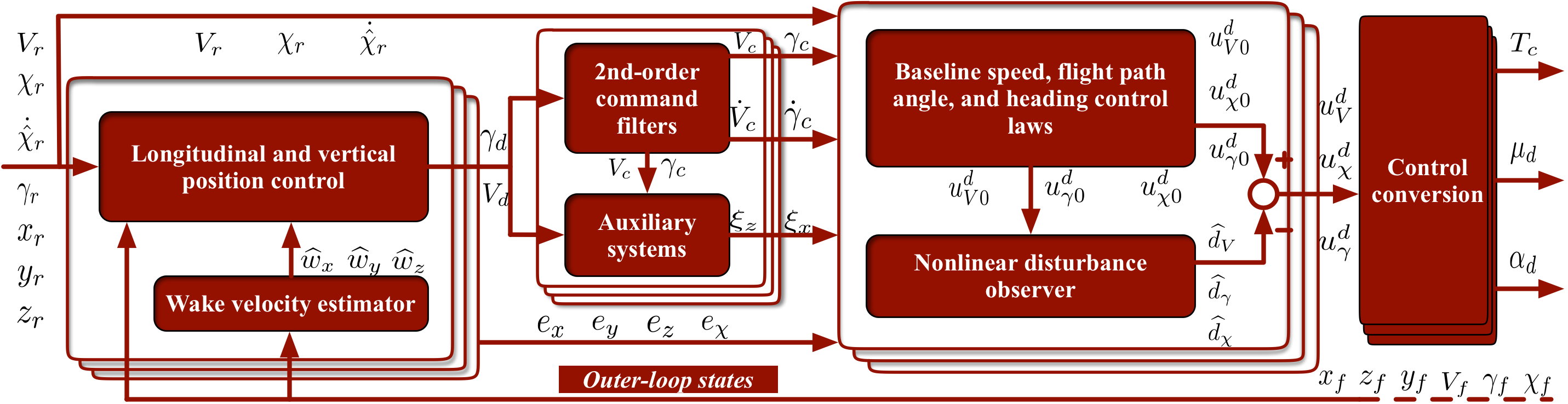
The proposed design in this section can be easily extended to the case with more than three aircraft, even though it is discussed under the leader-follower architecture with two aircraft. In the proposed design, command filtered backstepping technique is employed, which avoids the analytic calculation of time derivatives of intermediate virtual inputs Farrell2005JGCD; Sonneveldt2007JGCD; Farrell2009TAC; Sonneveldt2009JGCD. As shown in Figure 2, the entire design consists of two major loops: an outer loop for formation position control and an inner loop for attitude control. The outer-loop control allows a follower aircraft to track the planned motion by (6), and generates command thrust TcT_{c}, desired bank angle μd\mu_{d}, and desired angle of attack αd\alpha_{d}. The inner-loop control stabilizes follower aircraft’s attitudes to their desired values μd\mu_{d} and αd\alpha_{d} from the outer-loop control, while holding zero sideslip angle βf\beta_{f}.

IV.1 Outer-loop formation position control

Let D¯\overline{D} and L¯\overline{L} be the nominal values of the drag DD and lift LL, respectively. They are obtained by either available aerodynamic data or certain analytical models Morelli1998ACC. The sideslip angle βf\beta_{f} is negligibly small, as it is always stabilized to be zero. Accordingly, the side force YY is small and taken as a model uncertainty. The outer-loop dynamics used for control design are

{x˙f=Vfcosγfcosχf+Wxy˙f=Vfcosγfcosχf+Wyz˙f=−Vfsinγf+Wz{V˙f=1mf(Tcosαfcosβf−D¯)−gsinγf+dVγ˙f=(L¯+Tsinαf)cosμfmf​Vf−gVfcosγf+dγχ˙f=(L¯+Tsinαf)sinμfmfVfcosγf+dχ\left\{\begin{array}[]{lcl}\dot{x}_{f}&=&V_{f}\cos{\gamma_{f}}\cos{\chi_{f}}+W_{x}\\ \dot{y}_{f}&=&V_{f}\cos{\gamma_{f}}\cos{\chi_{f}}+W_{y}\\ \dot{z}_{f}&=&-V_{f}\sin{\gamma_{f}}+W_{z}\end{array}\right.\qquad\left\{\begin{array}[]{lcl}\dot{V}_{f}&=&\frac{1}{m_{f}}\left(T\cos{\alpha_{f}}\cos{\beta_{f}}-\overline{D}\right)-g\sin{\gamma_{f}}+d_{V}\\ \dot{\gamma}_{f}&=&\frac{\left(\overline{L}+T\sin{\alpha_{f}}\right)\cos{\mu_{f}}}{m_{f}V_{f}}-\frac{g}{V_{f}}\cos{\gamma_{f}}+d_{\gamma}\\ \dot{\chi}_{f}&=&\frac{\left(\overline{L}+T\sin{\alpha_{f}}\right)\sin{\mu_{f}}}{m_{f}V_{f}\cos{\gamma_{f}}}+d_{\chi}\end{array}\right. (7)

where xfx_{f}, yf{y}_{f}, and zf{z}_{f} are follower position coordinates in the inertial frame, VfV_{f} is the airspeed, γf\gamma_{f} and χf\chi_{f} are the flight path and heading angles, TT is the thrust, WxW_{x}, WyW_{y}, and WzW_{z} are induced wake velocities, and dVd_{V}, dγd_{\gamma}, and dχd_{\chi} are the augmentation of system uncertainties and disturbances.

{dV=−D−D¯+Δ​Dmf−W˙Wxmfdγ=(L−L¯+ΔL)cosμf−(Y+ΔY−Tcosαfsinβf)sinμfmf​Vf−W˙Wysinμf+W˙Wzcosμfmf​Vfdχ=(L−L¯+ΔL)sinμf+(Y+ΔY−Tcosαfsinβf)cosμfmfVfcosγf+W˙Wycosμf−W˙WzsinμfmfVfcosγf\left\{\begin{array}[]{lcl}d_{V}&=&-\frac{D-\overline{D}+\Delta D}{m_{f}}-\frac{\dot{W}_{W_{x}}}{m_{f}}\\ d_{\gamma}&=&\frac{\left(L-\overline{L}+\Delta L\right)\cos{\mu_{f}}-\left(Y+\Delta Y-T\cos{\alpha_{f}}\sin{\beta_{f}}\right)\sin{\mu_{f}}}{m_{f}V_{f}}-\frac{\dot{W}_{W_{y}}\sin{\mu_{f}}+\dot{W}_{W_{z}}\cos{\mu_{f}}}{m_{f}V_{f}}\\ d_{\chi}&=&\frac{\left(L-\overline{L}+\Delta L\right)\sin{\mu_{f}}+\left(Y+\Delta Y-T\cos{\alpha_{f}}\sin{\beta_{f}}\right)\cos{\mu_{f}}}{m_{f}V_{f}\cos{\gamma_{f}}}+\frac{\dot{W}_{W_{y}}\cos{\mu_{f}}-\dot{W}_{W_{z}}\sin{\mu_{f}}}{m_{f}V_{f}\cos{\gamma_{f}}}\\ \end{array}\right. (8)

where W˙Wx\dot{W}_{W_{x}}, W˙Wy\dot{W}_{W_{y}}, and W˙Wz\dot{W}_{W_{z}} are the wake velocity derivatives denoted in the wind frame of follower aircraft, Δ​L\Delta L, Δ​D\Delta D, and Δ​Y\Delta Y are the vortex-induced forces. According to Zhang2017JA, WxW_{x}, WyW_{y}, and WzW_{z} are bounded, and have much slower dynamics in comparison with aircraft speed and attitudes, so their derivatives are relatively small. Furthermore, the following assumption is introduced.

Assumption 2.

Induced wake velocities WxW_{x}, WyW_{y}, and WzW_{z} are all bounded, and furthermore, they are piecewise constant, namely W˙x=0\dot{W}_{{x}}=0, W˙y=0\dot{W}_{{y}}=0, and W˙z=0\dot{W}_{{z}}=0.

The following nonlinear disturbance observer is employed.

𝐖^=𝝀W+𝓣W−1​𝐗𝐏​, 𝝀˙W=−𝓣−𝟏W​𝝀W−𝓣−𝟏W​(𝓣W−1​𝐗𝐏+𝐔𝐏)\widehat{\mathbf{W}}=\boldsymbol{\lambda}_{W}+\boldsymbol{\mathcal{T}}^{-1}_{W}\mathbf{X_{P}}\text{, }\qquad\boldsymbol{\dot{\lambda}}_{W}=-\boldsymbol{\mathcal{T}^{-1}}_{W}\boldsymbol{\lambda}_{W}-\boldsymbol{\mathcal{T}^{-1}}_{W}\left(\boldsymbol{\mathcal{T}}^{-1}_{W}\mathbf{X_{P}}+\mathbf{{U}_{P}}\right) (9)

where 𝓣W=d​i​a​g​{𝒯W​x​, ​𝒯W​y​, ​𝒯W​z}>0\boldsymbol{\mathcal{T}}_{W}=diag\left\{\mathcal{T}_{Wx}\text{, }\mathcal{T}_{Wy}\text{, }\mathcal{T}_{Wz}\right\}>0, 𝝀W=[λW​x​, ​λW​y​, ​λW​z]T\boldsymbol{\lambda}_{W}=\left[\lambda_{Wx}\text{, }\lambda_{Wy}\text{, }\lambda_{Wz}\right]^{T}, 𝐗𝐏=[xf​, ​yf​, ​zf]T\mathbf{X_{P}}=\left[x_{f}\text{, }y_{f}\text{, }z_{f}\right]^{T}, 𝐔𝐏=[Vfcosγfcosχf, Vfcosγfsinχf, −Vfsinγf]T\mathbf{{U}_{P}}=\left[V_{f}\cos{\gamma_{f}}\cos{\chi_{f}}\text{, }V_{f}\cos{\gamma_{f}}\sin{\chi_{f}}\text{, }-V_{f}\sin{\gamma_{f}}\right]^{T}, 𝐖^=[W^x​, ​W^y​, ​W^z]T\widehat{\mathbf{W}}=\left[\widehat{{W}}_{x}\text{, }\widehat{{W}}_{y}\text{, }\widehat{{W}}_{z}\right]^{T} where W^x\widehat{{W}}_{x}, W^y\widehat{{W}}_{y}, and W^z\widehat{{W}}_{z} are estimates of WxW_{x}, WyW_{y}, and WzW_{z}, respectively. It is chosen that 𝝀W​(0)=−𝓣W−1​𝐗𝐏​(0)\boldsymbol{\lambda}_{W}\left(0\right)=-\boldsymbol{\mathcal{T}}_{W}^{-1}\mathbf{X_{P}}\left(0\right). Let W~x=W^x−Wx\widetilde{W}_{x}=\widehat{W}_{x}-W_{x}, W~y=W^y−Wy\widetilde{W}_{y}=\widehat{W}_{y}-W_{y}, and W~z=W^z−Wz\widetilde{W}_{z}=\widehat{W}_{z}-W_{z}. Under Assumption 2, one has

W~˙x=−W~x/𝒯W​x, W~˙y=−W~y/𝒯W​y,and W~˙z=−W~z/𝒯W​z\dot{\widetilde{W}}_{x}=-\widetilde{W}_{x}/\mathcal{T}_{Wx}\text{, }\qquad\dot{\widetilde{W}}_{y}=-\widetilde{W}_{y}/\mathcal{T}_{Wy}\text{,}\qquad\text{and }\quad\dot{\widetilde{W}}_{z}=-\widetilde{W}_{z}/\mathcal{T}_{Wz} (10)

According to Lemma 1, W~x\widetilde{W}_{x}, W~y\widetilde{W}_{y}, and W~z\widetilde{W}_{z} can be made arbitrarily small by choosing sufficiently small time constants, even if W˙x≠0\dot{W}_{{x}}\neq 0, W˙y≠0\dot{W}_{{y}}\neq 0, and W˙z≠0\dot{W}_{{z}}\neq 0. To simplify the analysis, it is assumed that W~x=W~y=W~z=0\widetilde{W}_{x}=\widetilde{W}_{y}=\widetilde{W}_{z}=0. In light of (9), one has

x˙f=V^fcosγ^fcosχ^f,y˙f=V^fcosγ^fsinχ^f,andz˙f=−V^fsinγ^f\dot{x}_{f}=\widehat{V}_{f}\cos{\widehat{\gamma}_{f}}\cos{\widehat{\chi}_{f}}\text{,}\quad\dot{y}_{f}=\widehat{V}_{f}\cos{\widehat{\gamma}_{f}}\sin{\widehat{\chi}_{f}}\text{,}\quad\text{and}\quad\dot{z}_{f}=-\widehat{V}_{f}\sin{\widehat{\gamma}_{f}} (11)

where

{V^f=(Vfcosγfcosχf+W^x)2+(Vfcosγfcosχf+W^y)2+(−Vfsinγf+W^z)2γ^f=−sin−1⁡(W^z−VfsinγfV^f)χ^f=χf+sin−1⁡(W^ycosχf−W^xsinχfV^fcosγ^f)\small\left\{\begin{array}[]{ll}\widehat{V}_{f}&=\sqrt{\left({V}_{f}\cos{{\gamma}_{f}}\cos{{\chi}_{f}}+\widehat{W}_{x}\right)^{2}+\left({V}_{f}\cos{{\gamma}_{f}}\cos{{\chi}_{f}}+\widehat{W}_{y}\right)^{2}+\left(-{V}_{f}\sin{{\gamma}_{f}}+\widehat{W}_{z}\right)^{2}}\\ \widehat{\gamma}_{f}&=-\sin^{-1}\left(\frac{\widehat{W}_{z}-{V}_{f}\sin{\gamma_{f}}}{\widehat{V}_{f}}\right)\\ \widehat{\chi}_{f}&=\chi_{f}+\sin^{-1}\left(\frac{\widehat{W}_{y}\cos{\chi_{f}}-\widehat{W}_{x}\sin{\chi_{f}}}{\widehat{V}_{f}\cos{\widehat{\gamma}_{f}}}\right)\end{array}\right.

Let xe=xf−xrx_{e}=x_{f}-{x}_{r}, ye=yf−yry_{e}=y_{f}-{y}_{r}, and ze=zf−zrz_{e}=z_{f}-{z}_{r}. Transform xex_{e}, yey_{e}, and zez_{e} into a new frame.

ex=cos⁡χ^f​xe+sin⁡χ^f​ye​, ey=−sin⁡χ^f​xe+cos⁡χ^f​ye​, ez=zee_{x}=\cos{\widehat{\chi}_{f}}x_{e}+\sin{\widehat{\chi}_{f}}y_{e}\text{, }\quad e_{y}=-\sin{\widehat{\chi}_{f}}x_{e}+\cos{\widehat{\chi}_{f}}y_{e}\text{, }\quad e_{z}=z_{e}

We have

{e˙x=V^fcosγ^f−Vrcosγrcoseχ+χ^˙feye˙y=Vrcosγrsineχ−χ^˙fexe˙z=−V^fsinγ^f+Vrsinγr\left\{\begin{array}[]{lcl}\dot{e}_{x}&=&\widehat{V}_{f}\cos{\widehat{\gamma}_{f}}-{V}_{r}\cos{{\gamma}_{r}}\cos{e_{\chi}}+\dot{\widehat{\chi}}_{f}e_{y}\\ \dot{e}_{y}&=&{V}_{r}\cos{{\gamma}_{r}}\sin{e_{\chi}}-\dot{\widehat{\chi}}_{f}e_{x}\\ \dot{e}_{z}&=&-\widehat{V}_{f}\sin{\widehat{\gamma}_{f}}+{V}_{r}\sin{{\gamma}_{r}}\end{array}\right. (12)

where eχ=χ^f−χre_{\chi}=\widehat{\chi}_{f}-\chi_{r}. The desired velocity and flight path angle are shown in (13).

Vd=(−Kxex+Vrcosγrcoseχ)/cosγ^f−δV, γd=sin−1((Kzez+Vrsinγr+W^z)/Vf)V_{d}=\left(-K_{x}e_{x}+V_{r}\cos\gamma_{r}\cos{e_{\chi}}\right)/\cos{\widehat{\gamma}_{f}}-\delta V\text{, }\quad\gamma_{d}=\sin^{-1}\left(\left({K_{z}e_{z}+V_{r}\sin\gamma_{r}+\widehat{W}_{z}}\right)/{V_{f}}\right) (13)

where Kx​, ​Kz>0K_{x}\text{, }K_{z}>0 are control parameters, and δ​V=V^f−Vf\delta V=\widehat{V}_{f}-V_{f}. The desired signals VdV_{d} and γd\gamma_{d} are passed through a command filter to obtain VcV_{c}, γc\gamma_{c}, and their rates. Hence,

[𝒮˙c𝒮¨c]=[0​,1−ω𝒮2​,−2​ζ𝒮​ω𝒮]​[𝒮c𝒮˙c]+[0ω𝒮2]​𝒮d​, 𝒮∈{V​, ​γ}\left[\begin{array}[]{c}\dot{\mathscr{S}}_{c}\\ \ddot{\mathscr{S}}_{c}\end{array}\right]=\left[\begin{array}[]{cc}0\text{,}&1\\ -\omega_{\mathscr{S}}^{2}\text{,}&-2\zeta_{\mathscr{S}}\omega_{\mathscr{S}}\end{array}\right]\left[\begin{array}[]{c}\mathscr{S}_{c}\\ \dot{\mathscr{S}}_{c}\end{array}\right]+\left[\begin{array}[]{c}0\\ \omega_{\mathscr{S}}^{2}\end{array}\right]\mathscr{S}_{d}\text{, }\quad\mathscr{S}\in\left\{V\text{, }\gamma\right\} (14)

Let eV=Vf−Vce_{V}=V_{f}-V_{c} and eγ=γf−γce_{\gamma}=\gamma_{f}-\gamma_{c}. Note that L¯=L¯0+L¯α​αf\overline{L}=\overline{L}_{0}+\overline{L}_{\alpha}\alpha_{f} where L¯0\overline{L}_{0} is the lift at αf=0\alpha_{f}=0 and L¯α\overline{L}_{\alpha} is the lift derivative with respect to the angle of attack. According to (7), one has

{e˙V=Tcosαfcosβf−D¯mf−gsinγf⏟uV−V˙c+dVe˙γ=(L¯0+L¯ααf+Tsinαf)cosμf−mfgcosγfmf​Vf⏟uγ−γ˙c+dγe˙χ=(L¯0+L¯ααf+Tsinαf)sinμfmfVfcosγf⏟uχ−χ^˙r+dχ\left\{\begin{array}[]{lcl}\dot{e}_{V}&=&\underbrace{\frac{T\cos{\alpha_{f}}\cos{\beta_{f}}-\overline{D}}{m_{f}}-g\sin{\gamma_{f}}}_{u_{V}}-\dot{V}_{c}+d_{V}\\ \dot{e}_{\gamma}&=&\underbrace{\frac{\left(\overline{L}_{0}+\overline{L}_{\alpha}\alpha_{f}+T\sin{\alpha_{f}}\right)\cos{\mu_{f}}-m_{f}g\cos{\gamma_{f}}}{m_{f}V_{f}}}_{u_{\gamma}}-\dot{\gamma}_{c}+d_{\gamma}\\ \dot{e}_{\chi}&=&\underbrace{\frac{\left(\overline{L}_{0}+\overline{L}_{\alpha}\alpha_{f}+T\sin{\alpha_{f}}\right)\sin{\mu_{f}}}{m_{f}V_{f}\cos{\gamma_{f}}}}_{u_{\chi}}-\dot{\widehat{\chi}}_{r}+{d}_{\chi}\end{array}\right. (15)

where uVu_{V}, uγu_{\gamma}, and uχu_{\chi} are intermediate control inputs, χ^˙r\dot{\widehat{\chi}}_{r} is the estimation of χ˙r\dot{\chi}_{r} by passing χr\chi_{r} through a 2nd-order filter similar to (5). Two more uncertainty terms χ~˙r{\dot{\widetilde{\chi}}}_{r} and χ~˙f\dot{\widetilde{\chi}}_{f} are included in dχ{d}_{\chi} in (15), where χ~˙r=χ^˙r−χ˙r{\dot{\widetilde{\chi}}}_{r}={\dot{\widehat{\chi}}}_{r}-\dot{\chi}_{r} and χ~˙f=dd​t​sin−1⁡(W^ycosχf−W^xsinχfV^fcosγ^f)\dot{\widetilde{\chi}}_{f}=\frac{d}{dt}\sin^{-1}\left(\frac{{\widehat{W}}_{y}\cos{\chi_{f}}-\widehat{W}_{x}\sin{\chi_{f}}}{\widehat{V}_{f}\cos{\widehat{\gamma}_{f}}}\right). Hence, dχ{d}_{\chi} in (15) is re-defined to be dχ=(L−L¯+ΔL)sinμf+(Y+ΔY−cosαfsinβf)cosμfmfVfcosγf+χ~˙r+χ~˙f+W˙Wycosμf−W˙WzsinμfmfVfcosγf{d}_{\chi}=\frac{\left(L-\overline{L}+\Delta L\right)\sin{\mu_{f}}+\left(Y+\Delta Y-\cos{\alpha_{f}}\sin{\beta_{f}}\right)\cos{\mu_{f}}}{m_{f}V_{f}\cos{\gamma_{f}}}+\dot{\widetilde{\chi}}_{r}+\dot{\widetilde{\chi}}_{f}+\frac{\dot{W}_{W_{y}}\cos{\mu_{f}}-\dot{W}_{W_{z}}\sin{\mu_{f}}}{m_{f}V_{f}\cos{\gamma_{f}}}. Note that χr\chi_{r} is a smooth signal with bounded derivatives. According to Lemma 2, χ~˙r{\dot{\widetilde{\chi}}}_{r} and its derivative are bounded, so χ~˙f{\dot{\widetilde{\chi}}}_{f} and its derivative are also bounded.

Assumption 3.

The uncertainties and disturbances dVd_{V}, dγd_{\gamma}, dχd_{\chi}, and their derivatives are bounded.

The following virtual inputs uVdu_{V}^{d}, uγdu_{\gamma}^{d}, and uχdu_{\chi}^{d} are choosing for the error systems (12) and (15).

uVd=uV​0d−d^V+V˙c​,uγd=uγ​0d−d^γ+γ˙c​,anduχd=uχ​0d−d^χ+χ^˙ru_{V}^{d}=u_{V0}^{d}-\widehat{d}_{V}+\dot{V}_{c}\text{,}\quad u_{\gamma}^{d}=u_{\gamma 0}^{d}-\widehat{d}_{\gamma}+\dot{\gamma}_{c}\text{,}\quad\text{and}\quad u_{\chi}^{d}=u_{\chi 0}^{d}-\widehat{d}_{\chi}+\dot{\widehat{\chi}}_{r}\vskip-8.53581pt (16)

where d^V\widehat{d}_{V}, d^γ\widehat{d}_{\gamma}, and d^χ\widehat{{d}}_{\chi} are estimates of dV{d}_{V}, dγ{d}_{\gamma}, and dχ{{d}}_{\chi}, respectively, and uV​0du_{V0}^{d}, uγ​0du_{\gamma 0}^{d}, and uχ​0du_{\chi 0}^{d} are

uV​0d=−KV​eV−cVεxcosγ^fH​,uγ​0d=−Kγ​eγ​,anduχ​0d=−Kχ​eχ−cχeyVrcosγrcos(eχ2)H{u}_{V0}^{d}=-K_{V}e_{V}-\frac{c_{V}\varepsilon_{x}\cos\widehat{\gamma}_{f}}{H}\text{,}\quad u_{\gamma 0}^{d}=-K_{\gamma}e_{\gamma}\text{,}\quad\text{and}\quad u_{\chi 0}^{d}=-K_{\chi}e_{\chi}-\frac{c_{\chi}e_{y}V_{r}\cos{\gamma_{r}}\cos\left(\frac{e_{\chi}}{2}\right)}{H} (17)

where KVK_{V}, KγK_{\gamma}, KχK_{\chi}, cVc_{V}, cχ>0c_{\chi}>0 are control parameters, H=εx2+ey2+1H=\sqrt{\varepsilon_{x}^{2}+e_{y}^{2}+1}, εx=ex−ξx\varepsilon_{x}=e_{x}-\xi_{x}, and εz=ez−ξz\varepsilon_{z}=e_{z}-\xi_{z}, where ξx\xi_{x} and ξz\xi_{z} in (18) are used to counteract the estimation errors in the filter (14).

ξ˙x=−Kxξx+(Vc−Vd)cosγ^f,ξ˙z=−Kzξz+Vf(sinγd−sinγf)\dot{\xi}_{x}=-K_{x}\xi_{x}+\left(V_{c}-V_{d}\right)\cos\widehat{\gamma}_{f}\text{,}\qquad\dot{\xi}_{z}=-K_{z}\xi_{z}+V_{f}\left(\sin\gamma_{d}-\sin\gamma_{f}\right)\vskip-8.53581pt (18)
Refer to caption
Figure 3: Command filter and auxiliary system for speed control

Shown in Figure 3 is the command filter and auxiliary system for speed control. If one chooses uV=uVdu_{V}={u}_{V}^{d}, uγ=uγdu_{\gamma}={u}_{\gamma}^{d}, and uχ=uχdu_{\chi}={u}_{\chi}^{d}, there exists

{V˙f=−KV​eV−cV​εxcosγ^fH+V˙c−d^V+dVγ˙f=−Kγ​eγ+γ˙c−d^γ+dγχ˙f=−Kχ​sin⁡(eχ2)−cχeyVrcosγrcos(eχ2)H+χ^˙r−d^χ+dχ\left\{\begin{array}[]{lcl}\dot{V}_{f}&=&-K_{V}e_{V}-c_{V}\frac{\varepsilon_{x}\cos\widehat{\gamma}_{f}}{H}+\dot{V}_{c}-\widehat{d}_{V}+d_{V}\\ \dot{\gamma}_{f}&=&-K_{\gamma}e_{\gamma}+\dot{\gamma}_{c}-\widehat{d}_{\gamma}+d_{\gamma}\\ \dot{\chi}_{f}&=&-K_{\chi}\sin\left(\frac{e_{\chi}}{2}\right)-\frac{c_{\chi}e_{y}V_{r}\cos{\gamma_{r}}\cos\left(\frac{e_{\chi}}{2}\right)}{H}+\dot{\widehat{\chi}}_{r}-\widehat{{d}}_{\chi}+{d}_{\chi}\end{array}\right. (19)

Based on (19), the nonlinear disturbance observer is

𝐃^𝐃=𝝀𝑫+𝓣𝑫−𝟏​𝐗𝐃​, 𝝀˙𝑫=−𝓣𝑫−𝟏​𝝀𝑫−𝓣𝑫−𝟏​(𝓣𝑫−𝟏​𝐗𝐃+𝐔𝐃−𝐃^𝐃)\mathbf{\widehat{D}_{D}}=\boldsymbol{\lambda_{D}}+\boldsymbol{\mathcal{T}_{D}^{-1}}\mathbf{X_{D}}\text{, }\qquad\boldsymbol{\dot{\lambda}_{D}}=-\boldsymbol{\mathcal{T}_{D}^{-1}}\boldsymbol{\lambda_{D}}-\boldsymbol{\mathcal{T}_{D}^{-1}}\left(\boldsymbol{\mathcal{T}_{D}^{-1}}\mathbf{X_{D}}+\mathbf{U_{D}}-\mathbf{\widehat{D}_{D}}\right) (20)

where 𝓣𝑫=d​i​a​g​{𝒯V​, ​𝒯γ​, ​𝒯χ}>0\boldsymbol{\mathcal{T}_{D}}=diag\left\{\mathcal{T}_{V}\text{, }\mathcal{T}_{\gamma}\text{, }\mathcal{T}_{\chi}\right\}>0 is a positive definite constant matrix, 𝝀𝑫=[λV​, ​λγ​, ​λχ]T\boldsymbol{\lambda_{D}}=\left[\lambda_{V}\text{, }\lambda_{\gamma}\text{, }\lambda_{\chi}\right]^{T}, 𝐗𝐃=[Vf​, ​γf​, ​χf]T\mathbf{X_{D}}=\left[V_{f}\text{, }\gamma_{f}\text{, }\chi_{f}\right]^{T}, 𝐔𝐃=[uV​0d​, ​uγ​0d​, ​uχ​0d]T\mathbf{U_{D}}=\left[{u}_{V0}^{d}\text{, }u_{\gamma 0}^{d}\text{, }u_{\chi 0}^{d}\right]^{T}, and 𝐃^𝐃=[d^V​, ​d^γ​, ​d^χ]T\mathbf{\widehat{D}_{D}}=\left[\widehat{d}_{V}\text{, }\widehat{d}_{\gamma}\text{, }\widehat{d}_{\chi}\right]^{T}. The uncertainty and disturbance estimates d^V\widehat{d}_{V}, d^γ\widehat{d}_{\gamma}, and d^χ\widehat{{d}}_{\chi} need to be fed back to the estimator for the next estimation updates. Combining (17) and (20), one is able to get uVdu_{V}^{d}, uγdu_{\gamma}^{d}, and uχdu_{\chi}^{d}. Hence,

{Tc=mf(uVd+gsinγf)+D¯cosαfcosβfαd=mfVf(uγd+gVcosγf)2+(uχd)2cos2γf−Tsinαf−L¯0L¯αμd=tan−1⁡(mfVfuχdcosγfmfVfuγ+mfgcosγf)\left\{\begin{array}[]{lcl}T_{c}&=&\frac{m_{f}\left(u_{V}^{d}+g\sin{\gamma_{f}}\right)+\overline{D}}{\cos{\alpha_{f}}\cos{\beta_{f}}}\\ \alpha_{d}&=&\frac{m_{f}V_{f}\sqrt{\left(u_{\gamma}^{d}+\frac{g}{V}\cos{\gamma_{f}}\right)^{2}+\left(u_{\chi}^{d}\right)^{2}\cos^{2}{\gamma_{f}}}-T\sin{\alpha_{f}}-\overline{L}_{0}}{\overline{L}_{\alpha}}\\ \mu_{d}&=&\tan^{-1}\left(\frac{m_{f}V_{f}u_{\chi}^{d}\cos{\gamma_{f}}}{m_{f}V_{f}u_{\gamma}+m_{f}g\cos{\gamma_{f}}}\right)\end{array}\right. (21)
Refer to caption
Figure 4: The outer-loop formation position control structure

The entire outer-loop control structure is illustrated in Figure 4. The following assumption is introduced for dV{d_{V}}, dγ{d_{\gamma}}, and dχ{d_{\chi}} for the stability analysis.

Assumption 4.

dV{d_{V}}, dγ{d_{\gamma}}, and dχ{d_{\chi}} have slow dynamics, and furthermore, d˙V≃0\dot{d}_{V}\simeq 0, d˙γ≃0\dot{d}_{\gamma}\simeq 0, and d˙χ≃0\dot{d}_{\chi}\simeq 0.

The following error dynamics will be obtained.

{ε˙x=V^fcosγ^f−Vrcosγrcoseχ−ξ˙x+χ^˙feye˙y=Vrcosγrsineχ−χ^˙fεxε˙z=−V^fsinγ^f+Vrsinγr−ξ˙z\left\{\begin{array}[]{lcl}\dot{\varepsilon}_{x}&=&\widehat{V}_{f}\cos{\widehat{\gamma}_{f}}-{V}_{r}\cos{{\gamma}_{r}}\cos{e_{\chi}}-\dot{\xi}_{x}+\dot{\widehat{\chi}}_{f}e_{y}\\ \dot{e}_{y}&=&{V}_{r}\cos{{\gamma}_{r}}\sin{e_{\chi}}-\dot{\widehat{\chi}}_{f}\varepsilon_{x}\\ \dot{\varepsilon}_{z}&=&-\widehat{V}_{f}\sin{\widehat{\gamma}_{f}}+{V}_{r}\sin{{\gamma}_{r}}-\dot{\xi}_{z}\end{array}\right. (22)

Assume αf\alpha_{f} and μf\mu_{f} are able to be rapidly stabilized by its inner-loop attitude controller to their desired values αd\alpha_{d} and μd\mu_{d}, respectively. The following theorem holds.

Theorem 1.

If Assumptions 3 and 4 hold, and KVK_{V}, KγK_{\gamma}, KχK_{\chi}, 𝒯V\mathcal{T}_{V}, 𝒯γ\mathcal{T}_{\gamma}, 𝒯χ\mathcal{T}_{\chi}, cVc_{V}, cχ>0c_{\chi}>0, 0<Kx<2​ζV​ωV0<K_{x}<2\zeta_{V}\omega_{V}, and 0<Kz<2​ζγ​ωγ0<K_{z}<2\zeta_{\gamma}\omega_{\gamma}, the proposed outer-loop formation controller given by (16), (17), and (20) will stabilize the outer-loop formation error system composed of (15) and (22), and

limt→∞ex→ξx​, limt→∞ez→ξz​,  and limt→∞ey→0\lim_{t\to\infty}e_{x}\to\xi_{x}\text{, }\quad\lim_{t\to\infty}e_{z}\to\xi_{z}\text{, }\quad\text{ and }\quad\lim_{t\to\infty}e_{y}\to 0\vskip-8.53581pt

where ξx\xi_{x} and ξz\xi_{z} will be ultimately arbitrarily bounded by control parameters ωV\omega_{V}, KxK_{x}, and ωγ\omega_{\gamma}, KzK_{z}, respectively. If ξx​(0)=ξz​(0)=0\xi_{x}\left(0\right)=\xi_{z}\left(0\right)=0, there exist

limt→∞ξx≤1Kx∥Vc−Vd∥∞ and limt→∞ξx≤1Kz∥Vf∥∞∥sinγd−sinγf∥∞\lim_{t\to\infty}{\xi}_{x}\leq\frac{1}{K_{x}}\|V_{c}-V_{d}\|_{\infty}\text{ }\quad\text{and }\quad\lim_{t\to\infty}{\xi}_{x}\leq\frac{1}{K_{z}}\|V_{f}\|_{\infty}\|\sin{\gamma_{d}}-\sin{\gamma_{f}}\|_{\infty}\vskip-8.53581pt (23)

where Vc−VdV_{c}-V_{d} will exponentially converge to 𝒪⁡(1ωV)\mathcal{O}\left(\frac{1}{\omega_{V}}\right) and limt→∞γf−γd→𝒪⁡(1ωγ)\lim_{t\to\infty}\gamma_{f}-\gamma_{d}\to\mathcal{O}\left(\frac{1}{\omega_{\gamma}}\right). Therefore, by tuning ωV\omega_{V}, KxK_{x}, and ωγ\omega_{\gamma}, KzK_{z}, the ultimate boundaries of ex{e}_{x} and ez{e}_{z} could be regulated accordingly.

Proof.

Let d~i=d^i−di\widetilde{d}_{i}=\widehat{d}_{i}-d_{i} (i∈{V​, ​γ​, ​χ}i\in\left\{V\text{, }\gamma\text{, }\chi\right\}). If Assumption 4 holds, and αf\alpha_{f} and μf\mu_{f} are rapidly stabilized to be αd\alpha_{d} and μd\mu_{d}, respectively, it is easily to obtain

d~V˙=−d~V𝒯V​,d~γ˙=−d~γ𝒯γ​,andd~V˙=−d~χ𝒯χ\dot{\widetilde{{d}}_{V}}=-\frac{\widetilde{d}_{V}}{\mathcal{T}_{V}}\text{,}\quad\dot{\widetilde{{d}}_{\gamma}}=-\frac{\widetilde{d}_{\gamma}}{\mathcal{T}_{\gamma}}\text{,}\quad\text{and}\quad\dot{\widetilde{{d}}_{V}}=-\frac{\widetilde{d}_{\chi}}{\mathcal{T}_{\chi}}\vskip-8.53581pt (24)

Based on (15), (22), and (24), Theorem 1 is proven in two steps. The first step shows limt→∞εx→0\lim_{t\to\infty}\varepsilon_{x}\to 0, limt→∞ey→0\lim_{t\to\infty}e_{y}\to 0, and limt→∞εz→0\lim_{t\to\infty}\varepsilon_{z}\to 0, and thus limt→∞ex→ξx\lim_{t\to\infty}e_{x}\to\xi_{x} and limt→∞ez→ξz\lim_{t\to\infty}e_{z}\to\xi_{z}. The second step demonstrates that ξx\xi_{x} and ξz\xi_{z} are uniformly ultimately bounded, which implies exe_{x} and eze_{z} are ultimately bounded. The ultimate boundaries of exe_{x} and eze_{z} are related to control gains.

To show limt→∞εx→0\lim_{t\to\infty}\varepsilon_{x}\to 0, limt→∞ey→0\lim_{t\to\infty}e_{y}\to 0, and limt→∞εz→0\lim_{t\to\infty}\varepsilon_{z}\to 0, we choose

𝕍=H+εz22+8​cχ−1​sin2⁡(eχ4)+cV−1​eV22+eγ22+cχ−1​d~χ22+cV−1​d~V22+d~γ22−1\mathbb{V}=H+\frac{\varepsilon_{z}^{2}}{2}+8c_{\chi}^{-1}\sin^{2}{\left(\frac{e_{\chi}}{4}\right)}+c_{V}^{-1}\frac{e_{V}^{2}}{2}+\frac{e_{\gamma}^{2}}{2}+c_{\chi}^{-1}\frac{\widetilde{d}_{\chi}^{2}}{2}+c_{V}^{-1}\frac{{\widetilde{d}_{V}}^{2}}{2}+\frac{\widetilde{d}_{\gamma}^{2}}{2}-1

where H=εx2+ey2+1H=\sqrt{\varepsilon_{x}^{2}+e_{y}^{2}+1}. Differentiating 𝕍\mathbb{V} yields

𝕍˙1\displaystyle\dot{\mathbb{V}}_{1} =\displaystyle= εx​ε˙xH+ey​e˙yH+εz​ε˙z+2​cχ−1​sin⁡(eχ2)​e˙χ+cV−1​eV​e˙V+eγ​e˙γ+cχ−1​d~χ​d~χ˙+d~γ​d~γ˙+cV−1​d~V​d~V˙\displaystyle\frac{\varepsilon_{x}\dot{\varepsilon}_{x}}{H}+\frac{e_{y}\dot{e}_{y}}{H}+\varepsilon_{z}\dot{\varepsilon}_{z}+2c_{\chi}^{-1}\sin{\left(\frac{e_{\chi}}{2}\right)}\dot{e}_{\chi}+c_{V}^{-1}{e_{V}}{\dot{e}_{V}}+{e_{\gamma}}\dot{e}_{\gamma}+c_{\chi}^{-1}\widetilde{d}_{\chi}\dot{\widetilde{d}_{\chi}}+\widetilde{d}_{\gamma}\dot{\widetilde{d}_{\gamma}}+c_{V}^{-1}\widetilde{d}_{V}\dot{\widetilde{d}_{V}} (25)
=\displaystyle= −Kx​εx2H+cV−1​eV​(uV−V˙c+dV+cVεxcosγ^fH)−Kz​εz2+eγ​(uγ−γ˙c+dγ)\displaystyle-K_{x}\frac{\varepsilon_{x}^{2}}{H}+c_{V}^{-1}{e_{V}}\left({u_{V}}-\dot{V}_{c}+d_{V}+\frac{{c_{V}}{\varepsilon_{x}\cos{\widehat{\gamma}_{f}}}}{H}\right)-K_{z}\varepsilon_{z}^{2}+{e_{\gamma}}\left({u_{\gamma}}-\dot{\gamma}_{c}+d_{\gamma}\right)
+2​cχ−1​sin⁡(eχ2)​(uχ−χ^˙r+dχ+cχeyVrcosγrcoseχ2H)−cχ−1​d~χ2𝒯χ−cV−1​d~V2𝒯V−d~γ2𝒯γ\displaystyle+2c_{\chi}^{-1}\sin{\left(\frac{e_{\chi}}{2}\right)}\left({u_{\chi}}-\dot{\widehat{\chi}}_{r}+d_{\chi}+\frac{{c_{\chi}}e_{y}{V}_{r}\cos{{\gamma}_{r}}\cos{\frac{e_{\chi}}{2}}}{H}\right)-c_{\chi}^{-1}\frac{\widetilde{d}_{\chi}^{2}}{\mathcal{T}_{\chi}}-c_{V}^{-1}\frac{{\widetilde{d}_{V}}^{2}}{\mathcal{T}_{V}}-\frac{\widetilde{d}_{\gamma}^{2}}{\mathcal{T}_{\gamma}}

Substituting (16) and (17) for corresponding terms in (25) yields

𝕍˙1=−cχ−1​[sin⁡(eχ2)​, ​d~χ]​[2​Kχ−1−11𝒯χ]​[sin⁡(eχ2)d~χ]−cV−1​[eV​, ​d~V]​[KV−0.5−0.51𝒯V]​[eVd~V]−[eγ​, ​d~γ]​[Kγ−0.5−0.51𝒯γ]​[eγd~γ]−Kx​εx2H−Kz​εz2\small\begin{array}[]{ll}\dot{\mathbb{V}}_{1}&=-c_{\chi}^{-1}\left[\sin{\left(\frac{e_{\chi}}{2}\right)}\text{, }\widetilde{d}_{\chi}\right]\left[\begin{array}[]{cc}2K_{\chi}&-1\\ -1&\frac{1}{\mathcal{T}_{\chi}}\end{array}\right]\left[\begin{array}[]{c}\sin{\left(\frac{e_{\chi}}{2}\right)}\\ \widetilde{d}_{\chi}\end{array}\right]-c_{V}^{-1}\left[e_{V}\text{, }\widetilde{d}_{V}\right]\left[\begin{array}[]{cc}K_{V}&-0.5\\ -0.5&\frac{1}{\mathcal{T}_{V}}\end{array}\right]\left[\begin{array}[]{c}e_{V}\\ \widetilde{d}_{V}\end{array}\right]\\ &-\left[e_{\gamma}\text{, }\widetilde{d}_{\gamma}\right]\left[\begin{array}[]{cc}K_{\gamma}&-0.5\\ -0.5&\frac{1}{\mathcal{T}_{\gamma}}\end{array}\right]\left[\begin{array}[]{c}e_{\gamma}\\ \widetilde{d}_{\gamma}\end{array}\right]-K_{x}\frac{\varepsilon_{x}^{2}}{H}-K_{z}\varepsilon_{z}^{2}\end{array}

If KV​, ​Kχ​, ​Kγ​, ​𝒯V​, ​𝒯γ​, ​𝒯χ>0K_{V}\text{, }K_{\chi}\text{, }K_{\gamma}\text{, }\mathcal{T}_{V}\text{, }\mathcal{T}_{\gamma}\text{, }\mathcal{T}_{\chi}>0, one has

[2​Kχ−1−11𝒯χ]>0​,[KV−0.5−0.51𝒯V]>0​,and[Kγ−0.5−0.51𝒯γ]>0\small\left[\begin{array}[]{cc}2K_{\chi}&-1\\ -1&\frac{1}{\mathcal{T}_{\chi}}\end{array}\right]>0\text{,}\hskip 18.49988pt\left[\begin{array}[]{cc}K_{V}&-0.5\\ -0.5&\frac{1}{\mathcal{T}_{V}}\end{array}\right]>0\text{,}\hskip 18.49988pt\text{and}\hskip 18.49988pt\left[\begin{array}[]{cc}K_{\gamma}&-0.5\\ -0.5&\frac{1}{\mathcal{T}_{\gamma}}\end{array}\right]>0

Hence, there exists 𝕍˙1≤0\dot{\mathbb{V}}_{1}\leq 0 by choosing Kx>0K_{x}>0, Kz>0K_{z}>0, cV>0c_{V}>0, and cχ>0c_{\chi}>0. Therefore, 𝕍\mathbb{V} is a non-increasing positive definite function, which implies 𝕍⁡(∞)≤𝕍⁡(0)\mathbb{V}(\infty)\leq\mathbb{V}(0) is a finite constant and limt→∞∫0t𝕍˙1​(τ)​𝑑τ=𝕍⁡(∞)−𝕍⁡(0)\lim_{t\to\infty}\int^{t}_{0}\dot{\mathbb{V}}_{1}(\tau)d\tau=\mathbb{V}(\infty)-\mathbb{V}(0) exists and is finite. Thus, 𝕍\mathbb{V} is bounded and has a finite limit as t→∞t\to\infty, and εx\varepsilon_{x}, eye_{y}, εz\varepsilon_{z}, eχe_{\chi}, eVe_{V}, eγe_{\gamma}, d~V\widetilde{d}_{V}, d~χ\widetilde{d}_{\chi}, and d~γ\widetilde{d}_{\gamma} are all bounded as well. Furthermore, 𝕍¨1\ddot{\mathbb{V}}_{1} is also bounded, as it is a function of εx\varepsilon_{x}, eye_{y}, εz\varepsilon_{z}, eχe_{\chi}, eVe_{V}, eγe_{\gamma}, d~V\widetilde{d}_{V}, d~χ\widetilde{d}_{\chi}, and d~γ\widetilde{d}_{\gamma}. Hence, 𝕍˙1\dot{\mathbb{V}}_{1} is uniformly continuous. According to Barbǎlat’s lemma Ioannou1995Book, limt→∞𝕍˙1→0\lim_{t\to\infty}\dot{\mathbb{V}}_{1}\to 0, so limt→∞εx→0​, ​εz→0​, ​limt→∞eχ→0​, ​limt→∞eV→0​, ​limt→∞eγ→0\lim_{t\to\infty}\varepsilon_{x}\to 0\text{, }\varepsilon_{z}\to 0\text{, }\lim_{t\to\infty}e_{\chi}\to 0\text{, }\lim_{t\to\infty}e_{V}\to 0\text{, }\lim_{t\to\infty}e_{\gamma}\to 0, limt→∞d~V→0\lim_{t\to\infty}\widetilde{d}_{V}\to 0, limt→∞d~χ→0\lim_{t\to\infty}\widetilde{d}_{\chi}\to 0, limt→∞d~γ→0\lim_{t\to\infty}\widetilde{d}_{\gamma}\to 0. It is obviously that limt→∞ex→ξx\lim_{t\to\infty}e_{x}\to\xi_{x} and limt→∞ez→ξz\lim_{t\to\infty}e_{z}\to\xi_{z}. One could apply Barbǎlat’s lemma to e˙χ\dot{e}_{\chi} to show limt→∞ey→0\lim_{t\to\infty}e_{y}\to 0. Differentiating e˙χ\dot{e}_{\chi} by time will yield

e¨χ\displaystyle\ddot{e}_{\chi} =\displaystyle= −Kψe˙χ2coseχ2−cχH˙eyVrcosγrcoseχ2H2+cχHe˙yVrcosγrcoseχ2+cχHeyV˙rcosγrcoseχ2\displaystyle-K_{\psi}\frac{\dot{e}_{\chi}}{2}\cos{\frac{e_{\chi}}{2}}-\frac{c_{\chi}\dot{H}e_{y}V_{r}\cos{\gamma_{r}}\cos{\frac{e_{\chi}}{2}}}{H^{2}}+\frac{c_{\chi}}{H}\dot{e}_{y}V_{r}\cos{\gamma_{r}}\cos{\frac{e_{\chi}}{2}}+\frac{c_{\chi}}{H}e_{y}\dot{V}_{r}\cos{\gamma_{r}}\cos{\frac{e_{\chi}}{2}}
−cχHγ˙reyVrsinγrcoseχ2−cχHe˙χ2eyVrcosγrsineχ2−d~χ𝒯χ\displaystyle-\frac{c_{\chi}}{H}\dot{\gamma}_{r}{e}_{y}V_{r}\sin{\gamma_{r}}\cos{\frac{e_{\chi}}{2}}-\frac{c_{\chi}}{H}\frac{\dot{e}_{\chi}}{2}{e}_{y}V_{r}\cos{\gamma_{r}}\sin{\frac{e_{\chi}}{2}}-\frac{\widetilde{d}_{\chi}}{\mathcal{T}_{\chi}}

Obviously, χ¨e\ddot{\chi}_{e} is bounded according to Lemma 1 and Assumptions 1 and 3. Considering ∫e˙χ​𝑑t=eχ\int\dot{e}_{\chi}dt=e_{\chi} and limt→∞eχ→0\lim_{t\to\infty}e_{\chi}\to 0, we have ψ˙e→0\dot{\psi}_{e}\to 0 as t→∞t\to\infty in accordance with Barbǎlat’s lemma. According to (15), (16), and (17), ey=−e˙χ+Kχ​eχ+d~χcχVrcosγrcoseχ2​He_{y}=-\frac{\dot{e}_{\chi}+K_{\chi}e_{\chi}+\widetilde{d}_{\chi}}{c_{\chi}V_{r}\cos{\gamma_{r}}\cos{\frac{e_{\chi}}{2}}}H. Since limt→∞e˙χ→0\lim_{t\to\infty}\dot{e}_{\chi}\to 0, limt→∞eχ→0\lim_{t\to\infty}e_{\chi}\to 0, limt→∞d~χ→0\lim_{t\to\infty}\widetilde{d}_{\chi}\to 0, cχVrcosγrcoseχ2>0c_{\chi}V_{r}\cos{\gamma_{r}}\cos{\frac{e_{\chi}}{2}}>0, and H>0H>0, it is readily to conclude that limt→∞ey→0\lim_{t\to\infty}e_{y}\to 0.

The second step shows that ξx\xi_{x} and ξz\xi_{z} are uniformly ultimately bounded. From (13), one has

Vd=(−Kxex+Vrcosγr)/cosγ^f−δV=(−Kxεx−Kxξx+Vrcosγrcoseχ)/cosγ^f−δVV_{d}={\left(-K_{x}e_{x}+V_{r}\cos\gamma_{r}\ \right)}/{\cos{\widehat{\gamma}_{f}}}-\delta V={\left(-K_{x}\varepsilon_{x}-K_{x}\xi_{x}+V_{r}\cos\gamma_{r}\cos{e_{\chi}}\right)}/{\cos{\widehat{\gamma}_{f}}}-\delta V (26)

Substituting the equation above for VdV_{d} in (14) and (18) will generate

[ξ˙xV˙cV¨c]=[0cos⁡γ^f0001−Kx​ωV2cos⁡γ^f−ωV2−2​ζV​ωV]⏟𝐀v​[ξxVcV˙c]−[cos⁡γ^f0ωV2]​(Vrcosγrcoseχ−Kxεxcos⁡γ^f+δ​V)\left[\begin{array}[]{c}\dot{\xi}_{x}\\ \dot{V}_{c}\\ \ddot{V}_{c}\end{array}\right]=\underbrace{\left[\begin{array}[]{ccc}0&\cos{\widehat{\gamma}_{f}}&0\\ 0&0&1\\ -\frac{K_{x}\omega_{V}^{2}}{\cos{\widehat{\gamma}_{f}}}&-\omega_{V}^{2}&-2\zeta_{V}\omega_{V}\end{array}\right]}_{\mathbf{A}_{v}}\left[\begin{array}[]{c}{\xi}_{x}\\ {V}_{c}\\ \dot{V}_{c}\end{array}\right]-\left[\begin{array}[]{c}\cos{\widehat{\gamma}_{f}}\\ 0\\ \omega_{V}^{2}\end{array}\right]\left(\frac{V_{r}\cos{\gamma_{r}}\cos{e_{\chi}}-K_{x}\varepsilon_{x}}{\cos{\widehat{\gamma}_{f}}}+\delta V\right) (27)

The characteristic equation of (27) is s3+2​ζV​ωV​s2+ωV2​s+Kx​ωV2=0s^{3}+2\zeta_{V}\omega_{V}s^{2}+\omega_{V}^{2}s+K_{x}\omega_{V}^{2}=0. According to the Routh–Hurwitz stability criterion, 𝐀v\mathbf{A}_{v} is ensured to be Hurwitz all the time, if 0<Kx<2​ζV​ωV0<K_{x}<2\zeta_{V}\omega_{V}. Therefore, the system (27) is input-to-state stable with respect to Vrcosγrcoseχ−Kxεxcos⁡γ^f+δ​V\frac{V_{r}\cos{\gamma_{r}}\cos{e_{\chi}}-K_{x}\varepsilon_{x}}{\cos{\widehat{\gamma}_{f}}}+\delta V. According to the previous analysis, εx\varepsilon_{x} will asymptotically converge to 00. By Assumptions 1 and 2, both δ​V\delta V and Vrcosγrcosξe{V_{r}\cos{\gamma_{r}}\cos{\xi_{e}}} are uniformly bounded. Since γ^f∈(−π2​, ​π2)\widehat{\gamma}_{f}\in\left(-\frac{\pi}{2}\text{, }\frac{\pi}{2}\right), Vrcosγrcoseχ−Kxεxcos⁡γ^f+δ​V\frac{V_{r}\cos{\gamma_{r}}\cos{e_{\chi}}-K_{x}\varepsilon_{x}}{\cos{\widehat{\gamma}_{f}}}+\delta V is uniformly bounded, which implies ξx\xi_{x} is uniformly bounded.

The final boundary of ξx\xi_{x} is related to ωV\omega_{V} and KxK_{x}. If ξx​(0)=0\xi_{x}\left(0\right)=0, there exists ξx≤1Kx​(1−e−Kx​t)​‖Vc−Vd‖∞{\xi}_{x}\leq\frac{1}{K_{x}}\left(1-e^{-K_{x}t}\right)\|V_{c}-V_{d}\|_{\infty}, so limt→∞ξx≤1Kx​‖Vc−Vd‖∞\lim_{t\to\infty}{\xi}_{x}\leq\frac{1}{K_{x}}\|V_{c}-V_{d}\|_{\infty}. Therefore, by tuning KxK_{x}, the ultimate boundary of ξx{\xi}_{x} could be changed. In addition, ξx\xi_{x} is bounded-input-bounded-output with respect to Vc−VdV_{c}-V_{d}, and Lemma 2 indicates that Vc−VdV_{c}-V_{d} will exponentially converge to 𝒪⁡(1ωV)\mathcal{O}\left(\frac{1}{\omega_{V}}\right). The ultimate boundary of ξx\xi_{x} can be, therefore, altered by changing ωV\omega_{V} as well. Since limt→∞ex→ξx\lim_{t\to\infty}e_{x}\to\xi_{x}, the ultimate boundary of exe_{x} could thus be regulated by changing KxK_{x} and ωV\omega_{V}.

According to (18), the dynamics of ξz\xi_{z} are input-to-state stable with respect to Vf​(sin⁡γd−sin⁡γf)V_{f}\left(\sin\gamma_{d}-\sin\gamma_{f}\right). Since Vf​(sin⁡γd−sin⁡γf)V_{f}\left(\sin\gamma_{d}-\sin\gamma_{f}\right) is bounded, ξz\xi_{z} is ultimately bounded. According to our previous analysis, one knows that limt→∞γf→γc\lim_{t\to\infty}\gamma_{f}\to\gamma_{c}, while γc\gamma_{c} is from a 2nd-order command filter (14). As γc−γd=𝒪⁡(1ωγ)\gamma_{c}-\gamma_{d}=\mathcal{O}\left(\frac{1}{\omega_{\gamma}}\right), limt→∞γf−γd→𝒪⁡(1ωγ)\lim_{t\to\infty}\gamma_{f}-\gamma_{d}\to\mathcal{O}\left(\frac{1}{\omega_{\gamma}}\right), and thus sin⁡γd−sin⁡γf\sin\gamma_{d}-\sin\gamma_{f} will eventually be limited by certain small boundaries related to ωγ\omega_{\gamma}. Therefore, ξz\xi_{z} is uniformly ultimately bounded. Choosing ξz​(0)=0\xi_{z}\left(0\right)=0 implies ξz≤1Kz​(1−e−Kz​t)​‖Vf‖∞​‖sin⁡γd−sin⁡γf‖∞{\xi}_{z}\leq\frac{1}{K_{z}}\left(1-e^{-K_{z}t}\right)\|V_{f}\|_{\infty}\|\sin{\gamma_{d}}-\sin{\gamma_{f}}\|_{\infty}, so limt→∞ξz≤1Kz​‖Vf‖∞​‖sin⁡γd−sin⁡γf‖∞\lim_{t\to\infty}{\xi}_{z}\leq\frac{1}{K_{z}}\|V_{f}\|_{\infty}\|\sin{\gamma_{d}}-\sin{\gamma_{f}}\|_{\infty}. As limt→∞ex→ξx\lim_{t\to\infty}e_{x}\to\xi_{x}, limt→∞ez→ξz\lim_{t\to\infty}e_{z}\to\xi_{z}, and both ξx\xi_{x} and ξz\xi_{z} are uniformly ultimately bounded, exe_{x} and eze_{z} will be ultimately bounded, respectively. ∎

IV.2 Inner-loop attitude control

The inner-loop dynamics of a follower aircraft in close formation is

{μ˙f=pcos⁡αfcos⁡βf+rsin⁡αfcos⁡βf+γ˙fcosμftanβf+χ˙f(sinγf+sinμfcosγftanβf)α˙f=q−ptanβfcosαf−rsinαftanβf−γ˙fcos⁡μfcos⁡βf−χ˙fsinμfcosγfcos⁡βfβ˙f=psinαf−rcosαf−γ˙fsinμf+χ˙fcosμfcosγfp˙=(Iy−Iz)​Iz−Ix​z2Ix​Iz−Ix​z2​p​q+(Ix−Iy+Iz)​Ix​zIx​Iz−Ix​z2​p​q+IzIx​Iz−Ix​z2​(ℒ+Δ​ℒ)+Ix​zIx​Iz−Ix​z2​(𝒩+Δ​𝒩)q˙=Iz−Ix(Ix​Iz−Ix​z2)​Iy​p​r−Ix​z(Ix​Iz−Ix​z2)​Iy​(p2−r2)+1(Ix​Iz−Ix​z2)​Iy​(ℳ+Δ​ℳ)r˙=(Ix−Iy)​Ix+Ix​z2Ix​Iz−Ix​z2​p​q−(Ix−Iy+Iz)​Ix​zIx​Iz−Ix​z2​r​q+Ix​zIx​Iz−Ix​z2​(ℒ+Δ​ℒ)+IxIx​Iz−Ix​z2​(𝒩+Δ​𝒩)\left\{\begin{array}[]{lcl}\dot{\mu}_{f}&=&p\frac{\cos{\alpha_{f}}}{\cos{\beta_{f}}}+r\frac{\sin{\alpha_{f}}}{\cos{\beta_{f}}}+\dot{\gamma}_{f}\cos{\mu_{f}}\tan{\beta_{f}}+\dot{\chi}_{f}\left(\sin{\gamma_{f}}+\sin{\mu_{f}}\cos{\gamma_{f}}\tan{\beta_{f}}\right)\\ \dot{\alpha}_{f}&=&q-p\tan{\beta_{f}}\cos{\alpha_{f}}-r\sin{\alpha_{f}}\tan{\beta_{f}}-\dot{\gamma}_{f}\frac{\cos{\mu_{f}}}{\cos{\beta_{f}}}-\dot{\chi}_{f}\frac{\sin{\mu_{f}}\cos{\gamma_{f}}}{\cos{\beta_{f}}}\\ \dot{\beta}_{f}&=&p\sin{\alpha_{f}}-r\cos{\alpha_{f}}-\dot{\gamma}_{f}\sin{\mu_{f}}+\dot{\chi}_{f}\cos{\mu_{f}}\cos{\gamma_{f}}\\ \dot{p}&=&\frac{\left(I_{y}-I_{z}\right)I_{z}-I_{xz}^{2}}{I_{x}I_{z}-I_{xz}^{2}}pq+\frac{\left(I_{x}-I_{y}+I_{z}\right)I_{xz}}{I_{x}I_{z}-I_{xz}^{2}}pq+\frac{I_{z}}{I_{x}I_{z}-I_{xz}^{2}}\left(\mathcal{L}+\Delta\mathcal{L}\right)+\frac{I_{xz}}{I_{x}I_{z}-I_{xz}^{2}}\left(\mathcal{N}+\Delta\mathcal{N}\right)\\ \dot{q}&=&\frac{I_{z}-I_{x}}{\left(I_{x}I_{z}-I_{xz}^{2}\right)I_{y}}pr-\frac{I_{xz}}{\left(I_{x}I_{z}-I_{xz}^{2}\right)I_{y}}\left(p^{2}-r^{2}\right)+\frac{1}{\left(I_{x}I_{z}-I_{xz}^{2}\right)I_{y}}\left(\mathcal{M}+\Delta\mathcal{M}\right)\\ \dot{r}&=&\frac{\left(I_{x}-I_{y}\right)I_{x}+I_{xz}^{2}}{I_{x}I_{z}-I_{xz}^{2}}pq-\frac{\left(I_{x}-I_{y}+I_{z}\right)I_{xz}}{I_{x}I_{z}-I_{xz}^{2}}rq+\frac{I_{xz}}{I_{x}I_{z}-I_{xz}^{2}}\left(\mathcal{L}+\Delta\mathcal{L}\right)+\frac{I_{x}}{I_{x}I_{z}-I_{xz}^{2}}\left(\mathcal{N}+\Delta\mathcal{N}\right)\end{array}\right. (28)

where μf\mu_{f} is the bank angle, αf\alpha_{f} is the angle of attack, βf\beta_{f} is the sideslip angle, pp, qq, and rr are angular rates in the body frame, ℒ\mathcal{L}, ℳ\mathcal{M}, and 𝒩\mathcal{N} are moments, while Δ​ℒ\Delta\mathcal{L}, Δ​ℳ\Delta\mathcal{M}, and Δ​𝒩\Delta\mathcal{N} are the moment disturbances induced by trailing vortices. The presented attitude controller will rapidly stabilize αf\alpha_{f} and μf\mu_{f} to their desired values αd\alpha_{d} and μd\mu_{d}, respectively. Meanwhile, the sideslip angle βf\beta_{f} will be kept to be 00. Regarding the first objective, a command filter is employed again to estimate the derivatives of αd\alpha_{d} and μd\mu_{d}, respectively.

[𝒮˙c𝒮¨c]=[0​,1−ω𝒮2​,−2​ζ𝒮​ω𝒮]​[𝒮c𝒮˙c]+[0ω𝒮2]​𝒮d​, 𝒮∈{α​, ​μ}\left[\begin{array}[]{c}\dot{\mathscr{S}}_{c}\\ \ddot{\mathscr{S}}_{c}\end{array}\right]=\left[\begin{array}[]{cc}0\text{,}&1\\ -\omega_{\mathscr{S}}^{2}\text{,}&-2\zeta_{\mathscr{S}}\omega_{\mathscr{S}}\end{array}\right]\left[\begin{array}[]{c}\mathscr{S}_{c}\\ \dot{\mathscr{S}}_{c}\end{array}\right]+\left[\begin{array}[]{c}0\\ \omega_{\mathscr{S}}^{2}\end{array}\right]\mathscr{S}_{d}\text{, }\quad\mathscr{S}\in\left\{\alpha\text{, }\mu\right\} (29)

Define eα=αf−αde_{\alpha}=\alpha_{f}-\alpha_{d} and eμ=μf−μde_{\mu}=\mu_{f}-\mu_{d}. Let 𝐞Θ=[eμ​, ​eα​, ​βf]T\mathbf{e}_{\Theta}=\left[e_{\mu}\text{, }e_{\alpha}\text{, }\beta_{f}\right]^{T}, 𝚯d=[μd​, ​αd​, ​0]T\boldsymbol{\Theta}_{d}=\left[\mu_{d}\text{, }\alpha_{d}\text{, }0\right]^{T}, 𝚯c=[μc​, ​αc​, ​0]T\boldsymbol{\Theta}_{c}=\left[\mu_{c}\text{, }\alpha_{c}\text{, }0\right]^{T}, 𝚿=[γf​, ​χf]T\boldsymbol{\Psi}=\left[\gamma_{f}\text{, }\chi_{f}\right]^{T}, and 𝛀=[p​, ​q​, ​r]T\boldsymbol{\Omega}=\left[p\text{, }q\text{, }r\right]^{T}. According to (28), we have

𝐞˙Θ=𝐆​𝛀+𝐇​𝚿˙−𝚯˙d\mathbf{\dot{e}}_{\Theta}=\mathbf{G}\boldsymbol{\Omega}+\mathbf{H}\boldsymbol{\dot{\Psi}}-\boldsymbol{\dot{\Theta}}_{d} (30)

where 𝚿˙\boldsymbol{\dot{\Psi}} will be estimated by 𝚿˙^=[uγ+d^γ​, ​uχ+d^χ]T\boldsymbol{\widehat{\dot{\Psi}}}=\left[u_{\gamma}+\widehat{d}_{\gamma}\text{, }u_{\chi}+\widehat{d}_{\chi}\right]^{T}, and

𝐆=[cosαfsecβf0sinαfsecβf−cosαftanβf1−sinαftanβfsin⁡αf0−cos⁡αf]​,​𝐇=[cosμftanβfsinγf+sinμfcosγftanβf−cosμfsecβf−sinμfcosγfsecβf−sin⁡μfcosμfcosγf]\footnotesize\mathbf{G}=\left[\begin{array}[]{ccc}\cos{\alpha_{f}}\sec{\beta_{f}}&0&\sin{\alpha_{f}}\sec{\beta_{f}}\\ -\cos{\alpha_{f}}\tan{\beta_{f}}&1&-\sin{\alpha_{f}}\tan{\beta_{f}}\\ \sin{\alpha_{f}}&0&-\cos{\alpha_{f}}\end{array}\right]\text{,}\hskip 8.50012pt\mathbf{H}=\left[\begin{array}[]{cc}\cos{\mu_{f}}\tan{\beta_{f}}&\sin{\gamma_{f}}+\sin{\mu_{f}}\cos{\gamma_{f}}\tan{\beta_{f}}\\ -\cos{\mu_{f}}\sec{\beta_{f}}&-\sin{\mu_{f}}\cos{\gamma_{f}}\sec{\beta_{f}}\\ -\sin{\mu_{f}}&\cos{\mu_{f}}\cos{\gamma_{f}}\end{array}\right]

When Assumptions 3 and 4 hold, limt→∞(uγ+d^γ)→γ˙\lim_{t\to\infty}\left(u_{\gamma}+\widehat{d}_{\gamma}\right)\to\dot{\gamma}, limt→∞(uχ+d^χ)→χ˙\lim_{t\to\infty}\left(u_{\chi}+\widehat{d}_{\chi}\right)\to\dot{\chi} as limt→∞d^γ→dγ\lim_{t\to\infty}\widehat{d}_{\gamma}\to{d}_{\gamma} and limt→∞d^χ→dχ\lim_{t\to\infty}\widehat{d}_{\chi}\to{d}_{\chi}.

Since Assumption 4 is barely met, 𝐇⁡(𝚿˙−𝚿˙^)\mathbf{H}\left(\boldsymbol{{\dot{\Psi}}}-\boldsymbol{\widehat{\dot{\Psi}}}\right) is treated as model uncertainties. Additionally, 𝚯˙d\boldsymbol{\dot{\Theta}}_{d} is replaced by 𝚯˙c\boldsymbol{\dot{\Theta}}_{c} in terms of (29), as it is unavailable. Eventually, the model uncertainties of (30) are 𝐝Θ=𝐇⁡(𝚿˙−𝚿˙^)+(𝚯˙c−𝚯˙d)\mathbf{d}_{\Theta}=\mathbf{H}\left(\boldsymbol{{\dot{\Psi}}}-\boldsymbol{\widehat{\dot{\Psi}}}\right)+\left(\boldsymbol{\dot{\Theta}}_{c}-\boldsymbol{\dot{\Theta}}_{d}\right). Define 𝐮Θ=𝐆​𝛀+𝐇−𝚿˙^\mathbf{u}_{\Theta}=\mathbf{G}\boldsymbol{\Omega}+\mathbf{H}-\boldsymbol{\widehat{\dot{\Psi}}}, so

𝐞˙Θ=𝐮Θ+𝐝Θ−𝚯˙c\mathbf{\dot{e}}_{\Theta}=\mathbf{u}_{\Theta}+\mathbf{d}_{\Theta}-\boldsymbol{\dot{\Theta}}_{c}\vskip-11.38109pt (31)

The desired intermediate virtual inputs to stabilize (31) are proposed in (32).

𝐮Θd=−𝐊Θ​𝐞Θ+𝚯˙c−𝐝^Θ\mathbf{u}_{\Theta}^{d}=-\mathbf{K}_{\Theta}\mathbf{e}_{\Theta}+\boldsymbol{\dot{\Theta}}_{c}-\mathbf{\widehat{d}}_{\Theta}\vskip-11.38109pt (32)

where 𝐊Θ=d​i​a​g​{Kμ​, ​Kα​, ​Kβ}>0\mathbf{K}_{\Theta}=diag\left\{K_{\mu}\text{, }K_{\alpha}\text{, }K_{\beta}\right\}>0 is a gain matrix and 𝐝^Θ\mathbf{\widehat{d}}_{\Theta} is the estimation of 𝐝Θ\mathbf{d}_{\Theta}, which is from

𝐝^Θ=𝝀Θ+𝓣Θ−1​𝐞Θ​, 𝝀˙Θ=−𝓣Θ−1​𝝀Θ−𝓣Θ−1​(𝓣Θ−1​𝐞Θ+𝐮Θ−𝚯˙c)\mathbf{\widehat{d}}_{\Theta}=\boldsymbol{\lambda}_{\Theta}+\boldsymbol{\mathcal{T}}_{\Theta}^{-1}\mathbf{{e}}_{\Theta}\text{, }\qquad\boldsymbol{\dot{\lambda}}_{\Theta}=-\boldsymbol{\mathcal{T}}_{\Theta}^{-1}\boldsymbol{\lambda}_{\Theta}-\boldsymbol{\mathcal{T}}_{\Theta}^{-1}\left(\boldsymbol{\mathcal{T}}_{\Theta}^{-1}\mathbf{{e}}_{\Theta}+\mathbf{u}_{\Theta}-\boldsymbol{\dot{\Theta}}_{c}\right)\vskip-8.53581pt (33)

where𝓣Θ=d​i​a​g​{𝒯μ​, ​𝒯α​, ​𝒯β}>0\boldsymbol{\mathcal{T}}_{\Theta}=diag\left\{\mathcal{T}_{\mu}\text{, }\mathcal{T}_{\alpha}\text{, }\mathcal{T}_{\beta}\right\}>0 is a diagonal time constant matrix, and 𝝀Θ=[λμ​, ​λα​, ​λβ]T\boldsymbol{\lambda}_{\Theta}=\left[\lambda_{\mu}\text{, }\lambda_{\alpha}\text{, }\lambda_{\beta}\right]^{T}. Since 𝐮Θ=𝐆​𝛀+𝐇−𝚿˙^\mathbf{u}_{\Theta}=\mathbf{G}\boldsymbol{\Omega}+\mathbf{H}-\boldsymbol{\widehat{\dot{\Psi}}}, the desired angular rates are given by

𝛀d=𝐆−1​(𝐮Θd−𝐇−𝚿˙^)\boldsymbol{\Omega}_{d}=\mathbf{G}^{-1}\left(\mathbf{u}_{\Theta}^{d}-\mathbf{H}-\boldsymbol{\widehat{\dot{\Psi}}}\right)\vskip-8.53581pt (34)

where 𝛀d=[pd​, ​qd​, ​rd]T\boldsymbol{\Omega}_{d}=\left[p_{d}\text{, }q_{d}\text{, }r_{d}\right]^{T}. The commanded angular rates pcp_{c}, qcq_{c}, and rcr_{c} are obtained by (35).

[𝒮˙c𝒮¨c]=[0​,1−ω𝒮2​,−2​ζ𝒮​ω𝒮]​[𝒮c𝒮˙c]+[0ω𝒮2]​𝒮d​, 𝒮∈{p​, ​q​, ​r}\left[\begin{array}[]{c}\dot{\mathscr{S}}_{c}\\ \ddot{\mathscr{S}}_{c}\end{array}\right]=\left[\begin{array}[]{cc}0\text{,}&1\\ -\omega_{\mathscr{S}}^{2}\text{,}&-2\zeta_{\mathscr{S}}\omega_{\mathscr{S}}\end{array}\right]\left[\begin{array}[]{c}\mathscr{S}_{c}\\ \dot{\mathscr{S}}_{c}\end{array}\right]+\left[\begin{array}[]{c}0\\ \omega_{\mathscr{S}}^{2}\end{array}\right]\mathscr{S}_{d}\text{, }\qquad\mathscr{S}\in\left\{p\text{, }q\text{, }r\right\} (35)

where 𝒮c​(0)=𝒮d​(0)\mathscr{S}_{c}\left(0\right)=\mathscr{S}_{d}\left(0\right) for 𝒮∈{p​, ​q​, ​r}\mathscr{S}\in\left\{p\text{, }q\text{, }r\right\}. Define 𝐞Ω=𝛀−𝛀c\mathbf{e}_{\Omega}=\boldsymbol{\Omega}-\boldsymbol{\Omega}_{c}. According to (28), one has

𝐞˙Ω=−𝐈−1𝛀×𝐈𝛀+𝐈−1(𝝉+Δ𝝉)−𝛀˙c\mathbf{\dot{e}}_{\Omega}=-\mathbf{I}^{-1}\boldsymbol{\Omega}\times\mathbf{I}\boldsymbol{\Omega}+\mathbf{I}^{-1}\left(\boldsymbol{\tau}+\Delta{\boldsymbol{\tau}}\right)-\boldsymbol{\dot{\Omega}}_{c}\vskip-8.53581pt (36)

where 𝝉=[ℒ​, ​ℳ​, ​𝒩]T\boldsymbol{{\tau}}=\left[\mathcal{L}\text{, }\mathcal{M}\text{, }\mathcal{N}\right]^{T}, 𝚫​𝝉=[Δ​ℒ​, ​Δ​ℳ​, ​Δ​𝒩]T\boldsymbol{\Delta\tau}=\left[\Delta\mathcal{L}\text{, }\Delta\mathcal{M}\text{, }\Delta\mathcal{N}\right]^{T}, and 𝐈\mathbf{I} is the inertia matrix of the aircraft. The control inputs are control surface deflections, including aileron deflection δa\delta_{a}, elevator deflection δe\delta_{e}, and rudder deflection δr\delta_{r}. Let 𝜹𝒖=[δa​, ​δe​, ​δr]T\boldsymbol{\delta_{u}}=\left[\delta_{a}\text{, }\delta_{e}\text{, }\delta_{r}\right]^{T}, and 𝝉=𝝉0+𝐌τ​𝜹𝒖\boldsymbol{\tau}=\boldsymbol{\tau}_{0}+\mathbf{M_{\tau}}\boldsymbol{\delta_{u}}, where 𝐌τ\mathbf{M_{\tau}} is the control derivative matrix and 𝝉0\boldsymbol{\tau}_{0} is the torque vector at 𝜹𝒖=0\boldsymbol{\delta_{u}}=0. Both 𝝉0\boldsymbol{\tau}_{0} and 𝐌τ\mathbf{M_{\tau}} cannot be accurately obtained, so they are approximated using available aerodynamic data from wind tunnel tests. Let 𝝉¯0\boldsymbol{\overline{\tau}}_{0} and 𝐌¯τ\mathbf{\overline{M}_{\tau}} be the approximate results of 𝝉0\boldsymbol{\tau}_{0} and 𝐌τ\mathbf{M_{\tau}}, respectively, so

𝝉¯=𝝉¯0+𝐌¯τ​𝜹𝒖\boldsymbol{\overline{\tau}}=\boldsymbol{\overline{\tau}}_{0}+\mathbf{\overline{M}_{\tau}}\boldsymbol{\delta_{u}}\vskip-11.38109pt (37)

Let 𝐮τ=−𝐈−1𝛀×𝐈𝛀+𝐈−1(𝝉¯0+𝐌¯τ𝜹𝒖)=[up, uq, ur]T\mathbf{u}_{\tau}=-\mathbf{I}^{-1}\boldsymbol{\Omega}\times\mathbf{I}\boldsymbol{\Omega}+\mathbf{I}^{-1}\left(\boldsymbol{\overline{\tau}}_{0}+\mathbf{\overline{M}_{\tau}}\boldsymbol{\delta_{u}}\right)=\left[u_{p}\text{, }u_{q}\text{, }u_{r}\right]^{T}. The error model (36) is rewritten as

𝐞˙Ω=𝐮τ+𝐝τ−𝛀˙c\mathbf{\dot{e}}_{\Omega}=\mathbf{u}_{\tau}+\mathbf{d_{\tau}}-\boldsymbol{\dot{\Omega}}_{c}\vskip-8.53581pt (38)

where 𝐝τ=𝐈−1​(𝝉−𝝉¯+Δ​𝝉)\mathbf{d}_{\tau}=\mathbf{I}^{-1}\left(\boldsymbol{\tau}-\boldsymbol{\overline{\tau}}+\Delta\boldsymbol{\tau}\right) is the sum of model uncertainties and formation aerodynamic disturbances. Eventually, the control law for 𝐮τ\mathbf{u}_{\tau} is proposed to be

𝐮τd=−𝐊Ω​𝐞Ω−𝐂Ω​𝐆T​𝜺Θ−𝐝^τ+𝛀˙c\mathbf{u}_{\tau}^{d}=-\mathbf{K}_{\Omega}{\mathbf{e}}_{\Omega}-\mathbf{C}_{\Omega}\mathbf{G}^{T}\boldsymbol{\varepsilon}_{\Theta}-\mathbf{\widehat{d}_{\tau}}+\boldsymbol{\dot{\Omega}}_{c}\vskip-8.53581pt (39)

where 𝐊Ω=d​i​a​g​{Kp​, ​Kq​, ​Kr}>0\mathbf{K}_{\Omega}=diag\left\{K_{p}\text{, }K_{q}\text{, }K_{r}\right\}>0 is a diagonal constant gain matrix, 𝐂Ω=d​i​a​g​{cp​, ​cq​, ​cr}>0\mathbf{C}_{\Omega}=diag\left\{c_{p}\text{, }c_{q}\text{, }c_{r}\right\}>0 is a constant matrix, 𝐝^τ\mathbf{\widehat{d}_{\tau}} is the estimation of 𝐝τ\mathbf{d_{\tau}}, and 𝜺Θ=[εμ​, ​εα​, ​εβ]T=𝐞Θ−𝝃Θ\boldsymbol{\varepsilon}_{\Theta}=\left[\varepsilon_{\mu}\text{, }\varepsilon_{\alpha}\text{, }\varepsilon_{\beta}\right]^{T}=\mathbf{e}_{\Theta}-\boldsymbol{\xi}_{\Theta} where 𝝃Θ\boldsymbol{\xi}_{\Theta} is from

𝝃˙Θ=−𝐊Θ​𝝃Θ+𝐆⁡(𝛀c−𝛀d)\boldsymbol{\dot{\xi}}_{\Theta}=-\mathbf{K}_{\Theta}\boldsymbol{{\xi}}_{{\Theta}}+\mathbf{G}\left(\boldsymbol{\Omega}_{c}-\boldsymbol{\Omega}_{d}\right)\vskip-8.53581pt (40)
Refer to caption
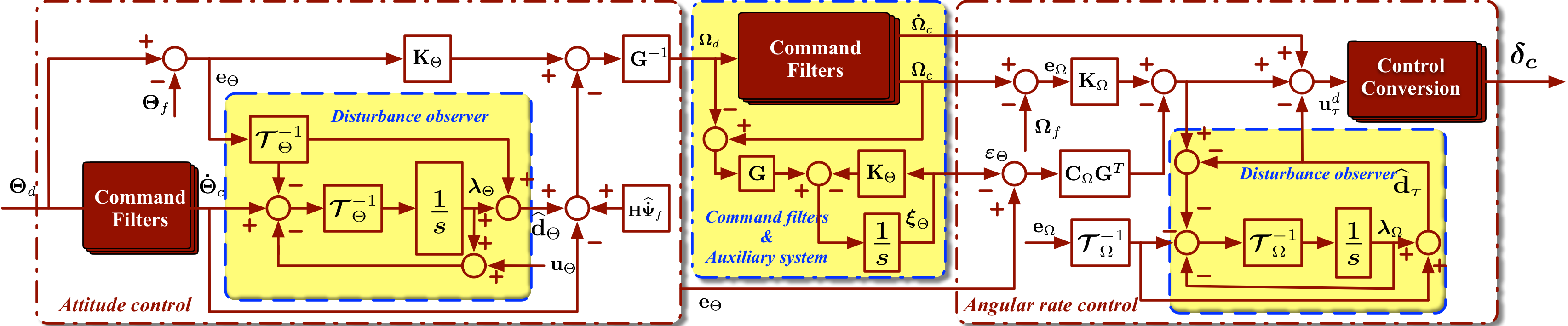
Figure 5: The inner-loop attitude control structure

The uncertainty and disturbance estimator for 𝐝τ\mathbf{d_{\tau}} is given by

𝐝^τ=𝝀Ω+𝓣Ω−1​𝐞Ω​, 𝝀˙Ω=−𝓣Ω−1​𝝀Ω−𝓣Ω−1​(𝓣Ω−1​𝐞Ω−𝐊Ω​𝐞Ω−𝐂Ω​𝐆T​𝜺Θ−𝐝^τ)\mathbf{\widehat{d}_{\tau}}=\boldsymbol{\lambda}_{\Omega}+\boldsymbol{\mathcal{T}}_{\Omega}^{-1}\mathbf{{e}}_{\Omega}\text{, }\quad\boldsymbol{\dot{\lambda}}_{\Omega}=-\boldsymbol{\mathcal{T}}_{\Omega}^{-1}\boldsymbol{\lambda}_{\Omega}-\boldsymbol{\mathcal{T}}_{\Omega}^{-1}\left(\boldsymbol{\mathcal{T}}_{\Omega}^{-1}\mathbf{{e}}_{\Omega}-\mathbf{K}_{\Omega}{\mathbf{e}}_{\Omega}-\mathbf{C}_{\Omega}\mathbf{G}^{T}\boldsymbol{\varepsilon}_{\Theta}-\mathbf{\widehat{d}_{\tau}}\right) (41)

where 𝓣Ω=d​i​a​g​{𝒯p​, ​𝒯q​, ​𝒯r}>0\boldsymbol{\mathcal{T}}_{\Omega}=diag\left\{\mathcal{T}_{p}\text{, }\mathcal{T}_{q}\text{, }\mathcal{T}_{r}\right\}>0 is the time constant matrix. Let 𝜹𝒄=[δa​c​, ​δe​c​, ​δr​c]T\boldsymbol{\delta_{c}}=\left[\delta_{ac}\text{, }\delta_{ec}\text{, }\delta_{rc}\right]^{T} be the commanded control surface deflection vector. Eventually, we have

𝜹𝒄=𝐌¯τ−1​(𝐈𝐮τd+𝛀×𝐈​𝛀−𝝉¯0)\boldsymbol{\delta_{c}}=\mathbf{\overline{M}_{\tau}}^{-1}\left(\mathbf{I}\mathbf{u}_{\tau}^{d}+\boldsymbol{\Omega}\times\mathbf{I}\boldsymbol{\Omega}-\boldsymbol{\overline{\tau}}_{0}\right)\vskip-8.53581pt (42)

The inner-loop controller is shown in Figure 5. The following assumption is introduced for the sake of stability analysis.

Assumption 5.

Both 𝐝Θ\mathbf{d}_{\Theta} and 𝐝τ\boldsymbol{d}_{\tau} are bounded with slow dynamics, namely 𝐝˙Θ≃0\mathbf{\dot{d}}_{\Theta}\simeq 0 and 𝐝˙τ≃0\mathbf{\dot{d}}_{\tau}\simeq 0.

Define 𝐝~Θ=𝐝^Θ−𝐝Θ\mathbf{\widetilde{d}}_{\Theta}=\mathbf{\widehat{d}}_{\Theta}-\mathbf{d}_{\Theta} and 𝐝~τ=𝐝^τ−𝐝τ\mathbf{\widetilde{d}}_{\tau}=\mathbf{\widehat{d}}_{\tau}-\mathbf{d}_{\tau}. Under Assumption 5, we have

𝐝~˙Θ=−𝓣Θ−1​𝐝~Θ​, 𝐝~˙τ=−𝓣Ω−1​𝐝~τ\mathbf{\dot{\widetilde{d}}}_{\Theta}=-\boldsymbol{\mathcal{T}}_{\Theta}^{-1}\mathbf{\widetilde{d}}_{\Theta}\text{, }\qquad\mathbf{\dot{\widetilde{d}}}_{\tau}=-\boldsymbol{\mathcal{T}}_{\Omega}^{-1}\mathbf{\widetilde{d}_{\tau}} (43)
Lemma 3.

If Assumption 5 holds, and KμK_{\mu}, KαK_{\alpha}, KβK_{\beta}, KpK_{p}, KqK_{q}, KrK_{r}, 𝒯μ\mathcal{T}_{\mu}, 𝒯α\mathcal{T}_{\alpha}, 𝒯β\mathcal{T}_{\beta}, 𝒯p\mathcal{T}_{p}, 𝒯q\mathcal{T}_{q}, 𝒯r\mathcal{T}_{r}, cpc_{p}, cqc_{q}, and cr>0c_{r}>0, 𝛆Θ\boldsymbol{\varepsilon}_{\Theta} and 𝐞Ω{\mathbf{e}}_{\Omega} will exponentially converge to zero, namely limt→∞𝐞Θ→𝛏Θ\lim_{t\to\infty}{\mathbf{e}}_{\Theta}\to\boldsymbol{\xi}_{\Theta}, and σc−σd=𝒪⁡(1ωσ)\sigma_{c}-\sigma_{d}=\mathcal{O}\left(\frac{1}{\omega_{\sigma}}\right) and ξσ=𝒪⁡(1ωσ){\xi}_{\sigma}=\mathcal{O}\left(\frac{1}{\omega_{\sigma}}\right) with σ∈{p​, ​q​, ​r}\sigma\in\left\{p\text{, }q\text{, }r\right\}, so 𝐞Θ{\mathbf{e}}_{\Theta} is ultimately bounded.

In real implementations, it is only required that 𝐝Θ\mathbf{d}_{\Theta}, 𝒅τ\boldsymbol{d}_{\tau}, and their derivatives are bounded. If 𝐝˙Θ≃0\mathbf{\dot{d}}_{\Theta}\simeq 0 and 𝒅˙τ≃0\boldsymbol{\dot{d}}_{\tau}\simeq 0 fail to exist, ξσ=𝒪⁡(1ωσ){\xi}_{\sigma}=\mathcal{O}\left(\frac{1}{\omega_{\sigma}}\right) still holds uniformly. However, instead of achieving limt→∞𝜺Ω→0\lim_{t\to\infty}\boldsymbol{\varepsilon}_{\Omega}\to 0, we can only ensure ‖𝜺Θ−𝒆¯Θ‖=𝒪⁡(ϵ1)\|{\boldsymbol{\varepsilon}}_{\Theta}-\boldsymbol{\bar{e}}_{\Theta}\|=\mathcal{O}\left(\epsilon_{1}\right) and ‖𝒆Ω−𝒆¯Ω‖=𝒪⁡(ϵ1)\|\boldsymbol{e}_{\Omega}-\boldsymbol{\bar{e}}_{\Omega}\|=\mathcal{O}\left(\epsilon_{1}\right) where ϵ1\epsilon_{1} is a certain positive small value related to the time constants of the disturbance observers (33) and (41), and 𝒆¯Θ\boldsymbol{\bar{e}}_{\Theta} and 𝒆¯Ω\boldsymbol{\bar{e}}_{\Omega} are the attitude tracking errors from the standard backstepping design. The dynamics of 𝒆¯Θ\boldsymbol{\bar{e}}_{\Theta} and 𝒆¯Ω\boldsymbol{\bar{e}}_{\Omega} are shown in (44). Obviously, there exist limt→∞𝒆¯Θ→0\lim_{t\to\infty}\boldsymbol{\bar{e}}_{\Theta}\to 0 and limt→∞𝒆¯Ω→0\lim_{t\to\infty}\boldsymbol{\bar{e}}_{\Omega}\to 0. Since 𝜺Θ=𝒆Θ−𝝃Θ\boldsymbol{\varepsilon}_{\Theta}=\boldsymbol{e}_{\Theta}-\boldsymbol{\xi}_{\Theta}, 𝒆Θ\boldsymbol{{e}}_{\Theta} will be ultimately bounded. This conclusion is summarized in Proposition 1.

𝒆¯˙Θ=−𝐊Θ​𝒆¯Θ+𝐆​𝐞¯Ω​, 𝐞¯˙Ω=−𝐊Ω​𝐞¯Ω−𝐂Ω​𝐆T​𝒆¯Θ\boldsymbol{\dot{\bar{e}}}_{\Theta}=-\mathbf{K}_{\Theta}\boldsymbol{\bar{e}}_{\Theta}+\mathbf{G}\mathbf{\bar{e}}_{\Omega}\text{, }\qquad\mathbf{\dot{\bar{e}}}_{\Omega}=-\mathbf{K}_{\Omega}{\mathbf{\bar{e}}}_{\Omega}-\mathbf{C}_{\Omega}\mathbf{G}^{T}\boldsymbol{\bar{e}}_{\Theta} (44)
Proposition 1.

Assume 𝐝Θ\mathbf{d}_{\Theta}, 𝐝τ\boldsymbol{d}_{\tau}, and their derivatives are bounded. The proposed inner-loop attitude control law composed of (32), (33), (34), (35), (39), and (41) will make ‖𝛆Θ−𝐞¯Θ‖=𝒪⁡(ϵ1)\|{\boldsymbol{\varepsilon}}_{\Theta}-\boldsymbol{\bar{e}}_{\Theta}\|=\mathcal{O}\left(\epsilon_{1}\right) and ‖𝐞Ω−𝐞¯Ω‖=𝒪⁡(ϵ1)\|\boldsymbol{e}_{\Omega}-\boldsymbol{\bar{e}}_{\Omega}\|=\mathcal{O}\left(\epsilon_{1}\right) uniformly hold, where ϵ1=max⁡{𝒯μ​, ​𝒯α​, ​𝒯β​, ​𝒯p​, ​𝒯q​, ​𝒯r}\epsilon_{1}=\max\left\{\mathcal{T}_{\mu}\text{, }\mathcal{T}_{\alpha}\text{, }\mathcal{T}_{\beta}\text{, }\mathcal{T}_{p}\text{, }\mathcal{T}_{q}\text{, }\mathcal{T}_{r}\right\}. Furthermore, 𝐞Θ\boldsymbol{e}_{\Theta} will be uniformly ultimately bounded, and ‖𝐞Θ−𝐞¯Θ‖=𝒪⁡(ϵ2)\|{\boldsymbol{e}}_{\Theta}-\boldsymbol{\bar{e}}_{\Theta}\|=\mathcal{O}\left(\epsilon_{2}\right) where ϵ2=max⁡{ϵ1​, ​1ωp​, ​1ωq​, ​1ωr}\epsilon_{2}=\max\left\{\epsilon_{1}\text{, }\frac{1}{\omega_{p}}\text{, }\frac{1}{\omega_{q}}\text{, }\frac{1}{\omega_{r}}\right\}.

V Simulation verification

The proposed robust nonlinear close formation controller is validated based on two F-16 aircraft. A high-fidelity model presented in Russel2003Tech will be employed to simulate the nonlinear dynamics of a F-16 aircraft. The aerodynamic effects by close formation flight are characterized using the aerodynamic model developed in Zhang2017JA. Note that the aerodynamic data used to build up the nonlinear aircraft model are assumed to be unavailable for the control design. Instead, a global nonlinear parameter modeling technique in Morelli1998ACC is employed to calculate the necessary aerodynamic coefficients and D¯\overline{D}, L¯0\overline{L}_{0}, L¯α\overline{L}_{\alpha}, 𝝉¯0\boldsymbol{\overline{\tau}}_{0}, and 𝐌¯τ\mathbf{\overline{M}_{\tau}}. The aircraft geometry and mass parameters are listed in Table 1, while the necessary aerodynamic parameters are given in Table 2. The numerical simulations are carried out at two scenarios. In the first scenario, the robustness of the disturbance observer-based controller is verified by being compared with the control without disturbance observers (DO). In the second scenario, close formation flight is conducted at different velocities with the same group of control parameters to further confirm the efficacy of the proposed design.

Table 1: Aircraft geometry and mass parameters
Parameter Symbol Value Unit Parameter Symbol Value Unit
Wing area SS 27.8727.87 m2m^{2} Vertical tail height hth_{t} 3.053.05 mm
Vertical tail area SvS_{v} 5.095.09 m2m^{2} Quarter-chord sweep angle Λs\Lambda_{s} 0.570.57 r​a​drad
Horizontal tail area ShS_{h} 10.03410.034 m2m^{2} Dihedral angle Λd\Lambda_{d} 00 r​a​drad
Wing span bb 9.149.14 mm Gross mass mm 9295.449295.44 k​gkg
Tail wing span btb_{t} 5.495.49 mm Roll moment of inertia IxI_{x} 12874.812874.8 k​g⋅m2kg\cdot m^{2}
Mean aerodynamic chord c¯\bar{c} 3.453.45 mm Pitch moment of inertia IyI_{y} 75673.675673.6 k​g⋅m2kg\cdot m^{2}
Root chord crc_{r} 5.025.02 mm Yaw moment of inertia IzI_{z} 85552.185552.1 k​g⋅m2kg\cdot m^{2}
Tip chord ctc_{t} 1.071.07 mm Product moment of inertia Ix​zI_{xz} 1331.41331.4 k​g⋅m2kg\cdot m^{2}
Table 2: Aircraft aerodynamic coefficients
Coefficient Symbol Value Coefficient Symbol Value
Zero-lift drag coefficient CD0C_{D_{0}} 0.020.02 Rolling moment coefficient CℒδrC_{\mathcal{L}_{\delta_{r}}} 0.026360.02636
Oswald efficiency number eoe_{o} 0.6630.663 Pitching moment coefficient Cℳ0C_{\mathcal{M}_{0}} −0.02029-0.02029
Section lift curve slope ClαC_{l_{\alpha}} 5.35.3 Pitch stiffness CℳαC_{\mathcal{M}_{\alpha}} 0.04660.0466
Lift coefficient CL0C_{L_{0}} 0.050.05 Pitch damping CℳqC_{\mathcal{M}_{q}} −5.159-5.159
Wing lift curve slope CLαC_{L_{\alpha}} 5.35.3 Pitching moment coefficient CℳδeC_{\mathcal{M}_{\delta_{e}}} −0.60123-0.60123
Vertical tail efficiency factor cηc_{\eta} 0.950.95 Weathercock stability derivative C𝒩βC_{\mathcal{N}_{\beta}} 0.29930.2993
Dihedral effect CℒβC_{\mathcal{L}_{\beta}} −0.1059-0.1059 Cross coupling derivative C𝒩pC_{\mathcal{N}_{p}} 0.026780.02678
Roll damping coefficient CℒpC_{\mathcal{L}_{p}} −0.4127-0.4127 Yaw damping coefficient C𝒩rC_{\mathcal{N}_{r}} −0.36988-0.36988
Vertical tail effect coefficient CℒrC_{\mathcal{L}_{r}} 0.06250.0625 Yawing moment coefficient C𝒩δaC_{\mathcal{N}_{\delta_{a}}} −0.03349-0.03349
Rolling moment coefficient CℒδaC_{\mathcal{L}_{\delta_{a}}} −0.1463-0.1463 Yawing moment coefficient C𝒩δrC_{\mathcal{N}_{\delta_{r}}} −0.081159-0.081159
Table 3: Command filter parameters for 𝐋c\mathbf{L}_{c} and χ˙r\dot{\chi}_{r}
Natural frequency Value Damping ratio Value Natural frequency Value Damping ratio Value
ωlx\omega_{l_{x}} 5 ζlx\zeta_{l_{x}} 1 ωly\omega_{l_{y}} 5 ζly\zeta_{l_{y}} 1
ωlz\omega_{l_{z}} 5 ζlz\zeta_{l_{z}} 1 ωχr\omega_{\chi_{r}} 5 ζχr\zeta_{\chi_{r}} 1
Table 4: Outerloop control parameters
Parameter Symbol Value Parameter Symbol Value Parameter Symbol Value
Time constant 𝒯W​x\mathcal{T}_{Wx} 0.80.8 Control gain KxK_{x} 0.30.3 Control gain CyC_{y} 10−410^{-4}
Time constant 𝒯W​y\mathcal{T}_{Wy} 0.50.5 Control gain KzK_{z} 0.20.2 Control gain CzC_{z} 5×10−75\times 10^{-7}
Time constant 𝒯W​z\mathcal{T}_{Wz} 0.40.4 Control gain KVK_{V} 1.751.75 Natural frequency ωV\omega_{V} 88
Time constant 𝒯V\mathcal{T}_{V} 0.250.25 Control gain KγK_{\gamma} 0.750.75 Natural frequency ωγ\omega_{\gamma} 88
Time constant 𝒯γ\mathcal{T}_{\gamma} 0.20.2 Control gain KχK_{\chi} 1.751.75 Damping ratio ζV\zeta_{V} 11
Time constant 𝒯χ\mathcal{T}_{\chi} 0.20.2 Control gain CxC_{x} 10−510^{-5} Damping ratio ζγ\zeta_{\gamma} 11

V.1 Scenario 1: With/without disturbance observers

The initial conditions of the leader aircraft are xl​(0)=45x_{l}\left(0\right)=45 mm, yl=−15y_{l}=-15 mm, zl=−5015z_{l}=-5015 mm, Vl=200V_{l}=200 m/sm/s, γl=χl=0\gamma_{l}=\chi_{l}=0 d​e​gdeg. According to the aerodynamic analysis in Zhang2017JA, the optimal relative position vector is selected to be [−36​, ​9​, ​0]T\left[-36\text{, }9\text{, }0\right]^{T} mm. The parameters of the command filters for generating 𝐋c\mathbf{L}_{c} and estimating are given in Table 3. The initial conditions for the follower aircraft are xf​(0)=45x_{f}\left(0\right)=45 mm, yf​(0)=−15y_{f}\left(0\right)=-15 mm, zf​(0)=−5015z_{f}\left(0\right)=-5015 mm, Vf​(0)=200V_{f}\left(0\right)=200 m/sm/s, γf​(0)=χf​(0)=μf​(0)=βf​(0)=0\gamma_{f}\left(0\right)=\chi_{f}\left(0\right)=\mu_{f}\left(0\right)=\beta_{f}\left(0\right)=0 d​e​gdeg, αf​(0)=2.774\alpha_{f}\left(0\right)=2.774 d​e​gdeg, p=q=r=0p=q=r=0 r​a​d/srad/s. The outerloop and innerloop control parameters are presented in Table 4 and 5, respectively. The formation trajectory in the inertial frame is illustrated in Figures 6. From 00 to 3535 seconds, the formation trajectory is at level and straight flight. From 3535 to 145145 seconds, aircraft in close formation are required to make a turn, and meanwhile reduce their altitudes. After 145145 seconds, level and straight trajectory is recovered. Shown in Figure 7 are the postures and relative positions of the leader and follower aircraft at four different time instants under the proposed robust nonlinear control. The follower aircraft is initially far away from its optimal position relative to the leader aircraft. Under the proposed robust nonlinear controller, the follower aircraft is able to quickly catch up the optimal relative position. Shown in Figure 8 are highlights of the top and front views of the relative positions between the leader and follower aircraft at 180180 seconds.

Table 5: Innerloop control parameters
Parameter Symbol Value Parameter Symbol Value Parameter Symbol Value
Time constant 𝒯μ\mathcal{T}_{\mu} 0.80.8 Control gain KpK_{p} 1212 Natural frequency ωq\omega_{q} 55
Time constant 𝒯α\mathcal{T}_{\alpha} 0.80.8 Control gain KqK_{q} 7.57.5 Natural frequency ωr\omega_{r} 55
Time constant 𝒯β\mathcal{T}_{\beta} 0.80.8 Control gain KrK_{r} 7.57.5 Damping ratio ζμ\zeta_{\mu} 11
Time constant 𝒯p\mathcal{T}_{p} 0.020.02 Control gain cpc_{p} 10−510^{-5} Damping ratio ζα\zeta_{\alpha} 11
Time constant 𝒯q\mathcal{T}_{q} 0.020.02 Natural frequency ωα\omega_{\alpha} 88 Damping ratio ζp\zeta_{p} 11
Time constant 𝒯r\mathcal{T}_{r} 0.020.02 Natural frequency ωμ\omega_{\mu} 88 Damping ratio ζq\zeta_{q} 11
Control gain KμK_{\mu} 55 Control gain crc_{r} 10−510^{-5} Damping ratio ζr\zeta_{r} 11
Control gain KαK_{\alpha} 55 Control gain cqc_{q} 10−510^{-5}
Control gain KβK_{\beta} 55 Natural frequency ωp\omega_{p} 2525
Refer to caption
Figure 6: Formation trajectory
Refer to caption Refer to caption
Figure 7: Aircraft relative positions and postures at different time instants
Refer to caption Refer to caption
Figure 8: Top and front view of close formation flight at t=180t=180 ss

Two different nonlinear controllers are implemented in the first scenario. One is the proposed robust nonlinear formation controller, the other one is purely the baseline nonlinear formation controller without including disturbance observers (DO). The position tracking errors under the two controllers are shown in Figures 9, 10, and 11. According to Zhang2017JA, close formation flight will fail if the optimal lateral and vertical relative positions cannot be tracked with in 10%10\% wing span, while 90%90\% of the maximum drag reduction could be retained if the position tracking error is kept under 5%5\% wing span. For efficient close formation flight, it is required that both the lateral and vertical tracking errors are smaller than at least 5%5\% wing span. To show the validness of the proposed design, the regions covered by 5%5\% and 10%10\% wing span are highlighted in Figures 10 and 11. Obviously, the nonlinear control without including disturbance observers failed to achieve reasonable close formation flight, as the vertical position tracking errors are much far away from the region of interest. After incorporating disturbance observers (DO), both the lateral and vertical position tracking errors are confined to be smaller than 5%5\% wing span, so accurate close formation flight is fulfilled. Furthermore, position tracking errors under the proposed robust nonlinear controller would converge to zero when close formation is at level and straight flight. When the leader aircraft is taking maneuvers (3535 to 145145 ss), steady tracking errors are observed for lateral position tracking. The steady tracking errors are under 5%5\% wing span, which implies efficient close formation flight is still guaranteed. Shown in Figures 12, 13, and 14 are tracking errors of speed, flight path angle, and heading angle, respectively. The non-zero lateral steady tracking errors from 3535 to 145145 ss result from the non-zero tracking errors in heading angle control as shown in Figure 14. When leader aircraft is taking maneuvers, the heading angle will have non-zero tracking errors due to the difference between χ˙r\dot{\chi}_{r} and χ^˙r\dot{\hat{\chi}}_{r}. In real implementations, the derivative of the reference heading angle χr\chi_{r} is always unavailable, so a second order filter is introduced to approximate χ˙r\dot{\chi}_{r}. When the leader aircraft is under level and straight flight, χr\chi_{r} is constant, which implies χ˙r≡0\dot{\chi}_{r}\equiv 0. In this case, χ^˙r\dot{\hat{\chi}}_{r} could be ensured to be equal to χ˙r\dot{\chi}_{r}, so asymptotical stability is able to be obtained as shown in Figures 9, 10, 11, and 14. However, when the leader aircraft is taking maneuvers, χr\chi_{r} is not constant, and χ^˙r\dot{\hat{\chi}}_{r} can only be guaranteed to converge to a certain value close to χ˙r\dot{\chi}_{r}. The difference between χ^˙r\dot{\hat{\chi}}_{r} and χ˙r\dot{\chi}_{r} might lead to the steady heading tracking errors from 3535 to 145145 ss as shown in Figure 14, which is reflected in lateral position tracking control as given in Figure 10.


Figure 9: Longitudinal tracking errors, xe=xf−xrx_{e}=x_{f}-x_{r} (Scenario 1)

Figure 10: Lateral tracking errors, ye=yf−yry_{e}=y_{f}-y_{r} (Scenario 1)

Figure 11: Vertical tracking errors, ze=zf−zrz_{e}=z_{f}-z_{r} (Scenario 1)

The inner-loop state responses are summarized in Figure 15. The sideslip angle of the follower aircraft is always kept to be zero by the proposed robust nonlinear formation controller. Shown in Figure 16 are responses of control inputs. As mentioned before, the baseline formation controller without disturbance observers cannot achieve successful close formation flight. The follower aircraft under the baseline controller is eventually one span away from its optimal relative position to the leader aircraft, in which case the influence of the trailing vortices is quite small. Therefore, the steady performance of the follower aircraft by the baseline formation controller is similar to that of an aircraft at solo flight. Compared with the baseline controller, the robust nonlinear controller will eventually have 13.876%13.876\% decrease in throttle inputs, which implies that around 13.876%13.876\% energy saving could be obtained by close formation flight.


Figure 12: Speed tracking errors, Ve=Vf−VrV_{e}=V_{f}-V_{r} (Scenario 1)

Figure 13: Flight path angle tracking errors, γe=γf−γr\gamma_{e}=\gamma_{f}-\gamma_{r} (Scenario 1)

Figure 14: Heading angle tracking errors, χe=χf−χr\chi_{e}=\chi_{f}-\chi_{r} (Scenario 1)
Figure 15: Inner-loop state responses (Scenario 1)
Figure 16: Actuator responses (Scenario 1)

V.2 Scenario 2: Different flight speeds

The efficacy of the proposed robust nonlinear controller is further verified by running the close formation flight under different velocities. All the control parameters, the reference trajectories, and the initial conditions will be same as those at the first scenario. Without loss of generality, only position tracking errors and control input responses are given. As compared with a linear controller, nonlinear formation controller can be applied to much wider flight scenarios with stability and performance guaranty. This advantage of the nonlinear controller is demonstrated in Figure 17, 18, and 19. It is observed that the proposed robust nonlinear controller is able to ensure almost the same control performance under different velocities. The control input responses under different velocities are illustrated in Figure 20. Another interesting observation is that increasing speed will result in better performance in lateral position tracking as shown in Figure 18. Explaining this observation is difficult from the nonlinear perspective, but we could analyze it from a linear method at a special case. Assume Vf=Vr=C​o​n​s​tV_{f}=V_{r}=Const, γf=γr=0\gamma_{f}=\gamma_{r}=0, and χr=0\chi_{r}=0. The nonlinear closed outer-loop lateral dynamics are linearized about its equilibrium, which results in

y˙e=Vf​eχ​, e˙χ=−Kχ2​eχ−cy​Vf​ye+dχ\dot{y}_{e}=V_{f}e_{\chi}\text{, }\quad\dot{e}_{\chi}=-\frac{K_{\chi}}{2}{e}_{\chi}-c_{y}V_{f}y_{e}+d_{\chi} (45)

where dχd_{\chi} denotes any uncertainties, disturbances, or inputs. The transfer function from dχd_{\chi} to ye{y}_{e} is

G⁡(s)=1s2+Kχ2​s+cy​Vf2G\left(s\right)=\frac{1}{s^{2}+\frac{K_{\chi}}{2}s+c_{y}V_{f}^{2}} (46)

According to the final value theorem, the increase of VfV_{f} leads to smaller steady values in ye{y}_{e} as illustrated in Figure 18.


Figure 17: Longitudinal tracking errors, xe=xf−xrx_{e}=x_{f}-x_{r} (Scenario 2)
Refer to caption
Figure 18: Lateral tracking errors, ye=yf−yry_{e}=y_{f}-y_{r} (Scenario 2)

Figure 19: Vertical tracking errors, ze=zf−zrz_{e}=z_{f}-z_{r} (Scenario 2)
Figure 20: Actuator responses (Scenario 2)

VI Conclusions

The paper presented a robust nonlinear controller for autonomous close formation flight under different flight maneuvers. The proposed controller was developed by combining the command filtered backstepping method and the disturbance observation technique. Both inner-loop and outer-loop controllers were designed in this paper. Based on the proposed design, a follower aircraft is able to track its optimal relative position to a leader aircraft under different flight maneuvers. The proposed design was able to be extended to close formation flight of more than three aircraft, though it was described in the scenario of two-aircraft close formation. Enough robustness and high accuracy could be achieved by the presented design. Different numerical simulations were conducted to demonstrate the efficacy of the presented robust nonlinear close formation controller.

Appendix A: Proof of Lemma 1

For (2), the error dynamic equation is

d~˙=−1𝒯d​d~+d˙\dot{\widetilde{d}}=-\frac{1}{\mathcal{T}_{d}}\widetilde{d}+\dot{d} (47)

By solving the first-order differential equation (47), one has d~​(t)=e−t𝒯d​d~​(0)+∫0te−t−τ𝒯d​d˙​(τ)​𝑑τ\widetilde{d}\left(t\right)=e^{-\frac{t}{\mathcal{T}_{d}}}\widetilde{d}\left(0\right)+\int_{0}^{t}e^{-\frac{t-\tau}{\mathcal{T}_{d}}}\dot{d}\left(\tau\right)d\tau. If choosing d^​(0)=0\widehat{d}\left(0\right)=0, we have d~​(0)=−d​(0)\widetilde{d}\left(0\right)=-{d}\left(0\right). If d˙​(t)∈ℒ∞\dot{d}\left(t\right)\in\mathscr{L}_{\infty},

|d~​(t)|≤e−t𝒯d​|d⁡(0)|+∫0te−t−τ𝒯d​𝑑τ​‖d˙‖∞≤e−t𝒯d​|d⁡(0)|+𝒯d​(1−e−t𝒯d)​‖d˙‖∞|\widetilde{d}\left(t\right)|\leq e^{-\frac{t}{\mathcal{T}_{d}}}|{d}\left(0\right)|+\int_{0}^{t}e^{-\frac{t-\tau}{\mathcal{T}_{d}}}d\tau\|\dot{d}\|_{\infty}\leq e^{-\frac{t}{\mathcal{T}_{d}}}|{d}\left(0\right)|+\mathcal{T}_{d}\left(1-e^{-\frac{t}{\mathcal{T}_{d}}}\right)\|\dot{d}\|_{\infty} (48)

Obviously, |d~|≤max⁡{|d⁡(0)|​, ​𝒯d​‖d˙‖∞}|\widetilde{d}|\leq\max\left\{|{d}\left(0\right)|\text{, }\mathcal{T}_{d}\|\dot{d}\|_{\infty}\right\} globally exists.

For any positive constant ϵ\epsilon, if 𝒯d​‖d˙‖∞+ϵ>|d⁡(0)|\mathcal{T}_{d}\|\dot{d}\|_{\infty}+\epsilon>|{d}\left(0\right)|, there exists |d~|<𝒯d​‖d˙‖∞+ϵ|\widetilde{d}|<\mathcal{T}_{d}\|\dot{d}\|_{\infty}+\epsilon ∀tϵ>0\forall t_{\epsilon}>0 according to the global boundedness of |d~||\widetilde{d}|. If 𝒯d​‖d˙‖∞+ϵ<|d⁡(0)|\mathcal{T}_{d}\|\dot{d}\|_{\infty}+\epsilon<|{d}\left(0\right)|, the first term on the right-hand side of (48) will decrease, while the second term will increase. At certain time tϵt_{\epsilon}, there exists e−t𝒯d​|d⁡(0)|+𝒯d​(1−e−t𝒯d)​‖d˙‖∞=𝒯d​‖d˙‖∞+ϵe^{-\frac{t}{\mathcal{T}_{d}}}|{d}\left(0\right)|+\mathcal{T}_{d}\left(1-e^{-\frac{t}{\mathcal{T}_{d}}}\right)\|\dot{d}\|_{\infty}=\mathcal{T}_{d}\|\dot{d}\|_{\infty}+\epsilon. After tϵt_{\epsilon}, the right hand side of (48) will be smaller than 𝒯d​‖d˙‖∞+ϵ\mathcal{T}_{d}\|\dot{d}\|_{\infty}+\epsilon. By simple mathematical calculation, one has tϵ=𝒯d​ln⁡(||d⁡(0)|−𝒯d​‖d˙‖∞|ϵ)t_{\epsilon}=\mathcal{T}_{d}\ln\left(\frac{||{d}\left(0\right)|-\mathcal{T}_{d}\|\dot{d}\|_{\infty}|}{\epsilon}\right), so the second conclusion of Lemma 1 is obtained. In addition, the estimator error is input-to-state stable with respect to d˙\dot{d} according to (47). Hence, it is obvious that limt→∞d~=0\lim_{t\to\infty}\widetilde{d}=0, if limt→∞d˙=0\lim_{t\to\infty}\dot{d}=0.

Appendix B: Proof of Lemma 2

The following error dynamics are easy to obtain.

𝐞˙𝒮=𝐀𝒮​𝐞𝒮+𝐁𝒮​(𝒮¨+2​ζ𝒮​ω𝒮​𝒮˙)\dot{\mathbf{e}}_{\mathscr{S}}=\mathbf{A}_{\mathscr{S}}\mathbf{e}_{\mathscr{S}}+\mathbf{B}_{\mathscr{S}}\left(\ddot{\mathscr{S}}+2\zeta_{\mathscr{S}}\omega_{\mathscr{S}}\dot{\mathscr{S}}\right) (49)

where 𝐁𝒮=[0​, −1]T\mathbf{B}_{\mathscr{S}}=\left[0\text{, }-1\right]^{T}. By choosing ζ𝒮​, ​ω𝒮>0\zeta_{\mathscr{S}}\text{, }\omega_{\mathscr{S}}>0, 𝐀𝒮\mathbf{A}_{\mathscr{S}} is Hurwitz, which implies 𝐏𝒮​𝐀𝒮+𝐀𝒮T​𝐏𝒮=−𝐈\mathbf{P}_{\mathscr{S}}\mathbf{A}_{\mathscr{S}}+\mathbf{A}^{T}_{\mathscr{S}}\mathbf{P}_{\mathscr{S}}=-\mathbf{I} with 𝐏𝒮>0\mathbf{P}_{\mathscr{S}}>0. Choose 𝕍=𝐞𝒮T​𝐏𝒮​𝐞𝒮\mathbb{V}=\mathbf{e}_{\mathscr{S}}^{T}\mathbf{P}_{\mathscr{S}}\mathbf{e}_{\mathscr{S}} as the Lyapunov function for (49), so

λm​i​n​(𝐏𝒮)​‖𝐞𝒮‖22≤𝕍≤λm​a​x​(𝐏𝒮)​‖𝐞𝒮‖22\lambda_{min}\left(\mathbf{P}_{\mathscr{S}}\right)\|\mathbf{e}_{\mathscr{S}}\|_{2}^{2}\leq\mathbb{V}\leq\lambda_{max}\left(\mathbf{P}_{\mathscr{S}}\right)\|\mathbf{e}_{\mathscr{S}}\|_{2}^{2} (50)

If both 𝒮¨\ddot{\mathscr{S}} and 𝒮˙\dot{\mathscr{S}} are bounded, differentiating 𝕍\mathbb{V} with respect to time will yield

𝕍˙=𝐞𝒮T​(𝐏𝒮​𝐀𝒮+𝐀𝒮T​𝐏𝒮)​𝐞𝒮+2​𝐞𝒮T​𝐏𝒮​𝐁𝒮​(𝒮¨+2​ζ𝒮​ω𝒮​𝒮˙)≤−𝕍λm​a​x​(𝐏𝒮)+2​λm​a​x​(𝐏𝒮)λm​i​n​(𝐏𝒮)​‖𝒮¨+2​ζ𝒮​ω𝒮​𝒮˙‖∞​𝕍\begin{array}[]{ll}\dot{\mathbb{V}}&=\mathbf{e}_{\mathscr{S}}^{T}\left(\mathbf{P}_{\mathscr{S}}\mathbf{A}_{\mathscr{S}}+\mathbf{A}_{\mathscr{S}}^{T}\mathbf{P}_{\mathscr{S}}\right)\mathbf{e}_{\mathscr{S}}+2\mathbf{e}_{\mathscr{S}}^{T}\mathbf{P}_{\mathscr{S}}\mathbf{B}_{\mathscr{S}}\left(\ddot{\mathscr{S}}+2\zeta_{\mathscr{S}}\omega_{\mathscr{S}}\dot{\mathscr{S}}\right)\\ &\leq-\frac{\mathbb{V}}{\lambda_{max}\left(\mathbf{P}_{\mathscr{S}}\right)}+\frac{2\lambda_{max}\left(\mathbf{P}_{\mathscr{S}}\right)}{\sqrt{\lambda_{min}\ \left(\mathbf{P}_{\mathscr{S}}\right)}}\|\ddot{\mathscr{S}}+2\zeta_{\mathscr{S}}\omega_{\mathscr{S}}\dot{\mathscr{S}}\|_{\infty}\sqrt{\mathbb{V}}\end{array}

Let 𝕎⁡(t)=𝕍\mathbb{W}\left(t\right)=\sqrt{\mathbb{V}}, so 𝕎˙=𝕍˙2​𝕍\dot{\mathbb{W}}=\frac{\dot{\mathbb{V}}}{2\sqrt{\mathbb{V}}}, when 𝕍≠0\mathbb{V}\neq 0. Hence, 𝕎˙≤−𝕎/(2λm​a​x(𝐏𝒮))+λm​a​x(𝐏𝒮)∥𝒮¨+2ζ𝒮ω𝒮𝒮˙∥∞/λm​i​n​(𝐏𝒮)\dot{\mathbb{W}}\leq-{\mathbb{W}}\left/{\left(2\lambda_{max}\left(\mathbf{P}_{\mathscr{S}}\right)\right)}\right.+{\lambda_{max}\left(\mathbf{P}_{\mathscr{S}}\right)}\|\ddot{\mathscr{S}}+2\zeta_{\mathscr{S}}\omega_{\mathscr{S}}\dot{\mathscr{S}}\|_{\infty}\left/{\sqrt{\lambda_{min}\left(\mathbf{P}_{\mathscr{S}}\right)}}\right.. According to the comparison principle (Page 102, Khalil2002Book), one can get

𝕎≤e−t2​λm​a​x​(𝐏𝒮)​𝕎​(0)+(1−e−t2​λm​a​x​(𝐏𝒮))​2​λm​a​x2​(𝐏)λm​i​n​(𝐏)​‖𝒮¨+2​ζ𝒮​ω𝒮​𝒮˙‖∞\begin{array}[]{ll}\mathbb{W}&\leq e^{-\frac{t}{2\lambda_{max}\left(\mathbf{P}_{\mathscr{S}}\right)}}\mathbb{W}\left(0\right)+\left(1-e^{-\frac{t}{2\lambda_{max}\left(\mathbf{P}_{\mathscr{S}}\right)}}\right)\frac{2\lambda^{2}_{max}\left(\mathbf{P}\right)}{\sqrt{\lambda_{min}\left(\mathbf{P}\right)}}\|\ddot{\mathscr{S}}+2\zeta_{\mathscr{S}}\omega_{\mathscr{S}}\dot{\mathscr{S}}\|_{\infty}\end{array}

According to (50), 𝕎≤λm​a​x​(𝐏𝒮)​‖𝐞𝒮‖2\mathbb{W}\leq\sqrt{\lambda_{max}\left(\mathbf{P}_{\mathscr{S}}\right)}\|\mathbf{e}_{\mathscr{S}}\|_{2}, so 𝕎⁡(0)≤λm​a​x​(𝐏𝒮)​‖𝐞𝒮​(0)‖2\mathbb{W}\left(0\right)\leq\lambda_{max}\left(\mathbf{P}_{\mathscr{S}}\right)\|\mathbf{e}_{\mathscr{S}}\left(0\right)\|_{2}. By setting 𝒮c​(0)=𝒮​(0)\mathscr{S}_{c}\left(0\right)=\mathscr{S}\left(0\right), and 𝒮˙c​(0)=0\dot{\mathscr{S}}_{c}\left(0\right)=0, one has ‖𝐞𝒮​(0)‖=|𝒮˙​(0)|\|\mathbf{e}_{\mathscr{S}}\left(0\right)\|=|\dot{\mathscr{S}}\left(0\right)|. Eventually,

‖𝐞𝒮‖2≤λm​a​x​(𝐏𝒮)λm​i​n​(𝐏𝒮)​e−t2​λm​a​x​(𝐏𝒮)​|𝒮˙​(0)|+(1−e−t2​λm​a​x​(𝐏𝒮))​2​λm​a​x2​(𝐏𝒮)λm​i​n​(𝐏𝒮)​‖𝒮¨+2​ζ𝒮​ω𝒮​𝒮˙‖∞\footnotesize\|\mathbf{e}_{\mathscr{S}}\|_{2}\leq\sqrt{\frac{\lambda_{max}\left(\mathbf{P_{\mathscr{S}}}\right)}{\lambda_{min}\left(\mathbf{P_{\mathscr{S}}}\right)}}e^{-\frac{t}{2\lambda_{max}\left(\mathbf{P_{\mathscr{S}}}\right)}}|\dot{\mathscr{S}}\left(0\right)|+\left(1-e^{-\frac{t}{2\lambda_{max}\left(\mathbf{P_{\mathscr{S}}}\right)}}\right)\frac{2\lambda_{max}^{2}\left(\mathbf{P}_{\mathscr{S}}\right)}{\lambda_{min}\left(\mathbf{P}_{\mathscr{S}}\right)}\|\ddot{\mathscr{S}}+2\zeta_{\mathscr{S}}\omega_{\mathscr{S}}\dot{\mathscr{S}}\|_{\infty}

Therefore, 𝐞𝒮\mathbf{e}_{\mathscr{S}} is uniformly and ultimately bounded. With the consideration of ‖𝒮~‖2≤‖𝐞𝒮‖2\|\tilde{\mathscr{S}}\|_{2}\leq\|\mathbf{e}_{\mathscr{S}}\|_{2}, we are able to conclude that 𝒮~\tilde{\mathscr{S}} is uniformly and ultimately bounded.

The second conclusion of Lemma 2 could be demonstrated by virtue of the perturbation theory. According to (49), the following singularly perturbed system is readily obtained.

1ω𝒮​𝒮~˙1=𝒮~2​, 1ω𝒮​𝒮~˙2=−2​ζ𝒮​𝒮~2−𝒮~1−1ω𝒮​(1ω𝒮​𝒮¨+2​ζ𝒮​𝒮˙)\small\frac{1}{\omega_{\mathscr{S}}}\dot{\tilde{\mathscr{S}}}_{1}=\tilde{\mathscr{S}}_{2}\text{, }\hskip 18.49988pt\frac{1}{\omega_{\mathscr{S}}}\dot{\tilde{\mathscr{S}}}_{2}=-2\zeta_{\mathscr{S}}\tilde{\mathscr{S}}_{2}-\tilde{\mathscr{S}}_{1}-\frac{1}{\omega_{\mathscr{S}}}\left(\frac{1}{\omega_{\mathscr{S}}}\ddot{\mathscr{S}}+2\zeta_{\mathscr{S}}\dot{\mathscr{S}}\right)

where 𝒮~1=𝒮~\tilde{\mathscr{S}}_{1}=\tilde{\mathscr{S}} and 𝒮~2=1ω𝒮​𝒮~˙\tilde{\mathscr{S}}_{2}=\frac{1}{\omega_{\mathscr{S}}}\dot{\tilde{\mathscr{S}}}. Obviously, the effect of 1ω𝒮​𝒮¨+2​ζ𝒮​𝒮˙\frac{1}{\omega_{\mathscr{S}}}\ddot{\mathscr{S}}+2\zeta_{\mathscr{S}}\dot{\mathscr{S}} will be diminished by increasing the natural frequency ω𝒮\omega_{\mathscr{S}}. According to the properties of singularly perturbed system, we readily have 𝒮~1=𝒮c−𝒮=𝒪⁡(1ω𝒮)\tilde{\mathscr{S}}_{1}=\mathscr{S}_{c}-\mathscr{S}=\mathcal{O}\left(\frac{1}{\omega_{\mathscr{S}}}\right) and 𝒮~˙2=𝒮~˙ω𝒮=𝒪⁡(1ω𝒮)\dot{\tilde{\mathscr{S}}}_{2}=\frac{\dot{\tilde{\mathscr{S}}}}{\omega_{\mathscr{S}}}=\mathcal{O}\left(\frac{1}{\omega_{\mathscr{S}}}\right).

Appendix C: Proof of Lemma 3

In light of (31), (36), (32), (38), (39), (40), and (43), one has

{𝜺˙Θ=−𝐊Θ​𝜺Θ+𝐆𝐞Ω−𝐝~Θ𝐞˙Ω=−𝐊Ω​𝐞Ω−𝐂Ω​𝐆T​𝜺Θ−𝐝~τ{𝐝~˙Θ=−𝓣Θ−1​𝐝~Θ𝐝~˙τ=−𝓣Ω−1​𝐝~τ\left\{\begin{array}[]{ll}\boldsymbol{\dot{\varepsilon}}_{\Theta}&=-\mathbf{K}_{\Theta}\boldsymbol{\varepsilon}_{\Theta}+\mathbf{G}\mathbf{e}_{\Omega}-\mathbf{\widetilde{d}}_{\Theta}\\ \mathbf{\dot{e}}_{\Omega}&=-\mathbf{K}_{\Omega}{\mathbf{e}}_{\Omega}-\mathbf{C}_{\Omega}\mathbf{G}^{T}\boldsymbol{\varepsilon}_{\Theta}-\mathbf{\widetilde{d}_{\tau}}\end{array}\right.\qquad\left\{\begin{array}[]{ll}\mathbf{\dot{\widetilde{d}}}_{\Theta}&=-\boldsymbol{\mathcal{T}}_{\Theta}^{-1}\widetilde{\mathbf{d}}_{\Theta}\\ \mathbf{\dot{\widetilde{d}}}_{\tau}&=-\boldsymbol{\mathcal{T}}_{\Omega}^{-1}\widetilde{\mathbf{d}}_{\tau}\end{array}\right. (51)

The stability of (51) is shown by picking the Lyapunov function 𝕍\mathbb{V} as below.

𝕍=𝜺ΘT​𝜺Θ2+𝐞ΩT​𝐂Ω−1​𝐞Ω2+𝐝~ΘT​𝐝~Θ2+𝐝~τT​𝐂Ω−1​𝐝~τ2\mathbb{V}=\frac{\boldsymbol{\varepsilon}_{\Theta}^{T}\boldsymbol{\varepsilon}_{\Theta}}{2}+\frac{\mathbf{e}_{\Omega}^{T}\mathbf{C}_{\Omega}^{-1}\mathbf{e}_{\Omega}}{2}+\frac{\widetilde{\mathbf{d}}_{\Theta}^{T}\widetilde{\mathbf{d}}_{\Theta}}{2}+\frac{\widetilde{\mathbf{d}}_{\tau}^{T}\mathbf{C}_{\Omega}^{-1}\widetilde{\mathbf{d}}_{\tau}}{2} (52)

The derivative of 𝕍\mathbb{V} is

𝕍˙=𝜺ΘT​(−𝐊Θ​𝜺Θ+𝐆𝐞Ω−𝐝~Θ)−𝐞ΩT​𝐂Ω−1​(𝐊Ω​𝐞Ω+𝐂Ω​𝐆T​𝜺Θ+𝐝~τ)−𝐝~ΘT​𝓣Θ−1​𝐝~Θ−𝐝~τT​𝐂Ω−1​𝓣Ω−1​𝐝~τ=−𝜺ΘT​𝐊Θ​𝜺Θ−𝜺ΘT​𝐝~Θ−𝐞ΩT​𝐂Ω−1​𝐊Ω​𝐞Ω−𝐞ΩT​𝐂τ−1​𝐝~τ−𝐝~ΘT​𝓣Θ−1​𝐝~Θ−𝐝~τT​𝐂Ω−1​𝓣Ω−1​𝐝~τ\small\begin{array}[]{ll}\dot{\mathbb{V}}&=\boldsymbol{\varepsilon}_{\Theta}^{T}\left(-\mathbf{K}_{\Theta}\boldsymbol{\varepsilon}_{\Theta}+\mathbf{G}\mathbf{e}_{\Omega}-\mathbf{\widetilde{d}}_{\Theta}\right)-\mathbf{e}_{\Omega}^{T}\mathbf{C}_{\Omega}^{-1}\left(\mathbf{K}_{\Omega}{\mathbf{e}}_{\Omega}+\mathbf{C}_{\Omega}\mathbf{G}^{T}\boldsymbol{\varepsilon}_{\Theta}+\mathbf{\widetilde{d}_{\tau}}\right)-\mathbf{\widetilde{d}}_{\Theta}^{T}\boldsymbol{\mathcal{T}}_{\Theta}^{-1}\mathbf{\widetilde{d}}_{\Theta}-\mathbf{\widetilde{d}}_{\tau}^{T}\mathbf{C}_{\Omega}^{-1}\boldsymbol{\mathcal{T}}_{\Omega}^{-1}\mathbf{\widetilde{d}}_{\tau}\\ &=-\boldsymbol{\varepsilon}_{\Theta}^{T}\mathbf{K}_{\Theta}\boldsymbol{\varepsilon}_{\Theta}-\boldsymbol{\varepsilon}_{\Theta}^{T}\mathbf{\widetilde{d}}_{\Theta}-\mathbf{e}_{\Omega}^{T}\mathbf{C}_{\Omega}^{-1}\mathbf{K}_{\Omega}{\mathbf{e}}_{\Omega}-\mathbf{e}_{\Omega}^{T}\mathbf{C}_{\tau}^{-1}\mathbf{\widetilde{d}_{\tau}}-\mathbf{\widetilde{d}}_{\Theta}^{T}\boldsymbol{\mathcal{T}}_{\Theta}^{-1}\mathbf{\widetilde{d}}_{\Theta}-\mathbf{\widetilde{d}}_{\tau}^{T}\mathbf{C}_{\Omega}^{-1}\boldsymbol{\mathcal{T}}_{\Omega}^{-1}\mathbf{\widetilde{d}}_{\tau}\end{array}

where 𝐝~Θ\mathbf{\widetilde{d}}_{\Theta} and 𝐝~τ\mathbf{\widetilde{d}}_{\tau} are both vectors. Let 𝐝~Θ=[d~μ​, ​d~α​, ​d~β]T\mathbf{\widetilde{d}}_{\Theta}=\left[\widetilde{d}_{\mu}\text{, }\widetilde{d}_{\alpha}\text{, }\widetilde{d}_{\beta}\right]^{T} and 𝐝~τ=[d~p​, ​d~q​, ​d~r]T\mathbf{\widetilde{d}}_{\tau}=\left[\widetilde{d}_{p}\text{, }\widetilde{d}_{q}\text{, }\widetilde{d}_{r}\right]^{T}, so

𝕍˙\displaystyle\dot{\mathbb{V}} =\displaystyle= −Kμ​εμ2−Kα​εα2−Kβ​εβ2−εμ​d~μ−εα​d~α−εβ​d~β−d~μ2𝒯μ−d~α2𝒯α−d~β2𝒯β\displaystyle-K_{\mu}\varepsilon_{\mu}^{2}-K_{\alpha}\varepsilon_{\alpha}^{2}-K_{\beta}\varepsilon_{\beta}^{2}-\varepsilon_{\mu}\widetilde{d}_{\mu}-\varepsilon_{\alpha}\widetilde{d}_{\alpha}-\varepsilon_{\beta}\widetilde{d}_{\beta}-\frac{\widetilde{d}_{\mu}^{2}}{\mathcal{T}_{\mu}}-\frac{\widetilde{d}_{\alpha}^{2}}{\mathcal{T}_{\alpha}}-\frac{\widetilde{d}_{\beta}^{2}}{\mathcal{T}_{\beta}} (53)
−Kp​ep2cp−Kq​eq2cq−Kr​er2cr−ep​d~pcp−eq​d~qcq−er​d~rcr−d~p2cp​𝒯p−d~q2cq​𝒯q−d~r2cr​𝒯r\displaystyle-\frac{K_{p}e_{p}^{2}}{c_{p}}-\frac{K_{q}e_{q}^{2}}{c_{q}}-\frac{K_{r}e_{r}^{2}}{c_{r}}-\frac{e_{p}\widetilde{d}_{p}}{c_{p}}-\frac{e_{q}\widetilde{d}_{q}}{c_{q}}-\frac{e_{r}\widetilde{d}_{r}}{c_{r}}-\frac{\widetilde{d}_{p}^{2}}{c_{p}\mathcal{T}_{p}}-\frac{\widetilde{d}_{q}^{2}}{c_{q}\mathcal{T}_{q}}-\frac{\widetilde{d}_{r}^{2}}{c_{r}\mathcal{T}_{r}}

It is easy to show that 𝕍˙2\dot{\mathbb{V}}_{2} is negative definite, if all control parameters are chosen to be positive. Hence, 𝜺Θ\boldsymbol{\varepsilon}_{\Theta} and 𝐞Ω{\mathbf{e}}_{\Omega} will exponentially converge to zero. To show the second conclusion in Lemma 3, a singular perturbation model is established based on (35) and (40). To simplify the analysis complexity, assume that ωp=ωq=ωr=ωΩ\omega_{p}=\omega_{q}=\omega_{r}=\omega_{\Omega} and ζp=ζq=ζr=ζΩ\zeta_{p}=\zeta_{q}=\zeta_{r}=\zeta_{\Omega}. Define a new variable 𝛀¯c​d​o​t=𝛀˙cωΩ\boldsymbol{\bar{\Omega}}_{cdot}=\frac{\boldsymbol{\dot{\Omega}}_{c}}{\omega_{\Omega}}. Therefore, the singular perturbation model is

𝝃˙Θ\displaystyle\boldsymbol{\dot{\xi}}_{\Theta} =−𝐊Θ​𝝃Θ+𝐆⁡(𝛀c−𝛀d)\displaystyle=-\mathbf{K}_{\Theta}\boldsymbol{{\xi}}_{{\Theta}}+\mathbf{G}\left(\boldsymbol{\Omega}_{c}-\boldsymbol{\Omega}_{d}\right) (54a)
1ωΩ​𝛀˙c\displaystyle\frac{1}{\omega_{\Omega}}\boldsymbol{\dot{\Omega}}_{c} =𝛀¯c​d​o​t\displaystyle=\boldsymbol{\bar{\Omega}}_{cdot} (54b)
1ωΩ​𝛀¯˙c​d​o​t\displaystyle\frac{1}{\omega_{\Omega}}\boldsymbol{\dot{\bar{\Omega}}}_{cdot} =−2​ζΩωΩ​𝛀¯˙c​d​o​t−(𝛀c−𝛀d)\displaystyle=-\frac{2\zeta_{\Omega}}{\omega_{\Omega}}\boldsymbol{\dot{\bar{\Omega}}}_{cdot}-\left(\boldsymbol{\Omega}_{c}-\boldsymbol{\Omega}_{d}\right) (54c)

Obviously, the command filter system composed of (54b) and (54c) has much faster dynamics than the auxiliary system (54a), if ωΩ\omega_{\Omega} is chosen to be sufficiently large. The reduced system of (54) is given by 𝝃¯˙Θ=−𝐊Θ​𝝃¯Θ\boldsymbol{\dot{\bar{\xi}}}_{\Theta}=-\mathbf{K}_{\Theta}\boldsymbol{\bar{\xi}}_{\Theta} by setting ωΩ\omega_{\Omega} to be infinity, where 𝝃¯Θ\boldsymbol{\bar{\xi}}_{\Theta} is the reduced system state vector. If 𝝃Θ​(0)=𝝃¯Θ​(0)=0\boldsymbol{\xi}_{\Theta}\left(0\right)=\boldsymbol{\bar{\xi}}_{\Theta}\left(0\right)=0, ‖𝝃Θ‖=𝒪⁡(1ωΩ)\|\boldsymbol{\xi}_{\Theta}\|=\mathcal{O}\left(\frac{1}{\omega_{\Omega}}\right) will hold uniformly according to the Tikhonov’s theorem, which implies ξσ=𝒪⁡(1ωσ){\xi}_{\sigma}=\mathcal{O}\left(\frac{1}{\omega_{\sigma}}\right). It is easy to get σc−σd=𝒪⁡(1ωσ)\sigma_{c}-\sigma_{d}=\mathcal{O}\left(\frac{1}{\omega_{\sigma}}\right) according to Lemma 2.

Appendix D: Proof of Proposition 1

When 𝐝˙Θ≠0\mathbf{\dot{d}}_{\Theta}\neq 0 and 𝑫˙τ≠0\boldsymbol{\dot{D}}_{\tau}\neq 0, the closed-loop error dynamics (51) will be rewritten as

{𝜺˙Θ=−𝐊Θ​𝜺Θ+𝐆𝐞Ω−𝐝~Θ𝐞˙Ω=−𝐊Ω​𝐞Ω−𝐂Ω​𝐆T​𝜺Θ−𝐝~τ{𝓣Θ​𝐝~˙Θ=−𝐝~Θ−𝓣Θ​𝐝˙Θ𝓣Ω​𝐝~˙τ=−𝐝~τ−𝓣Ω​𝐝˙τ\left\{\begin{array}[]{ll}\boldsymbol{\dot{\varepsilon}}_{\Theta}&=-\mathbf{K}_{\Theta}\boldsymbol{\varepsilon}_{\Theta}+\mathbf{G}\mathbf{e}_{\Omega}-\mathbf{\widetilde{d}}_{\Theta}\\ \mathbf{\dot{e}}_{\Omega}&=-\mathbf{K}_{\Omega}{\mathbf{e}}_{\Omega}-\mathbf{C}_{\Omega}\mathbf{G}^{T}\boldsymbol{\varepsilon}_{\Theta}-\mathbf{\widetilde{d}_{\tau}}\end{array}\right.\qquad\left\{\begin{array}[]{ll}\boldsymbol{\mathcal{T}}_{\Theta}\mathbf{\dot{\widetilde{d}}}_{\Theta}&=-\mathbf{\widetilde{d}}_{\Theta}-\boldsymbol{\mathcal{T}}_{\Theta}\mathbf{\dot{d}}_{\Theta}\\ \boldsymbol{\mathcal{T}}_{\Omega}\mathbf{\dot{\widetilde{d}}}_{\tau}&=-\mathbf{\widetilde{d}_{\tau}}-\boldsymbol{\mathcal{T}}_{\Omega}\mathbf{\dot{d}}_{\tau}\end{array}\right. (55)

If the time constants 𝓣Θ\boldsymbol{\mathcal{T}}_{\Theta} and 𝓣Ω\boldsymbol{\mathcal{T}}_{\Omega} are chosen to be sufficiently small, (55) will be a standard perturbation model whose reduced system is given in (44). The reduced system (44) is apparently exponentially stable. Since both 𝐝˙Θ\mathbf{\dot{d}}_{\Theta} and 𝑫˙τ\boldsymbol{\dot{D}}_{\tau} are bounded, their impact will be diminished by reducing 𝓣Θ\boldsymbol{\mathcal{T}}_{\Theta} and 𝓣Ω\boldsymbol{\mathcal{T}}_{\Omega}, respectively. Since 𝛀c​(0)=𝛀c​(0)\boldsymbol{\Omega}_{c}\left(0\right)=\boldsymbol{\Omega}_{c}\left(0\right) and 𝝃Θ​(0)=0\boldsymbol{\xi}_{\Theta}\left(0\right)=0, one has 𝜺Θ​(0)=𝒆¯Θ​(0)\boldsymbol{{\varepsilon}}_{\Theta}\left(0\right)=\boldsymbol{\bar{e}}_{\Theta}\left(0\right) and 𝒆Ω​(0)=𝒆¯Ω​(0)\boldsymbol{{e}}_{\Omega}\left(0\right)=\boldsymbol{\bar{e}}_{\Omega}\left(0\right). According to the Tikhonov’s theorem for a standard perturbation model, one is able to conclude that ‖𝜺Θ−𝒆¯Θ‖=𝒪⁡(ϵ1)\|{\boldsymbol{\varepsilon}}_{\Theta}-\boldsymbol{\bar{e}}_{\Theta}\|=\mathcal{O}\left(\epsilon_{1}\right) and ‖𝒆Ω−𝒆¯Ω‖=𝒪⁡(ϵ1)\|\boldsymbol{e}_{\Omega}-\boldsymbol{\bar{e}}_{\Omega}\|=\mathcal{O}\left(\epsilon_{1}\right) will uniformly hold. According to the definition of the oder of magnitude, it is easy to find that ϵ1=max⁡{𝒯μ​, ​𝒯α​, ​𝒯β​, ​𝒯p​, ​𝒯q​, ​𝒯r}\epsilon_{1}=\max\left\{\mathcal{T}_{\mu}\text{, }\mathcal{T}_{\alpha}\text{, }\mathcal{T}_{\beta}\text{, }\mathcal{T}_{p}\text{, }\mathcal{T}_{q}\text{, }\mathcal{T}_{r}\right\}.

Furthermore, with the consideration of (54) and (55), we have

{𝒆˙Θ=−𝐊Θ​𝒆Θ+𝐆𝐞Ω+𝐆⁡(𝛀c−𝛀d)−𝐝~Θ𝐞˙Ω=−𝐊Ω​𝐞Ω−𝐂Ω​𝐆T​(𝒆Θ−𝝃Θ)−𝐝~τ𝝃˙Θ=−𝐊Θ​𝝃Θ+𝐆⁡(𝛀c−𝛀d)\left\{\begin{array}[]{ll}\boldsymbol{\dot{e}}_{\Theta}&=-\mathbf{K}_{\Theta}\boldsymbol{e}_{\Theta}+\mathbf{G}\mathbf{e}_{\Omega}+\mathbf{G}\left(\boldsymbol{\Omega}_{c}-\boldsymbol{\Omega}_{d}\right)-\mathbf{\widetilde{d}}_{\Theta}\\ \mathbf{\dot{e}}_{\Omega}&=-\mathbf{K}_{\Omega}{\mathbf{e}}_{\Omega}-\mathbf{C}_{\Omega}\mathbf{G}^{T}\left(\boldsymbol{e}_{\Theta}-\boldsymbol{\xi}_{\Theta}\right)-\mathbf{\widetilde{d}_{\tau}}\\ \boldsymbol{\dot{\xi}}_{\Theta}&=-\mathbf{K}_{\Theta}\boldsymbol{\xi}_{\Theta}+\mathbf{G}\left(\boldsymbol{\Omega}_{c}-\boldsymbol{\Omega}_{d}\right)\end{array}\right. (56)
{1ωΩ​𝛀˙c=𝛀¯c​d​o​t1ωΩ​𝛀¯˙c​d​o​t=−2​ζΩωΩ​𝛀¯˙c​d​o​t−(𝛀c−𝛀d){𝓣Θ​𝐝~˙Θ=−𝐝~Θ−𝓣Θ​𝐝˙Θ𝓣Ω​𝐝~˙τ=−𝐝~τ−𝓣Ω​𝐝˙τ​l​l\left\{\begin{array}[]{ll}\frac{1}{\omega_{\Omega}}\boldsymbol{\dot{\Omega}}_{c}&=\boldsymbol{\bar{\Omega}}_{cdot}\\ \frac{1}{\omega_{\Omega}}\boldsymbol{\dot{\bar{\Omega}}}_{cdot}&=-\frac{2\zeta_{\Omega}}{\omega_{\Omega}}\boldsymbol{\dot{\bar{\Omega}}}_{cdot}-\left(\boldsymbol{\Omega}_{c}-\boldsymbol{\Omega}_{d}\right)\\ \end{array}\right.\qquad\left\{\begin{array}[]{ll}\boldsymbol{\mathcal{T}}_{\Theta}\mathbf{\dot{\widetilde{d}}}_{\Theta}&=-\mathbf{\widetilde{d}}_{\Theta}-\boldsymbol{\mathcal{T}}_{\Theta}\mathbf{\dot{d}}_{\Theta}\\ \boldsymbol{\mathcal{T}}_{\Omega}\mathbf{\dot{\widetilde{d}}}_{\tau}&=-\mathbf{\widetilde{d}_{\tau}}-\boldsymbol{\mathcal{T}}_{\Omega}\mathbf{\dot{d}}_{\tau}\end{array}{ll}\right. (57)

Notice that Eq. (57) will perform as fast dynamics, if ωΩ\omega_{\Omega} is chosen sufficiently large and 𝓣Θ\boldsymbol{\mathcal{T}}_{\Theta} and 𝓣Ω\boldsymbol{\mathcal{T}}_{\Omega} are chosen sufficiently small. The reduced system composed of (56) and (57) is still (44). By picking 𝝃Θ​(0)=0\boldsymbol{\xi}_{\Theta}\left(0\right)=0, one has 𝒆Θ​(0)=e¯Θ\boldsymbol{e}_{\Theta}\left(0\right)=\bar{e}_{\Theta}, so ‖𝒆Θ−𝒆¯Θ‖=𝒪⁡(ϵ2)\|{\boldsymbol{e}}_{\Theta}-\boldsymbol{\bar{e}}_{\Theta}\|=\mathcal{O}\left(\epsilon_{2}\right) will uniformly hold, where ϵ2=max⁡{ϵ1​, ​1ωp​, ​1ωq​, ​1ωr}\epsilon_{2}=\max\left\{\epsilon_{1}\text{, }\frac{1}{\omega_{p}}\text{, }\frac{1}{\omega_{q}}\text{, }\frac{1}{\omega_{r}}\right\}. In addition, limt→∞𝒆¯Θ→0\lim_{t\to\infty}\boldsymbol{\bar{e}}_{\Theta}\to 0, so 𝒆Θ\boldsymbol{e}_{\Theta} will be ultimately bounded.

Acknowledgments

This research work presented in this paper is supported by Natural Science and Engineering Research Council of Canada (NSERC) Discovery Grant 227674.

References

References

  • (1) Lissaman, P. B. S. and Shollenberger, C. A., “Formation Flight of Birds,” Science, Vol. 68, No. 3934, 1970, pp. 1003–1005.
    10.1126/science.168.3934.1003.
  • (2) Weimerskirch, H., Martin, J., Clerquin, Y., Alexandre, P., and Jiraskova, S., “Energy Saving in Flight Formation,” Nature, Vol. 413, 2001, pp. 697–698.
    10.1038/35099670.
  • (3) Portugal, S. J., Hubel, T. Y., Fritz, J., and et al, “Upwash Exploitation and Downwash Avoidance by Flap Phasing in Ibis Formation Flight,” Nature, Vol. 413, 2014, pp. 399–402.
    10.2514/6.2007-4182.
  • (4) Halaas, D. J., Bieniawski, S. R., Whitehead, B. T., Flanzer, T., and Blake, W. B., “Formation Flight For Aerodynamic Benefit Simulation Development and Validation,” Proceedings of the 52nd AIAA Aerospace Sciences Meeting, National Harbor, MD, USA, Jan. 2014.
    10.2514/6.2014-1459, AIAA 2014-0927.
  • (5) Kent, T. E. and Richards, A. G., “Analytic Approach to Optimal Routing for Commercial Formation Flight,” Journal of Guidance, Control, and Dynamics, Vol. 38, No. 10, 2015, pp. 1872–1884.
    10.2514/1.G000806.
  • (6) Zhang, Q. and Liu, H. H. T., “Aerodynamics Modeling and Analysis of Close Formation Flight,” Journal of Aircraft, Vol. 54, No. 6, 2017, pp. 2192–2204.
    10.2514/1.C034271.
  • (7) Bangash, Z. A., Sanchez, R. P., and Ahmed, A., “Aerodynamics of Formation Flight,” Journal of Aircraft, Vol. 43, No. 4, 2006, pp. 907–912.
    10.2514/1.13872.
  • (8) Cho, H., Lee, S., and Han, C., “Experimental Study on The Aerodynamic Characteristics of a Fighter-Type Aircraft Model in Close Formation Flight,” Journal of Mechanical Science and Technology, Vol. 28, No. 8, 2014, pp. 3059–3065.
    10.1007/s12206-014-0713-2.
  • (9) Ray, R., Cobleigh, B., Vachon, M. J., and John, C. S., “Flight Test Techniques Used to Evaluate Performance Benefits During Formation Flight,” Proceedings of AIAA Atmospheric Flight Mechanics Conference and Exhibit, AIAA, Monterey, California, 2002.
    10.2514/6.2002-4492, AIAA 2002-4492.
  • (10) Pahle, J., Berger, D., Venti, M., Duggan, C., Faber, J., and Cardinal6, K., “An Initial Flight Investigation of Formation Flight for Drag Reduction on the C-17 Aircraft,” Proceedings of 2012 Atmospheric Flight Mechanics Conference, AIAA AVIATION Forum, AIAA, Minneapolis, Minnesota, USA, Jan. 2012.
    10.2514/6.2012-4802, AIAA 2012-4802.
  • (11) Bieniawski, S. R., Clark, R. W., Rosenzweig, S. E., and Blake, W. B., “Summary of Flight Testing and Results for the Formation Flight for Aerodynamic Benefit Progam,” Proceedings of 52nd AIAA Aerospace Sciences Meeting, AIAA, National Harbor, MD, Jan. 2014.
    10.2514/6.2014-1457, AIAA 2014-1457.
  • (12) Hanson, C., Pahle, J., Reynolds, J., Andrade, S., and Brown, N., “Experimental Measurements of Fuel Savings During Aircraft Wake Surfing,” Proceedings of 2018 Atmospheric Flight Mechanics Conference, AIAA AVIATION Forum, AIAA, Atlanta, Georgia, USA, Jan. 2018.
    10.2514/6.2018-3560, AIAA 2018-3560.
  • (13) Schumacher, C. J. and Kumar, R., “Adaptive Control of UAVs in Close-Coupled Formation Flight,” Proceedings of the 2000 American Control Conference, IEEE, Chicago, Illinois, 2000.
    10.1109/ACC.2000.876619.
  • (14) Pachter, M., Azzo, J. J. D., and Proud, A. W., “Tight Formation Flight Control,” Journal of Guidance, Control, and Dynamics, Vol. 24, No. 2, 2001, pp. 246–254.
    10.2514/2.4735.
  • (15) Dogan, A. and Venkataramanan, S., “Nonlinear Control for Reconfiguration of Unmanned-Aerial-Vehicle Formation,” Journal of Guidance, Control, and Dynamics, Vol. 28, No. 4, 2005, pp. 667–678.
    10.2514/1.8760.
  • (16) de Almeida, F. A., “Tight Formation Flight with Feasible Model Predictive Control,” Proceedings of AIAA Guidance, Navigation, and Control Conference, AIAA, Kissimmee, Florida, U.S.A., 2015, AIAA 2015-0602.
  • (17) Binetti, P., Ariyur, K. B., Krstić, M., and Bernelli, F., “Formation Flight Optimization Using Extremum Seeking Feedback,” Journal of Guidance, Control, and Dynamics, Vol. 26, No. 1, 2003, pp. 132–142.
    10.2514/2.5024.
  • (18) Lavretsky, E., Hovakimyan, N., Calise, A., and Stepanyan, V., “Adaptive Vortex Seeking Formation Flight Neurocontrol,” Proceedings of the 2003 AIAA Guidance, Navigation, and Control Conference and Exhibit, AIAA, Austin, Texas, Aug. 2003.
    10.2514/6.2003-5726, AIAA 2003-5726.
  • (19) Chichka, D. F., Speyer, J. L., Fanti, C., and Park, C. G., “Peak-Seeking Control for Drag Reduction in Formation Flight,” Journal of Guidance, Control, and Dynamics, Vol. 29, No. 5, 2006, pp. 1221–1230.
    10.2514/1.15424.
  • (20) Zhang, Q. and Liu, H. H.-T., “Robust Design of Close Formation Flight Control via Uncertainty and Disturbance Estimator,” Proceedings of 2016 AIAA Guidance, Navigation, and Control Conference, AIAA SciTech Forum, AIAA, San Diego, California, USA, Jan. 2016.
    10.2514/6.2016-2102, AIAA 2016-2102.
  • (21) Zhang, Q. and Liu, H. H.-T., “Integrator-Augmented Robust Adaptive Control Design for Close Formation Flight,” Proceedings of 2017 AIAA Guidance, Navigation, and Control Conference, AIAA SciTech Forum, Grapevine, TX, USA, Jan. 2017.
    10.2514/6.2017-1255, AIAA 2017-1255.
  • (22) Zhang, Q. and Liu, H. H. T., “Aerodynamic model-based robust adaptive control for close formation flight,” Aerospace Science and Technology, Vol. 79, Aug. 2018, pp. 5–16.
    10.1016/j.ast.2018.05.029.
  • (23) Singh, S., Pachter, M., Chandler, P., Banda, S., Rasmussen, S., and Schumacher, C., “Input-Output Invertibility and Sliding Mode Control for Close Formation Flying,” Int. J. Robust Nonlinear Control, Vol. 10, No. 10, 2000, pp. 779–797.
    10.1002/1099-1239(200008)10:10<779::AID-RNC513>3.0.CO;2-6.
  • (24) Galzi, D. and Shtessel, Y., “Closed-Coupled Formation Flight Control Using Quasi-Continuous High-Order Sliding-Mode,” Proceedings of the 2007 American Control Conference, IEEE, New York City, USA, 2007.
  • (25) Brodecki, M. and Subbarao, K., “Autonomous Formation Flight Control System Using In-Flight Sweet-Spot Estimation,” Journal of Guidance, Control, and Dynamics, Vol. 38, No. 6, 2015, pp. 1083–1096.
    10.2514/1.G000220.
  • (26) Farrell, J., Sharma, M., and Polycarpou, M., “Backstepping-Based Flight Control with Adaptive Function Approximation,” Journal of Guidance, Control, and Dynamics, Vol. 28, No. 6, 2005, pp. 1089–1102.
    10.2514/1.13030.
  • (27) Farrell, J. A., Polycarpou, M., Sharma, M., and Dong, W., “Command Filtered Backstepping,” IEEE Transactions on Automatic Control, Vol. 54, No. 6, Jun. 2009, pp. 1391–1395.
    10.1109/TAC.2009.2015562.
  • (28) Zhang, Q. and Liu, H. H. T., “UDE-Based Robust Command Filtered Backstepping Control for Close Formation Flight,” IEEE Transactions on Industrial Electronics, Vol. 65, No. 11, Nov. 2018, pp. 8818–8827.
    10.1109/TIE.2018.2811367, Early access online, March 12, 2018.
  • (29) Khalil, H. K., Nonlinear Systems, Prentice Hall, 3rd ed., 2001.
  • (30) Sonneveldt, L., Chu, Q., and Mulder, J., “Nonlinear Flight Control Design Using Constrained Adaptive Backstepping,” Journal of Guidance, Control, and Dynamics, Vol. 30, No. 2, 2007, pp. 322–336.
    10.2514/1.25834.
  • (31) Sonneveldt, L., Oort, E. V., Chu, Q., and Mulder, J., “Nonlinear Adaptive Trajectory Control Applied to an F-16 Model,” Journal of Guidance, Control, and Dynamics, Vol. 32, No. 1, 2009, pp. 322–336.
    10.2514/1.38785.
  • (32) Morelli, E. A., “Global Nonlinear Parametric Modelling with Application to F-16 Aerodynamics,” Proceedings of the 1998 American Control Conference, IEEE, Philadelphia, PA, Jun. 1998.
    10.1109/ACC.1998.703559.
  • (33) Ioannou, P. A. and Sun, J., Robust Adaptive Control, Prentice-Hall, Inc., 1995.
  • (34) Russel, R. S., “Non-linear F-16 simulation using Simulink and Matlab,” Tech. rep., Technical report, University of Minnesota, Jun. 2003.