A Global Bias-Correction DC Method for Biased Estimation under Memory Constraint
Abstract
This paper establishes a global bias-correction divide-and-conquer (GBC-DC) rule for biased estimation under the case of memory constraint. In order to introduce the new estimation, a closed representation of the local estimators obtained by the data in each batch is adopted, aiming to formulate a pro forma linear regression between the local estimators and the true parameter of interest. Least square method is then used within this framework to composite a global estimator of the parameter. Thus, the main advantage over the classical DC method is that the new GBC-DC method can absorb the information hidden in the statistical structure and the variables in each batch of data. Consequently, the resulting global estimator is strictly unbiased even if the local estimator has a non-negligible bias. Moreover, the global estimator is consistent, and even can achieve root- consistency, without the constraint on the number of batches. Another attractive feature of the new method is computationally simple and efficient, without use of any iterative algorithm and local bias-correction. Specifically, the proposed GBC-DC method applies to various biased estimations such as shrinkage-type estimation and nonparametric regression estimation. Detailed simulation studies demonstrate that the proposed GBC-DC approach is significantly bias-corrected, and the behavior is comparable with the full data estimation and is much better than the competitors.
Key words: Divide-and-conquer; memory constraint; bias-correction; composition.
1 Introduction
The divide-and-conquer (DC) in computer science is one of the most important algorithms to deal with large-scale datasets. When large-scale datasets cannot be fit into the memory of a single computer, they are distributed in many machines over limited memory. Then, the local result (e.g., the local estimator of a parameter) can be obtained by the batch of data in each machine, and finally, the global result can be achieved by aggregating these local results. See, e.g., Manku, Rajagopalan and Lindsay (1998); Greenwald and Khanna (2004); Zhang and Wang (2007); Guha and Mcgregor (2009) and the references therein. Up to now, there have been various types of aggregation methodologies for constructing the global estimator, for instance, the naive average of the local estimators (see, e.g., Mcdonald et al. 2009; Zinkevich et al. 2010), and the relevant DC expressions (see, e.g., Chen, et al. 2006, and Lin and Xi, 2011) and representative approaches (see, e.g., Li and Yang, 2018, Wang, 2018). The related works include but are not limited to the DC expression for linear model of Chen et al. (2006), Lin and Xi (2011), and Schifano et al. (2016), the density estimation of Li, Lin and Li (2013), the parametric regression estimation of Chen and Xie (2014), and Zhang, Duchi and Wainwright (2015), the high-dimensional parametric regression estimation of Lee et al. (2017), semi-parametric regression estimation of Zhao, Cheng and Liu (2016), quantile regression processes of Volgushev, Chao and Cheng (2018), the -estimator of Shi, Lu and Song (2017), and the distributed testing and estimation of Battey et al. (2018).
As suggested by the existing literature (see, e.g., Li, Lin and Li, 2013; Zhang et al. 2013; Rosenblatt and Nadler 2016), for achieving the same asymptotic distribution for statistical inference as pooling all the data together, the number of batches is restricted. More specifically, a commonly used restriction is (or equivalently ), where is the sample size, is the number of batches and . Such a constraint on cannot be satisfied in some applications such as sensor networks and streaming data, because the number of batches can be large. In order to relax the constraint, instead of one-shot aggregation via averaging, the aggregation with multiple rounds (e.g., iterative algorithm) was proposed recently by Jordan, Lee and Yang (2018) and Wang et al. (2017) for the case of differentiable loss function, and Chen, Liu and Zhang (2018) for quantile regression with non-differentiable loss. These methods are able to reduce both estimation bias and variance simultaneously and then obtain the standard result as pooling all the data together. It is known that bias reduction is more crucial than the variance reduction. Such a goal cannot be achieved by many classical inference methods that require to balance the variance and bias.
The estimation bias often appears in the procedure of statistical inference. The common examples are shrinkage-type estimations in linear and generalized linear models, - and -estimations in nonlinear regression model, and kernel estimation in nonparametric regression model. It is verified by our motivating examples in the next section that when the local estimator is biased (e.g., LASSO estimator), the global estimator by the naive average or the original DC expression cannot achieve -consistent and is even divergent when is large. Thus, bias-correction has been considered in the existing DC literature. The most common procedures use iterative algorithm (see, e.g., Wang et al., 2017) and local bias-correction (see, e.g., Lee, et al. 2017; Lian, et al., 2018; and Keren and Yang, 2018) to reduce the bias of local estimators and then to control the bias of the global estimator. However, the iterative algorithm and the bias-correction for local estimators are computationally complex, and the resulting bias-correction for global estimation is not sufficient.
From a new perspective, we in this paper explore a global bias-correction divide-and-conquer (GBC-DC, for short) algorithm for the biased local estimations under the case of large sample size. The newly proposed GBC-DC methodology is motivated by a proven statistical technique, composition, which has received much attention in the literature. The early goal of the classical composition methods is only to reduce the estimation variance via optimizing the composite estimation covariance; see Zou and Yuan (2008) for composite quantile linear regression estimation, see Kai, Li, and Zou (2010), and Sun, Gai, and Lin (2013) for composite nonparametric regression estimation, see Kai, Li, and Zou (2011) for composite semiparametric estimation, see Bradic, Fan, and Wang (2011) for composite variable selection of ultra-high-dimensional models. Recently, bias-reduction by composition has attained much attention as well in the literature. Based on the asymptotic or approximate representation of the initial estimator, Lin et al. (2019), Cheng et al. (2018) and Lin and Li (2008) introduced composite least squares to realize the targets of reducing estimation bias and optimizing estimation covariance, simultaneously. Moreover, the relevant composition methods were suggested by Wang et al. (2019), Dai et al. (2016 and 2017), Wang and Lin (2015), and Tong and Wang (2005) for constructing the composite estimators of the derivative and variance in nonparametric regression.
It will be seen later that the main advantage over the aggregation of DC in computer science is that the GBC-DC technique is able to sufficiently absorb the information of statistical structure and the variables in batches of data. To realize our goals aforementioned, we employ a closed representation of the local estimator computed on each batch of data to build a pro forma linear regression model, in which the combination of the variables in each batch is regarded as the covariate and the local estimator is thought of as as response variable. Based on such a model and least squares, we composite a global estimator. It will be shown in the later development that this method has the following salient features.
- 1)
Global bias-correction. The new composition method sufficiently employs the information of the closed representation and the batches such that the resulting global estimator is strictly unbiased even if the local estimators have a non-negligible bias.
- 2)
Acceleration of convergence. The convergence rate of the global estimator is accelerated such that the -consistency can be achieved for any choices of and .
- 3)
Simplicity. Iterative algorithm and bias-correction for local estimators in the aggregation procedure are not needed. Furthermore, the structure of the resultant global estimator is simple, which is a least squares estimator and has a DC expression. Thus, the composition procedure is computationally simple and efficient. Benefiting from the structure of least squares, we can construct its online updating version and make statistical inference in the case of data streams.
- 4)
Generality. Although our method focuses mainly on linear model and related parameter estimations, the new technique is also extended into other models such as nonlinear and nonparametric models.
- 5)
Innovation. The use of the DC expressed model, instead of DC expressed estimation, is our main innovation.
All the salient features above will be illustrated by our comprehensive simulation studies, which particularly show that the global estimator by GBC-DC is significantly bias-corrected, and its behavior is much better than the competitors and is comparable with the full data estimation.
The remainder of this paper is organized in the following way. In Section 2, after the classical DC algorithm is briefly recalled, some motivating examples are investigated to motivate the methodological development. In Section 3, a unified framework for linear model is defined, and the bias-corrected global estimator is proposed via the newly defined model and least square method, and the theoretical properties of the global estimator are investigated. The extensions of the new method to the cases of nonlinear and nonparametric models are discussed in Section 4. Simulation studies are provided in Section 5 to illustrate the new method. The proofs of theorems are relegated to Appendix.
2 Problem Formulation
2.1 Divide-and-conquer
We briefly recall general DC algorithm for statistical estimation. Let be the set of observation data, where the sample size is extremely large. Our goal is to estimate a -dimensional parameter . We split the data index set into subsets , where the size of is satisfying . Correspondingly, the entire dataset is divided into batches with . By swapping each batch of data into the memory, we can construct a local estimator of as for with some function . The global estimator is then obtained by an aggregation of , e.g., the naive average as or the corresponding DC expression (see the motivating examples below). Actually, the classical DC strategy typically requires a random data partition, that is, the batches of data stored in different computers are independent and have the same distribution. In our setting, however, the identical distribution assumption on is not necessary. We particularly consider the example of streaming data where the obtained data may not be identically distributed in different observation periods.
In this section, we mainly focuses on the following linear model:
| (2.1) |
where is a -dimensional vector of unknown parameters, and , , are independent observations of a -dimensional covariate , and the errors , are independent and satisfy and . For the regression model, the data batches are .
2.2 Motivating examples and related issues
To proceed with the methodological development, we first review the following shrinkage-type estimators, their estimation biases and the related closed representations.
Example 1. LASSO estimator. When the dimension is high in model (2.1), we use penalty-based methods to select variables and estimate parameters, simultaneously. Based on the subset , the LASSO estimator (Tibshirani, 1996) of is given by
where is a regularization parameter satisfying
- C0.
for some constant .
For the condition, see, e.g., Knight and Fu (2000). Without loss of generality, suppose that for , and for . Denote by the significant subset of , i.e., . Let , with , and with . The existing literature (e.g. Wainwright, 2009; Huang et al, 2008) reported that under some regularity conditions, the resultant estimator of the significant subset has the following closed representation:
| (2.2) |
where . The above representation will be useful for our modeling, but now we mainly focus on the estimation bias. From (2.2) we can see that the estimator is shrunken and has the estimation bias as . Then, the naive average has the bias as
which is of order . Similarly, the DC expression of LASSO estimator
| (2.3) |
(see, e.g., Lin and Xi, 2011) has the bias of order as well. Thus, under Condition C0, has a bias of order and satisfies
| (2.4) |
This shows that the global estimator cannot achieve -consistency when . If , the condition always holds; when , the condition means that should be larger than .
Example 2. Ridge estimator. Under model (2.1), the Ridge estimator computed on subset is defined by
Let with and with . It can be verified that the Ridge estimator has the following closed representation:
| (2.5) |
where is a identity matrix. Similar to (2.2), the above representation will be useful for our modeling, but now we mainly focus on the estimation bias as well. The estimator is shrunken and has the estimation bias of order . Then, the naive average has the estimation bias as
which is of order . Similarly, the DC expression of Ridge estimator
| (2.6) |
(see, e.g., Lin and Xi, 2011) has the bias of order as well. Under Condition C0, has a non-ignorable bias of order , specifically,
| (2.7) |
Therefore, the global estimator cannot achieve -consistency when .
There are other examples of biased estimators (e.g., quantile estimator) satisfying that the resulting global estimators by naive average or the original DC expression have the non-ignorable bias as in (2.4) and (2.7). These examples indicate that the naive average and the original DC expression are invalid when the local estimators have a non-ignorable bias. As shown in Introduction, although bias-correction methods have been considered in the existing DC literature, the related algorithms are computationally complex, and the resulting bias-correction for global estimation is not sufficient. The observation motivates us to develop new DC methodologies.
3 Global bias-correction estimate in linear model
3.1 Modeling
We use to denote the parameter vectors and respectively in Example 1 and Example 2, or a general parameter vector in a linear model. For convenience of modeling, suppose the dimension is fixed. The composite method proposed blow still applies to the case where depends on . From the above motivating examples, we have an interesting finding: the closed representations (2.2) and (2.5) respectively for LASSO estimator and Ridge estimator can be expressed as the following unified form:
| (3.1) |
In the above model, the matrices depend on subsets , the vector is a function of , and vectors have zero mean. In the motivating examples, the covariance matrix is approximately equal to a positive definite matrix . We then suppose , without loss of generality.
For the LASSO estimator in Example 1,
where .
Similarly, for the Ridge estimator in Example 2,
where .
Let and be the -th elements of and respectively, and , where is a -dimensional vector with the -th element 1 and the others zero. By (3.1), we have
| (3.2) |
Denote . According to the motivating examples aforementioned and for constructing a valid regression, we suppose the following conditions for model (3.2):
- C1.
and , where is a positive constant.
- C2.
The inverse matrix exists uniformly for all .
It can be seen that when is large enough, Condition C1 is a direct result of the motivating examples. Thus, this condition is mild. For Condition C2, we have the following explanations.
(i) The case of distribution heterogeneity. We first consider the case where the sets are not identically distributed. Such a distribution heterogeneity often appears under the situation of big data. A common example is streaming data, which may not be identically distributed in different observation periods. In this case, we can suppose that are not identically distributed, and consequently, the matrix is invertible.
(ii) The case of distribution homogeneity. Consider the case of being identically distributed observations of . Under such a situation, however, Condition C2 is not satisfied. To verify the point of view, we look at the LASSO estimator, in which . When are identically distributed and is large enough, we have
This shows that the vectors are approximately equal, implying that the matrix is nearly degenerated, as a result, Condition C2 cannot be satisfied. We use the following method to deal with the problem. From model (2.1), we have
| (3.3) |
where and for , and the random variables satisfy that , are identically distributed for each , but for and are not identically distributed. We then use the new variables and to construct the estimator of . When is large enough, we have
where . Then, we can verify by the result above that model (3.3) satisfies Condition C2. We can employ some other methods to reconstruct model (2.1) such that the reconstructed model consists of non-identically distributed variables; for the details see the part of simulation studies.
Thus, both Condition C1 and Condition C2 can be easily satisfied. Under the two conditions, model (3.2) (or (3.1)) could be regarded as a linear regression model, in which (or vector ) are the response variables (or response vectors), vector (or matrix ) are the covariate vector (or covariate matrix), is the regression coefficient, (or ) is the intercept, and (or ) are the errors. Thus, the intercept (or ) is the parameter of interest. Furthermore, models (3.1) and (3.2) are of DC expressions of regression. Such a structure is different from the composition methods in Lin et al. (2018), Cheng et al. (2018), Lin and Li (2008), Wang and Lin (2015), and Tong and Wang (2005). This is because these methods do not have DC structure and use a model-independent parameter (e.g., quantile and bandwidth) as an artificial covariate, which does not exist in the original model, but is identified from the estimation procedure. Moreover, these methods cannot be employed directly to the models of big data.
3.2 Estimation
The above modeling procedures indicate that we can apply the DC expressed model (3.1) or (3.2) to construct a global estimator. The use of the DC expressed model, instead of DC expressed estimation, is our main innovation. For simplicity, we mainly focus on model (3.2), which has univariate “response” . Under the pro forma linear regression (3.2), the composite global estimator of is naturally defined as the first component of the following least squares solution:
| (3.4) |
It can be easily verified that the composite global estimator in (3.4) has the following simple expression:
| (3.5) |
where , and
The composite global estimator is a DC expression, without accessing the raw data. The global estimator is computational simple as it is computed directly on and , without use of any iterative algorithm and local bias-correction, and has the form of least squares. Because of such a structure, we can construct its online updating version and make statistical inference in the case of streams (see, e.g., Schifano et al., 2016). Furthermore, the global estimator is unbiased (see Lemma 3.2 below), because such a DC expression sufficiently uses the structural information of regression (3.2) such that the unbiasedness can be achieved. We thus call it bias-corrected global estimator (BC-GE, for short). This is totally different from the original DC expressions (see the DC expressions of the LASSO and Ridge estimators given in Subsection 2.2).
The BC-GE in (3.5) is derived from the general model framework in (3.2). Particularly, for the LASSO estimator in Example 1, the local estimators of the significant subset of may be different using different subsets . We thus employ the majority voting methods proposed by Meinshausen and Buhlmann (2010), Shah and Samworth (2013), and Chen and Xie (2014) to determine the significant subset . After the significant subset is determined, the corresponding BC-GE of the -component of is
| (3.6) |
where , , , and
Similarly, for the Ridge estimator in Example 2, the corresponding BC-GE is
| (3.7) |
where , , and
3.3 Theoretical property
Actually, the BC-GE given in (3.6) is original least squares estimator under linear regression model (3.2). Thus, its theoretical property is very simple. The following lemma follows directly from the property of the least squares estimation.
Lemma 3.1. Under Conditions C1 and C2, the BC-GE given in (3.6) has mean and variance as
According to the two motivating examples, we have , which tend to zero as . Note that the sizes of all the subsets are supposed to be identical. Thus, we assume for all in the subsection, without loss of generality. As a result, we have the following condition:
- C3.
for .
Then, Conditions C1 - C3, and Lemma 3.1 together result in the following lemma.
Lemma 3.2. Under Conditions C1 - C3, the variance of the BC-GE satisfies
Consequently, we have the following main results.
Theorem 3.3. Under Conditions C1 - C3, the BC-GE is always -consistent for arbitrary choices of and .
The theorem guarantees the standard consistency rate for any choices of and . Such a result cannot be attained by the existing methods. Furthermore, in order to establish the asymptotic normality, we need the condition:
- C4.
The following limits exist:
This condition comes from C3 and the motivating examples. In the above, the notation stands for a fixed number, but is not always the expectation of a vector , and the notation denotes a fixed matrix, but is not always the expectation of a matrix . This is because , may not be random, and even for the case of random variables, they may not be identically distributed. Obviously, the above condition is common. With this condition, the asymptotic normality holds; the following theorem states the details.
Theorem 3.4. Under Conditions C1 - C4, the BC-GE has the asymptotic normality as
for any choices of and .
By the theorem, we can compare the BC-GE with the full data estimator that is supposed to be computed on the entire data set. Theorem 3.4 and the unbiasedness in Lemma 3.1 imply that the mean square error of the BC-GE is usually larger than that of the unbiased full data estimator (e.g., the full data least squares estimator for linear regression model). However, if the full data estimator is biased, the improvement of the BC-GE is significant. In the following, we use the full data LASSO estimator as an example to illustrate this point of view. Let be the -th component of as in Example 1. Then, the full data LASSO estimator has the mean square error as
| (3.8) |
where , and for some constant . The proof of (3.3) is given in Appendix. When the full data LASSO estimator has a non-ignorable bias (i.e., ), the BC-GE is much better than the full data LASSO estimator because has an finite MSE, while the MSE of tends to infinity. When (i.e., for a constant ), then
It shows that when , are very dispersed, is larger than . In this case, the BC-GE is better than the full data LASSO estimator as well. If , however, is smaller than when is large enough.
All the theoretical properties aforementioned will be illustrated by the simulation studies given in Section 5.
4 Extensions
We extend the method proposed above into the cases of nonlinear and nonparametric models.
4.1 Global bias-correction estimate in nonlinear model
Consider the following nonlinear model:
| (4.1) |
where is a given function, and the error term satisfies and . The parameter can be estimated, for example, by least squares method. More generally, we consider the following - and -estimators of . For the case of -estimator, the local estimator is defined as the minimizer of the following objective function:
where is a given function. A common choice of is , which corresponds to leat squares estimator. For the case of -estimator, the local estimator is defined as the solution of the following equation:
where the estimating function is a known -dimensional vector-valued function satisfying . For example, can be chosen as the derivative of with respect to if it exists. Under some regularity conditions (see, e.g., van der Vaart, 1998; Jurečková, 1985; Jurečková and Sen, 1987), we have the following asymptotic representation:
where is the derivative matrix of with respective to if it exists, and is a constant satisfying . It is known that if is twice differentiable with respect to , but if has jump discontinuities; see, for example, Jurečková (1985), Jurečková and Sen (1987), and He and Shao (1996). By the two methods, the local estimator is biased usually. Moreover, according to Bontemps (2018), we suppose that is a robust moment condition in the sense of
where is an initial estimator of computed on a subset. Consequently,
| (4.2) |
By (4.2) and the same argument as used in (3.2), we get the following pro forma linear model:
| (4.3) |
where and . The main difference from model (3.2) is that here the error is not unbiased for zero. Actually, it is an infinitesimal of higher order than . Then, by the above model and the same argument as used in (3.6), we get the BC-GE of as
| (4.4) |
where , and
The key for a valid estimator is that the matrix is invertible. We thus need the condition: the model is fixed design, or the data sets , are not identically distributed, or the data sets , are transformed such that the resulting data sets are not identically distributed; for more details see the related discussions in Subsection 3.1.
Because the expectation of is not zero and depends on the initial estimator , the theoretical property of the BC-GE in (4.4) is different from or more complex than those in linear model. Furthermore, when does not satisfy the robust moment condition, the difference between and is non-ignorable. In this case, we cannot construct a pro forma linear regression as in (4.3). These issues will be investigated in the future.
4.2 Global bias-correction estimate in nonparametric model
Consider the following nonparametric regression:
where is a smooth nonparametric regression function for , and the error term satisfies and . Under certain regularity conditions (see, e.g., Bhattacharya and Gangopadhyay, 1990; Chaudhuri, 1991; Hong, 2003), a commonly used kernel estimator (e.g., N-W estimator) computed on has following Bahadur representation:
| (4.5) |
for and , where , is a kernel function, is bandwidth satisfying for some constant , and . Suppose for some constant satisfying . Then, the error term is an infinitesimal of higher order than the second term on the right hand side of (4.5). In this case the local estimator is always biased.
By (4.5) and the same argument as used in Subsection 4.1, we get the following pro forma linear model:
| (4.6) |
where and , and is an initial estimator of computed on a subset. Then, by the above model and the same argument as used previously, we get the BC-GE of as
| (4.7) |
where , and
Because of the nonzero expectation of , the dependence between the estimator and the choice of and the correlation between and the estimator , the theoretical property of the BC-GE in (4.7) is more complex than those aforementioned. Moreover, similar to the case of nonlinear regression aforementioned, when the second term on the right hand side of (4.5) is not a robust moment condition in the sense of Bontemps (2018), the error term in (4.6) is non-ignorable. These issues will be investigated in the future as well.
5 Simulation Studies
The goal of this section is to comprehensively evaluate the performance of the proposed method by a series of simulations. To this end, the newly proposed BC-GE for biased LASSO and Ridge and N-W estimators is compared respectively with the naive averaging estimators and DC-expression estimators (2.3) and (2.6) from LASSO and Ridge estimators in linear model, and the naive averaging estimators from N-W estimator in nonparametric model. Various experiment conditions such as the correlation among data, and heterogeneity or homogeneity of the distributions of data are overall considered in the procedures of simulation studies. As an object of reference, the full data estimator that is computed on the entire dataset is considered as well. The mean squared error (for the parametric model) and the mean integrated squared error (for the nonparametric model) are used to measure the performance of the involved estimators. The simulation results of the estimation bias are also reported for checking the bias-correction of the new method. All the criterions computed are based on 500 repetitions.
5.1 Linear model with heterogeneously distributed data
Experiment 1. LASSO-based estimators. Here we investigate the performance of the BC-GE for biased LASSO estimator. Reference to Chen et al. (2018) and Battey et al. (2108), the dataset with size are generated from the linear model
| (5.1) |
where , a 20-dimensional vector, and follows the standard normal distribution . In the procedure of simulation, the heterogeneously distributed data are generated from , where with , and are generated from . The number of batches takes the values 10, 20, 50, 100 and 200, respectively. For the linear model above, we mainly focus on the significant subset of , i.e., with for . As shown in Subsection 3.2, the local estimators of may be different across different subsets , thus, the majority voting method is employed to determine the significant subset . The penalty parameters , are selected by 5-fold cross-validation. For the details see Meinshausen and Buhlmann (2010), Shah and Samworth (2013), and Chen and Xie (2014).
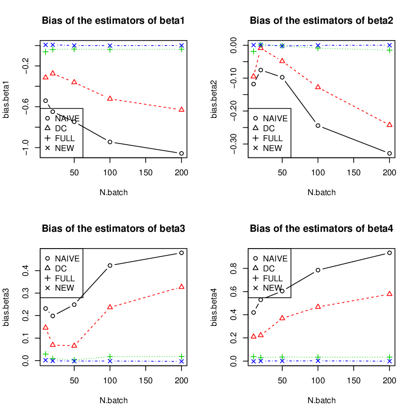
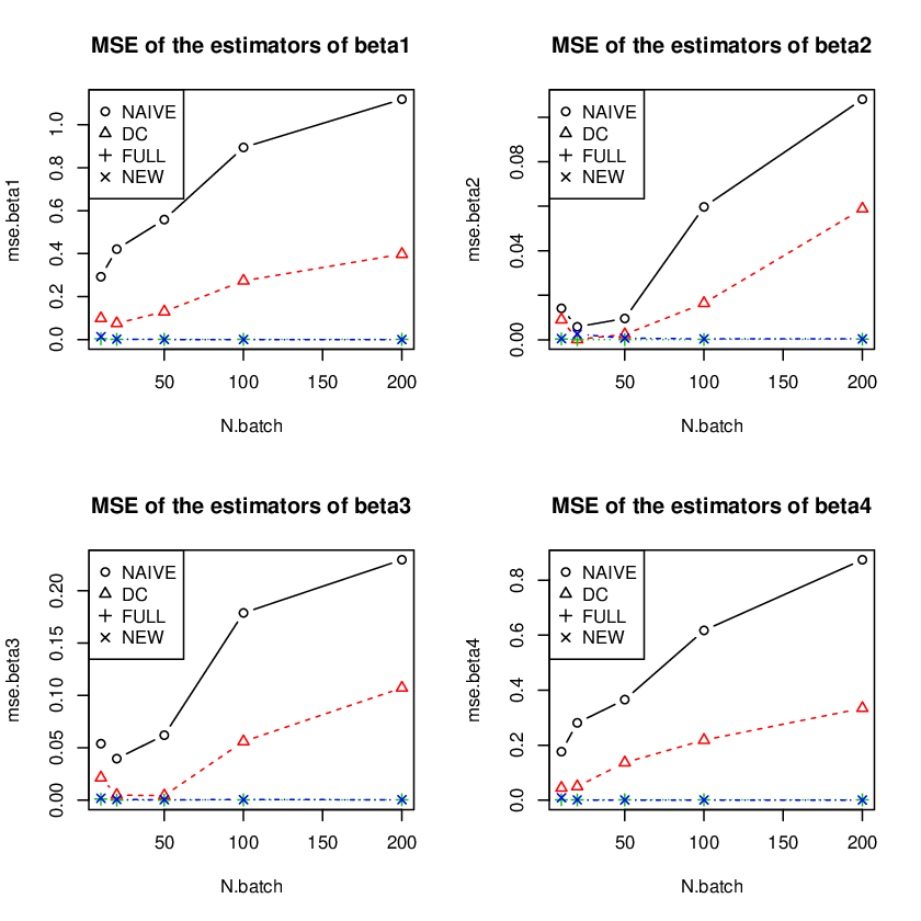
(Figure 1 and Figure 2 about here)
Figure 1 shows the empirical bias of all the estimators considered, and Figure 2 presents the estimated mean square error of the involved estimators. We have the following findings:
- 1)
The newly proposed BC-GE performs comparably well with the full data estimator. Actually, the difference between the BC-GE and full data estimator is negligible, and the bias and mean square error of both estimators are nearly zero for any choices of .
- 2)
Under criteria of estimation bias and mean square error, the BC-GE is much better than the naive averaging estimator and the DC-expression estimator uniformly for any choices of . Furthermore, the bias and mean square error of the naive averaging estimator and DC-expression estimator are increasing with the number , and both estimators are almost collapsed when is large.
- 3)
The naive averaging estimator is the worst one among the estimators considered for any choices of .
Experiment 2. Ridge-based estimators. Here we examine the behavior of the BC-GE for the Ridge estimation. For the linear regression model, the regression coefficients are chosen as , a 4-dimensional vector, and the covariance matrix of the covariate vector is chosen as with . The other experiment conditions are designed as the same as those in Experiment 1. Because this is non-sparse and low dimensional regression, and the correlation among the components of is relatively strong, we can use the Ridge estimation method to estimate .
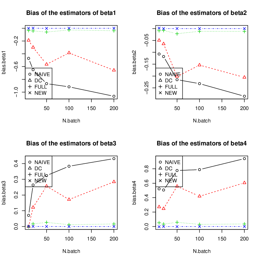
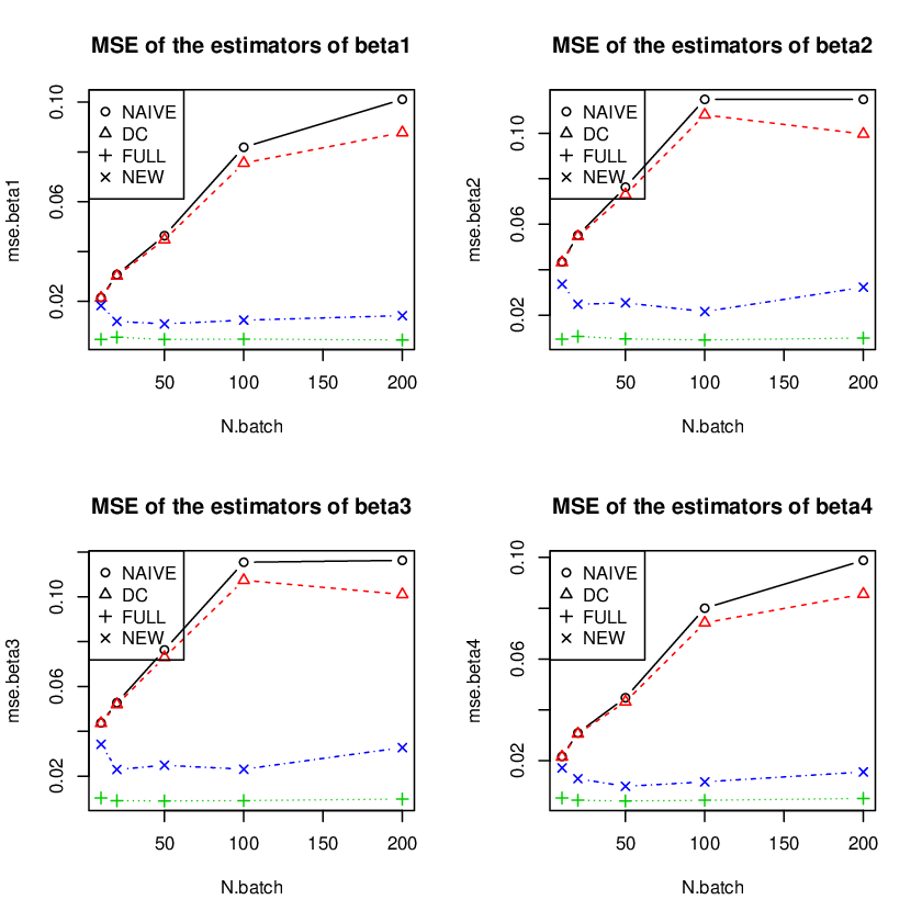
(Figure 3 and Figure 4 about here)
Figure 3 and Figure 4 report the empirical bias and mean square error of all the estimators. It can be seen that the fashions of the simulation results in Figure 3 and Figure 4 are the almost same as those in Figure 1 and Figure 2 of Experiment 1. In brief, the BC-GE is the best one, the naive averaging estimator is the worst one among all the estimators for any choices of , and particularly, when is large, the BC-GE is significantly better than the naive averaging estimator and the DC-expression estimator.
5.2 Linear model with identically distributed data
Experiment 3. LASSO-based estimators. The model settings are the same with those in Experiment 1, except for that the predictors in each batch are all generated from distribution , i.e., the only difference between this experiment and Experiment 1 is that the data in this experiment are homogeneously distributed, but the data in Experiment 1 are heterogeneously distributed. To guarantee the Condition C2, data and in batch are both multiplied by matrix , where , , are generated from normal distribution , .
(Figure 5 and Figure 6 about here)
Figure 5 and Figure 6 present the bias and mean square error of all the estimators. Similar to the case of identically distributed data, the BC-GE is the best one among all the estimators for any choices of , which has the similar behavior to that of the full data estimator. Particularly, when is large, the BC-GE is significantly better than the naive averaging estimator and the DC-expression estimator.
Experiment 4. Ridge-based estimators. The model settings are the same as those in Experiment 2, except for that the data in each batch are all generated from a common population, , and the regression coefficients are set as . To guarantee the Condition C2, the similar strategies as in Experiment 3 are employed to generate heterogenous data. The GCV criterion is employed to choose the penalty parameters .
(Figure 7 and Figure 8 about here)
Figure 7 and Figure 8 show the bias and mean square error of all the estimators. As can be seen from the figures, the proposed global estimator performs comparably well with the estimator based on the full data, moreover, it behaves significantly well in bias reduction for the ridge estimator, while the naive estimator performs worst among the four estimators.
5.3 Nonparametric model
Finally, we briefly examine the behavior of the new method in nonparametric model, although in the case the method has not been completely clarified and the related theoretical property has not been investigated aforementioned in Section 4.
Experiment 5. N-W-based estimators. Consider the following nonparametric regression
where , the errors are chosen as , the regression function is designed as and the sample size takes value 10000. The entire dataset are divided into batches with equal size .
In this experiment, the Gaussian kernel is employed to construct kernel estimators, and cross-validation is applied to select bandwidth . The simulation results are reported in Table 1, where the MISE stands for the empirical mean integrated squared error through repetitions. Moreover, the quantile curves of the BC-GE, naive averaging estimator and full data estimator for are also presented. Because the results are similar for different choices of batch , we only show the quantile curves for in Figure 9. Each subfigure contains , , and quantile curves of the nonparametric estimator and the true curve of .
| Num. of Batch () | BC-GE | Full data | Naive |
|---|---|---|---|
| 10 | 2.6179 (0.7112) | 3.7971 (1.6750) | 4.8143 (2.1532) |
| 20 | 2.9145 (0.7443) | 3.7924 (1.6744) | 4.8426 (2.1948) |
| 50 | 3.4878 (0.8774) | 3.8146 (1.7171) | 5.1255 (2.3524) |
| 100 | 5.8981 (1.3130) | 3.6669 (1.6132) | 6.9162 (2.9409) |
| 200 | 6.5604 (1.6244) | 3.6085 (1.5526) | 7.4841 (3.0450) |
Note: MISE and its standard deviation(in parenthesis) is in the scale of
(Figures 9 about here)
By comparing the MISEs and the quantile curves of the three estimators in Table 1 and Figures 9, respectively, we have the following findings: (1) Usually, the BC-GE estimator works well with small MISE compared with the full data and naive estimators; (2) The naive estimator performs worst among these estimators. Unlike the case of linear model, however, the number of batch clearly affects the performance of the BC-GE and naive averaging estimator. Note our method is based on (4.6) and (4.7), the estimating equation is not robust in the sense of Bontemps (2018). Thus, new technique (e.g., robust estimation equation method) should be developed in the future to improve the new method.
6 Conclusions and future works
In this paper, we established a global bias-correction divide-and-conquer framework for biased estimation under the case of big data. Our method for composition is based on a closed representation of the local estimators obtained by the data in each batch. Thus, the main difference from the classical DC method is that the new GBC-DC method can absorb the information hidden in the statistical structure and the variables in each batch of data. By such a representation and least squares, the resulting global estimator is strictly unbiased even if the local estimators have a non-negligible bias. On the other hand, the new method is simple and computationally efficient, without use of any iterative algorithm and local bias-correction. The theoretical properties show that new method behaves as the full data estimator for any choice of the number of batches. Moreover, our comprehensive simulation studies illustrate that the proposed GBC-DC approach is significantly bias-corrected, and the behavior is comparable with the full data estimation and is much better than the competitors.
Although we mainly fucus on linear model, our method can be extended into other models such as nonlinear and nonparametric regression models. However, some new techniques should be developed for these extensions. It is because the related representation is unprecise and contains a plug-in estimator. As a result, the theoretical property is difficult to be established and the finite sample behavior is not better than these in linear model. These are interesting issues and are worth further study in the future.
References
-
Battey, H., Fan, J., Liu, H., Lu, J. and Zhu, Z. (2018). Distributed testing and estimation under sparse high dimensional models. Ann. Statist., 46, 1352-1382.
-
Bhattacharya, P. K. and Gangopadhyay, A. (1990). Kernel and nearest neighbor estimation of a conditional quantile. Ann. Statist., 18, 1400-1415.
-
Bontemps, C. (2018). Moment-based tests under parameter uncertainty. Review of Economics and Statistics (To appear).
-
Bradic, J., Fan, J. and Wang, W. (2011). Penalized composite quasi-likelihood for ultrahigh dimensional variable selection. J. R. Statist. Soc., B, 73, 325-349.
-
Chaudhuri, P. (1991). Nonparametric estimates of regression quantiles and their local Bahadur representation. Ann. Statist., 19, 760-777.
-
Chen, X., Liu, W. and Zhang, Y. (2018). Quantile regression under memory constraint. Ann. Statist. To appear.
-
Chen, X. and Xie, M. (2014). A split-and-conquer approach for analysis of extraordinarily large data. Statist. Sinica, 1655-1684.
-
Chen, Y. X., Dong, G. Z., Han, J. W., Pei, J., Wah, B. W. and Wang, J. Y. (2006). Regression cubes with lossless compression and aggregation. IEEE Transaction on Knowledge and Data Engineering, 18, No. 12, 1-14.
-
Cheng, M. Y., Huang, T, Liu, P. and and Peng, H. (2018). Bias reduction for nonparametric and semiparametric regression models. Statistica Sinica, 28, 2749-2770.
-
Dai, W. L., Tong, T. J. and Zhu, L. X (2017), On the choice of difference sequence in a unified framework for variance estimation in nonparametric regression. Statistical Science, 32, 455-468.
-
Dai, W. L., Tong, T. J. and Genton, M. G. (2016), Optimal estimation of derivatives in nonparametric regression. Journal of Machine Learning Research, 17, 1¨C25.
-
Fan, J. and Wang, W. (2011). Penalized composite quasi-likelihood for ultrahigh dimensional variable selection. J. R. Statist. Soc. B, 73, 325-349.
-
Greenwald, M. B. and Khanna, S. (2004). Power-conserving computation of order statistics over sensor networks. In Proceedings of the ACM Symposium on Principles of Database Systems.
-
Guha, S. and Mcgregor, A. (2009). Stream order and order statistics: quantile estimation in random order streams. SIAM J. Comput., 38, 2044-2059.
-
He, X. M. and Shao, Q. M. (1996). A general Bahadur representation of -estimators and its application to linear regression with nonstochastic designs. Annals of Statistics, 24, 2608-2630.
-
Hong, S. Y. (2003). Bahadur representation and its applications for local polynomial estimation in nonparametric -regression. Nonparametric Statistics, 15, 237-251.
-
Jordan, M. I., Lee, J. D. and Yang, Y. (2018). Communication-efficient distributed statistical inference. J. Amer. Statist. Assoc. To appear.
-
Huang, J., Horowitz, J. L. and Ma, S. (2008). Asymptotic properties of Ridge estimation in spare high-dimensional regression models. Ann. Statist., 36, 578-613.
-
Jurečková, J. (1985). Representation of -estimators with the second-order asymptotic distribution. Statist. Decisions, 3, 263-276.
-
Jurečková J. and Sen, P. K. (1987). A second-order asymptotic distributional representation of -estimators with discontinuous score functions. Ann. Probab., 15 814-823.
-
Kai, B, Li, R. and Zou, H. (2010). Local composite quantile regression smoothing: an efficient and safe alterative to local polynomial regression. J. R. Statist. Soc. B, 72, 49-69.
-
Kai, B, Li, R. and Zou, H. (2011). New efficient estimation and variable selection methods for semiparametric varying-coefficient partially linear models. Ann. Statist., 39, 305-332.
-
Knight, K. and Fu, W. (2000). Asymptotics for Lasso-type estimators. Ann. Statist., 28, 1356-1378.
-
Lee, J. D., Liu, Q., Sun, Y. and Taylor, J. E. (2017). Communication-efficient sparse regression. J. Mach. Learn. Res., 18, 1-30.
-
Li, R., Lin, D. K. and Li, B. (2013). Statistical inference in massive data sets. Appl. Stoch. Model Bus. 29, 399-409.
-
Li, K. and Yang, J. (2018). Score-Matching Representative Approach for Big Data Analysis with Generalized Linear Models. Available via http://arxiv.org/ abs/1811.00462?context=stat.
-
Lian, H., Zhao, K. and Lv, S. G. (2018). Projected spline estimation of the nonparametric function in high-dimensional partially linear models for massive data. Ann. Statist. (To appear).
-
Lin, L. and Li, F. (2008). Stable and bias-corrected estimation for nonparametric regression models. Journal of Nonparametric Statistics, 20, 283-303.
-
Lin, L., Li, F., Wang, K. N. and Zhu, L. X. (2019). Composite estimation: An asymptotically weighted least squares approach. Statistica Sinica 29, 1367-1393.
-
Lin, N. and Xi, R. (2011). Aggregated Estimating Equation Estimation. Statistics and Its Interface, 4, 73-83.
-
Manku, G. S., Rajagopalan, S. and Lindsay, B. G. (1998). Approximate medians and other quantiles in one pass and with limited memory. In Proceedings of the ACM SIGMOD International Conference on Management of Data.
-
Mcdonald, R., Mohri, M., Silberman, N., Walker, D. and Mann, G. S. (2009). Efficient large-scale distributed training of conditional maximum entropy models. In Advances in Neural Information Processing Systems, 1231-1239.
-
Meinshausen, N. and Buhlmann, P. (2010). Stability selection. J. Roy. Statist. Soc. Ser., B 72, 417-473.
-
Jonathan, D. R., and Boaz, N. (2016). On the optimality of averaging in distributed statistical learning. Information and Inference: A Journal of the IMA, 5, 379-404.
-
Shah, R. and Samworth, R. J. (2013). Variable selection with error control: Another look at stability selection. J. Roy. Statist. Soc. Ser., B 75, 55-80.
-
Schifano, E. D., Wu, J., Wang, C., Yan, J., and Chen, M. H. (2016). Online updating of statistical inference in the big data setting. Technometrics, 58 (3), 393-403.
-
Shi, C., Lu, W. and Song, R. (2017). A massive data framework for -estimators with cubic-rate. J. Amer. Statist. Assoc. To appear.
-
Sun, J., Gai, Y. J. and Lin, L. (2013). Weighted local linear composite quantile estimation for the case of general error distributions. Journal of Statistical Planning and Inference, 143, 1049-1063.
-
Tibshirani, R. (1996). Regression shrinkage and selection via the lasso. Journal of the Royal Statistical Society, Series B, 58, 267-288.
-
Tong, T. and Wang, Y. (2005). Estimating residual variance in nonparametric regression using least squares. Biometrika, 92, 821-830.
-
van der Vaart, A. W. (1998). Asymptotic Statistics. Cambridge University Press.
-
Volgushev, S., Chao, S.-K. and Cheng, G. (2018). Distributed inference for quantile regression processes. Ann. Statist. To appear.
-
Wainwright, M. J. (2009). Sharp threshold for high-dimensional and noisy sparsity recovery using -constrained quadratic programming (Lasso). IEEE Transactions on Information Theory, 55, 2183-2202.
-
Wang, H., Yang, M. and Stufken, J. (2018) Information-based optimal subdata selection for big data linear regression. Journal of the American Statistical Association. To appear, available via https://haiying-wang.uconn.edu/wp-content/uploads/sites/2127/2017/04/IBOSS_Linear.pdf
-
Wang, J., Kolar, M., Srebro, N. and Zhang, T. (2017). Efficient distributed learning with sparsity. In Proceedings of the International Conference on Machine Learning.
-
Wang, W. W. and Lin, L. (2015). Derivative estimation based on difference sequence via locally weighted least squares regression. Journal of Machine Learning Research, 16, 2617-2641.
-
Wang. W. W., Yu, P., Lin, L. and Tong, T. J. (2019). Robust Estimation of Derivatives Using Locally Weighted Least Absolute Deviation Regression. Journal of Machine Learning Research, (to appear).
-
Zinkevich, M., Weimer, M., Li, L., and Smola, A. J. (2010). Parallelized stochastic gradient descent. In Advances in Neural Information Processing Systems, 2595-2603.
-
Zhang, Y., Duchi, J. and Wainwright, M. (2015). Divide and conquer kernel ridge regression: A distributed algorithm with minimax optimal rates. J. Mach. Learn. Res., 16, 3299-3340.
-
Zhang, Q. and Wang, W. (2007). A fast algorithm for approximate quantiles in high speed data streams. In Proceedings of the International Conference on Scientific and Statistical Database Management.
-
Zhang, Y., Duchi, J. C. and Wainwright, M. J. (2013). Communication-efficient algorithms for statistical optimization. Journal of Machine Learning Research, 14, 3321-3363.
-
Zhao, T., Cheng, G. and Liu, H. (2016). A partially linear framework for massive heterogeneous data. Ann. Statist., 44, 1400-1437.
-
Zou, H. and Yuan, M. (2008). Composite quantile regression and the oracle model selection theory. Ann. Statist., 36, 1108-1126.





Appendix: Proofs
Proof of Lemma 3.1. It is the direct result of the properties of expectation and variance of the original least squares estimation under linear model.
Proof of Lemma 3.2. By the formula for the block matrix inversion, we have
where . It follows from the definition of that
The results above, Lemma 3.1 and Condition C1 together imply that , and . These result in , and . Consequently, and Therefore, we have . The proof is completed.
Proof of Theorem 3.3. It is a direct result of Lemma 3.2.
Proof of Theorem 3.4. By the definition of the estimator, we have
where . This shows that has mean zero and covariance , and is normally distributed, asymptotically. Thus, we only need to calculate the asymptotic variance of .
The proof of Lemma 3.2 and Condition C3 indicate that
and moreover,
The proof is completed.