OSU-HEP-19-03
Minimal Dirac Neutrino Mass Models from Gauge
Symmetry and Left-Right Asymmetry at Colliders
Sudip Jana** * E-mail: sudip.jana@okstate.edu, Vishnu P.K.†† † E-mail: vipadma@okstate.edu and Shaikh Saad‡‡ ‡ E-mail: shaikh.saad@okstate.edu
Department of Physics, Oklahoma State University, Stillwater, OK 74078, USA
Abstract
In this work, we propose minimal realizations for generating Dirac neutrino masses in the context of a right-handed abelian gauge extension of the Standard Model. Utilizing only symmetry, we address and analyze the possibilities of Dirac neutrino mass generation via (a) tree-level seesaw and (b) radiative correction at the one-loop level. One of the presented radiative models implements the attractive scotogenic model that links neutrino mass with Dark Matter (DM), where the stability of the DM is guaranteed from a residual discrete symmetry emerging from . Since only the right-handed fermions carry non-zero charges under the , this framework leads to sizable and distinctive Left-Right asymmetry as well as Forward-Backward asymmetry discriminating from models and can be tested at the colliders. We analyze the current experimental bounds and present the discovery reach limits for the new heavy gauge boson at the LHC and ILC. Furthermore, we also study the associated charged lepton flavor violating processes, dark matter phenomenology and cosmological constraints of these models.
1 Introduction
Neutrino oscillation data [1] indicates that at-least two neutrinos have tiny masses. The origin of the neutrino mass is one of the unsolved mysteries in Particle Physics. The minimal way to obtain the non-zero neutrino masses is to introduce three right-handed neutrinos that are singlets under the Standard Model (SM). Consequently, Dirac neutrino mass term at the tree-level is allowed and has the form: . However, this leads to unnaturally small Yukawa couplings for neutrinos (). There have been many proposals to naturally induce neutrino mass mostly by using the seesaw mechanism [2, 3, 4, 5, 6] or via radiative mechanism [7]. Most of the models of neutrino mass generation assume that the neutrinos are Majorana 11 1 For a recent review on models based on Majorana neutrinos see Ref. [8]. For Majorana neutrino mass models within the context of simple grand unified theories see Ref. [9]. type in nature. Whether neutrinos are Dirac or Majorana type particles is still an open question. This issue can be resolved by neutrinoless double beta decay experiments [10]. However, up-to-now there is no concluding evidence from these experiments.
Recently, there has been a growing interest in models where neutrinos are assumed to be Dirac particles. Many of these models use ad hoc discrete symmetries [11, 12, 13, 14, 16, 17, 18, 15, 19, 20, 21] to forbid the aforementioned unnaturally small tree-level Yukawa term as well as Majorana mass terms. However, it is more appealing to forbid all these unwanted terms utilizing simple gauge extension of the SM instead of imposing discrete or continuous global symmetries. This choice is motivated by the fact that contrary to gauge symmetries, global symmetries are known not to be respected by the gravitational interactions [22, 23, 24, 25, 26].
In this work, we extend the SM with gauge symmetry, under which only the SM right-handed fermions are charged and the left-handed fermions transform trivially. This realization is very simple in nature and has several compelling features to be discussed in great details. Introducing only the three right-handed neutrinos all the gauge anomalies can be canceled and symmetry can be utilized to forbid all the unwanted terms to build desired models of Dirac neutrino mass. Within this framework, by employing the symmetry we construct a tree-level Dirac seesaw model [27] and two models where neutrino mass appears at the one-loop level. One of these loop models presented in this work is the most minimal model of radiative Dirac neutrino mass [28] and the second model uses the scotogenic mechanism [29] that links two seemingly uncorrelated phenomena: neutrino mass with Dark Matter (DM). As we will discuss, the stability of the DM in the latter scenario is a consequence of a residual discrete symmetry that emerges from the spontaneous breaking of the gauge symmetry.
Among other simple possibilities, one can also extend the SM with gauge symmetry [30] for generating the Dirac neutrino mass [31, 32, 33, 34, 28, 35]. Both of the two possibilities are attractive and can be regarded as the minimal gauge extensions of the SM. However, the phenomenology of model is very distinctive compared to the case. In the literature, gauged symmetry has been extensively studied whereas gauged extension has received very little attention.
Unlike the case, in our set-up, the SM Higgs doublet is charged under this symmetry to allow the desired Yukawa interactions to generate mass for the charged fermions, this leads to interactions with the new gauge boson that is absent in model. The running of the Higgs quartic coupling gets modified due to having such interactions with the new gauge boson that can make the Higgs vacuum stable [36]. Due to the same reason, the SM Higgs phenomenology also gets altered [37].
We show by detail analysis that despite their abelian nature, and have distinguishable phenomenology. The primary reason that leads to different features is: gauge boson couples only to the right-handed chiral fermions, whereas is chirality-universal. As a consequence, model leads to large left-right (LR) asymmetry and also forward-backward (FB) asymmetry that can be tested in the current and future colliders that make use of the polarized initial states, such as in ILC. We also comment on the differences of our scenario with the other models existing in the literature. Slightly different features emerge as a result of different charge assignment of the right-handed neutrinos in our set-up for the realization of Dirac neutrino mass. In the existing models, flavor universal charge assignment for the right-handed neutrinos are considered and neutrinos are assumed to be Majorana particles. Whereas, in our set-up, neutrinos are Dirac particles that demands non-universal charge assignment for the right-handed neutrinos under . Neutrinos being Dirac in nature also leads to null neutrinoless double beta decay signal.
The originality of this work is, by employing only the gauged symmetry, we construct Dirac neutrino masses at the tree-level and one-loop level (with or without DM) which has not been done before and, by a detailed study of the phenomenology associated to the new heavy gauge boson, we show that model is very promising to be discovered in the future colliders. Due to the presence of the TeV or sub-TeV scale BSM particles, these models can give rise to sizable rate for the charged lepton flavor violating processes which we also analyze. On top of that, we bring both the dark matter and the neutrino mass generation issues under one umbrella without imposing any additional symmetry and, work out the associated dark matter phenomenology. We also discuss the cosmological consequences due to the presence of the light right-handed neutrinos in our framework.
The paper is organized as follows. In Section 2, we discuss the framework where SM is extended by an abelian gauge symmetry . In Section 3, we present the minimal Dirac neutrino mass models in details, along with the particle spectrum and charge assignments. In Section 4, we discuss the running of the coupling. Charged lepton flavor violating processes are analyzed in Section 5. We have also done the associated dark matter phenomenology in Section 6 for the scotogenic model. Furthermore, we analyze the collider implications in Section 7. In Section 8, we study the constraints from cosmological measurement and finally, we conclude in Section 9.
2 Framework
Our framework is a very simple extension of the SM: an abelian gauge extension under which only the right-handed fermions are charged. Such a charge assignment is anomalous, however, all the gauge anomalies can be canceled by the minimal extension of the SM with just three right-handed neutrinos. Within this framework the minimal choice to generate the charged fermion masses is to utilize the already existing SM Higgs doublet, hence the associated Yukawa couplings have the form:
| (2.1) |
As a result, the choice of the charges of the right-handed fermions of the SM must be universal and obey the following relationship:
| (2.2) |
Here represents the charge of the particle . Hence, all the charges are determined once is fixed, which can take any value. The anomaly is canceled by the presence of the right-handed neutrinos that in general can carry non-universal charge under . Under the symmetry of the theory, the quantum numbers of all the particles are shown in Table I.
| Multiplets | |
|---|---|
| Quarks | |
| Leptons | |
| Higgs |
In our set-up, all the anomalies automatically cancel except for the following two:
| (2.3) | ||||
| (2.4) |
This system has two different types of solutions. The simplest solution corresponds to the case of flavor universal charge assignment that demands: which has been studied in the literature [38, 39, 40, 41, 42]. In this work, we adopt the alternative choice of flavor non-universal solution and show that the predictions and phenomenology of this set-up can be very different from the flavor universal scenario. We compare our model with the other extensions, as well as extensions of the SM. As already pointed out, a different charge assignment leads to distinct phenomenology in our model and can be distinguished in the neutrino and collider experiments.
Since SM is a good symmetry at the low energies, symmetry needs to be broken around TeV scale or above. We assume that gets broken spontaneously by the VEV of a SM singlet that must carry non-zero charge () under . As a result of this symmetry breaking, the imaginary part of will be eaten up by the corresponding gauge boson to become massive. Since EW symmetry also needs to break down around the GeV scale, one can compute the masses of the gauge bosons from the covariant derivatives associated with the SM Higgs and the SM singlet scalar :
| (2.5) | ||||
| (2.6) |
As a consequence of the symmetry breaking, the neutral components of the gauge bosons will all mix with each other. Inserting the following VEVs:
| (2.7) |
one can compute the neutral gauge boson masses as:
| (2.8) |
Where, and the well-known relation and furthermore GeV. In the above mass matrix denoted by , one of the gauge bosons remains massless, which must be identified as the photon field, . Moreover, two massive states appear which are the SM -boson and a heavy -boson (). The corresponding masses are given by:
| (2.9) |
here we define:
| (2.10) | ||||
| (2.11) |
Which clearly shows that for , the mass of the SM gauge boson is reproduced: . To find the corresponding eigenstates, we diagonalize the mass matrix as: , with:
| (2.12) |
From Eq. (2.9) one can see that the mass of the SM -boson gets modified as a consequence of gauge extension. Precision measurement of the SM -boson puts bound on the scale of the new physics. From the experimental measurements, the bound on the lower limit of the new physics scale can be found by imposing the constraint MeV [43]. For our case, this bound can be translated into:
| (2.13) |
With GeV [43], we find . Which corresponds to TeV for and (this charge assignment for the SM Higgs doublet and the SM singlet scalar that breaks will be used in Secs. 3 and 7).
Furthermore, the coupling of all the fermions with the new gauge boson can be computed from the following relevant part of the Lagrangian:
| (2.14) |
The couplings of all the fermions in our theory are collected in Table II and will be useful for our phenomenological study performed later in the text. Note that the couplings of the left-handed SM fermions are largely suppressed compared to the right-handed ones, since they are always proportional to and must be small and is highly constrained by the experimental data.
| Fermion, | Coupling, |
|---|---|
| Quarks | |
| Leptons | |
| Vector-like fermions |
Based on the framework introduced in this section, we construct various minimal models of Dirac neutrino masses in Sec 3 and study various phenomenology in the subsequent sections.
3 Dirac Neutrino Mass Models
By adopting the set-up as discussed above in this section, we construct models of Dirac neutrino masses. Within this set-up, if the solution is chosen which is allowed by the anomaly cancellation conditions, then tree-level Dirac mass term is allowed and observed oscillation data requires tiny Yukawa couplings of order . This is expected not to be a natural scenario, hence due to aesthetic reason we generate naturally small Dirac neutrino mass by exploiting the already existing symmetries in the theory. This requires the implementation of the flavor non-universal solution of the anomaly cancellation conditions, in such a scenario symmetry plays the vital role in forbidding the direct Dirac mass term and also all Majorana mass terms for the neutrinos.
In this section, we explore three different models within our framework where neutrinos receive naturally small Dirac mass either at the tree-level or at the one-loop level. Furthermore, we also show that the stability of DM can be assured by a residual discrete symmetry resulting from the spontaneous symmetry breaking of . In the literature, utilizing symmetry, two-loop Majorana neutrino mass is constructed with the imposition of an additional symmetry in [38, 39] and three types of seesaw cases are discussed, standard type-I seesaw in [40], type-II seesaw in [41] and inverse seesaw model in [42]. In constructing the inverse seesaw model, in addition to , additional flavor dependent U(1) symmetries are also imposed in [42]. In all these models, neutrinos are assumed to be Majorana particles which is not the case in our scenario.
3.1 Tree-level Dirac Seesaw
In this sub-section, we focus on the tree-level neutrino mass generation via Dirac seesaw mechanism [27]22 2 For correlating Dirac seesaw with leptogenesis, see for example [99, 100].. For the realization of this scenario, we introduce three generations of vector-like fermions that are singlets under the SM: . In this model, the quantum numbers of the multiplets are shown in Table III and the corresponding Feynman diagram for neutrino mass generation is shown in Fig. 1. This choice of the particle content allows one to write the following Yukawa coupling terms relevant for neutrino mass generation:
| (3.15) |
Here, we have suppressed the generation and the group indices. And the Higgs potential is given by:
| (3.16) |
When both the and EW symmetries are broken, the part of the above Lagrangian responsible for neutrino mass generation can be written as:
| (3.17) |
Where is a matrix and, since carries a different charge we have . The bare mass term of the vector-like fermions can in principle be large compared to the two VEVs, , assuming this scenario the light neutrino masses are given by:
| (3.18) |
Assuming TeV, , to get eV one requires GeV. Dirac neutrino mass generation of this type from a generic point of view without specifying the underline symmetry is discussed in [17].
| Multiplets | |
|---|---|
| Leptons | |
| Scalars | |
| Vector-like fermion |
 |
In this scenario two chiral massless states appear, one of them is , which is a consequence of its charge being different from the other two generations. In principle, all three generations of neutrinos can be given Dirac mass if the model is extended by a second SM singlet . When this field acquires an induced VEV all neutrinos become massive. This new SM singlet scalar, if introduced, gets an induced VEV from a cubic coupling of the form: . Alternatively, without specifying the ultraviolet completion of the model, a small Dirac neutrino mass for the massless chiral states can be generated via the dimension-5 operator once is broken spontaneously.
3.2 Simplest one-loop implementation
In this sub-section, we consider the most minimal [28] model of radiative Dirac neutrino mass in the context of symmetry. Unlike the previous sub-section, we do not introduce any vector-like fermions, hence neutrino mass does not appear at the tree-level. All tree-level Dirac and Majorana neutrino mass terms are automatically forbidden due to symmetry reasons. This model consists of two singly charged scalars to complete the loop-diagram and a neutral scalar to break the symmetry, the particle content with their quantum numbers is presented in Table IV.
| Multiplets | |
|---|---|
| Leptons | |
| Scalars |
With this particle content, the gauge invariant terms in the Yukawa sector responsible for generating neutrino mass are given by:
| (3.19) |
And the complete Higgs potential is given by:
| (3.20) |
By making use of the existing cubic term one can draw the desired one-loop Feynman diagram that is presented in Fig. 2. The neutrino mass matrix in this model is given by:
| (3.21) |
Here represents the mixing between the singly charged scalars and represents the mass of the physical state . Here we make a crude estimation of the neutrino masses: for radian, and one gets the correct order of neutrino mass eV.
 |
This is the most minimal radiative Dirac neutrino mass mechanism which was constructed by employing a symmetry in [44] and just recently in [33, 28] by utilizing symmetry. As a result of the anti-symmetric property of the Yukawa couplings , one pair of chiral states remains massless to all orders, higher dimensional operators cannot induce mass to all the neutrinos. As already pointed out, neutrino oscillation data is not in conflict with one massless state.
3.3 Scotogenic Dirac neutrino mass
The third possibility of Dirac neutrino mass generation that we discuss in this sub-section contains a DM candidate. The model we present here belongs to the radiative scotogenic [29] class of models and contains a second Higgs doublet in addition to two SM singlets. Furthermore, a vector-like fermion singlet under the SM is required to complete the one-loop diagram. The particle content of this model is listed in Table V and the associated loop-diagram is presented in Fig. 3.
| Multiplets | |
|---|---|
| Leptons | |
| Scalars | |
| Vector-like fermion |
 |
The relevant Yukawa interactions are given as follows:
| (3.22) |
And the complete Higgs potential is given by:
| (3.23) |
The SM singlet and the second Higgs doublet do not acquire any VEV and the loop-diagram is completed by making use of the quartic coupling . Here for simplicity, we assume that the SM Higgs does not mix with the other CP-even states, consequently, the mixing between and originates from the quartic coupling (and similarly for the CP-odd states). Then the neutrino mass matrix is given by:
| (3.24) | ||||
| (3.25) |
Where the mixing angle ( ) between the CP-even (CP-odd) states are given by:
| (3.26) |
For a rough estimation we assume no cancellation among different terms occurs. Then by setting TeV, TeV, , TeV, one can get the correct order of neutrino mass eV.
Since carries a charge of , a pair of chiral states associated with this state remains massless. However, in this scotogenic version, unlike the simplest one-loop model presented in the previous sub-section, all the neutrinos can be given mass by extending the model further. Here just for completeness, we discuss a straightforward extension, even though this is not required since one massless neutrino is not in conflict with the experimental data. If the model defined by Table V is extended by two SM singlets and a , all the neutrinos will get non-zero mass. The VEV of the field can be induced by the allowed cubic term of the form whereas, does not get any induced VEV.
Here we comment on the DM candidate present in this model. As aforementioned, we do not introduce new symmetries by hand to stabilize the DM. In search of finding the unbroken symmetry, first, we rescale all the charges of the particles in the theory given in Table V including the quark fields in such a way that the magnitude of the minimum charge is unity. From this rescaling, it is obvious that when the symmetry is broken spontaneously by the VEV of the field that carries six units of rescaled charge leads to: . However, since the SM Higgs doublet carries a charge of two units under this surviving symmetry, its VEV further breaks this symmetry down to: . This unbroken discrete symmetry can stabilize the DM particle in our theory. Under this residual symmetry, all the SM particles are even, whereas only the scalars and vector-like fermions are odd and can be the DM candidate. Phenomenology associated with the DM matter in this scotogenic model will be discussed in Sec. 6.
4 Running of the Gauge Coupling
In this section, we briefly discuss the running of the gauge coupling , at the one-loop level in our framework. The associated -function can be written as:
| (4.27) |
Where the coefficient can be calculated from [45]:
| (4.28) |
The first (second) sum is over the fermions (scalars), (). Here, for Weyl fermions, is the number of fermion generations, for complex scalars and are the Dynkin indices of the representations with the appropriate multiplicity factors. By solving Eq. (4.27), the Landau pole can be found straightforwardly:
| (4.29) |
The scale of the Landau pole depends on the value of the coupling , at the input scale . Depending on the choice, both the and scenarios can emerge.
Utilizing the basic set-up defined in Sec. 2, we have constructed three different models in Sec. 3, which correspond to three different coefficients for the Dirac seesaw, simplest one-loop, and Scotogenic models respectively. For demonstration purpose, we choose TeV and show the scale as a function of gauge coupling in Fig. 4 for the three different models discussed in this work. As expected, the higher the value of , smaller the gets.
5 Lepton Flavor Violation
In this section, we pay special attention to the charged lepton flavor violation (cLFV) which is an integral feature of these Dirac neutrino mass models. These lepton flavor violating processes provide stringent constraints on TeV-scale extensions of the standard model and, as a consequence put restrictions on the free parameters of our theories. For the first model we discussed, where neutrino masses are generated via Dirac seesaw mechanism, the cLFV decay rates induced by the neutrino mixings (cf. Fig. 5) are highly suppressed by the requirement that the scale of new physics (vector-like fermions ) is at GeV to satisfy the neutrino oscillation data, with Yukawa couplings being order one, and hence, are well below the current experimental bounds. Here, we can safely ignore cLFV processes associated with Dirac seesaw model. On the other hand, in the simplest one-loop Dirac neutrino mass model and in the scotogenic model, several new contributions appear due to the additional contributions from charged scalars (cf. Fig. 5), which could lead to sizable cLFV rates.
   |
  |
 |
The cLFV decay processes arise from one-loop diagrams are shown in Fig. 5. Let us now focus on the major cLFV processes in the simplest one-loop Dirac neutrino mass model. Processes of these types are most dominantly mediated by both the singlet charged scalars (). However, the charged scalar determines the chirality of the initial and final-state charged leptons to be left-handed, whereas mediated process fixes the chirality to be right-handed and hence there will be no interference between these two contributions. The Yukawa term is anti-symmetric in nature, whereas has completely arbitrary elements in the second and third rows (recall the restriction ). We can always make such a judicious choice that no more than one entry in a given row of can be large and thus we can suppress the contribution from the charged scalar for the cLFV processes. The expression for decay rates can be expressed as33 3 The general expression for this decay rate can be found in Ref. [46, 47]. :
| (5.30) |
  |
 |
In Fig. 6, we have shown the contour plots for branching ratio predictions for the cLFV processes: (top left), (top right) and (bottom) as a function of mass and Yukawa plane in simplest one-loop Dirac neutrino mass model. Red solid lines indicate the current bounds on branching ratios: 4.2 [48] for the (top left) process, 3.3 [49] for the (top right) process and 4.4 [49] for the (top right) process. Red dashed lines indicate the future projected bounds on the branching ratios: 6 [50] for the (top left), 3 [51] for the (top right) and 3 [51] for the (top right) processes respectively. For simplicity, we choose GeV. As we can see from the Fig. 6, is the most constraining cLFV process in this model. Since this could lead to sizable rates, it can be tested in the upcoming experiments.
Similarly, we analyze the major cLFV processes in scotogenic Dirac neutrino mass model. The representative Feynman diagram for the cLFV process is shown in Fig. 5 (right diagram). Here also, charged Higgs , which is the part of the doublet , mainly contributes to the cLFV process (cf. Fig. 5). The decay rate for solely depends on the two mass terms and Yukawa term . The decay width expression for this process can be written as:
| (5.31) |
Here, , and the function is expressed as [46, 47]
| (5.32) |
In Fig. 7, we have shown the branching ratio predictions for the different cLFV processes: (top left), (top right) and (bottom) as a function of mass in scotogenic one-loop Dirac neutrino mass model for three benchmark values of Yukawas: and . For our analysis, we set the vector-like fermion mass to be 5 TeV. The process imposes the most stringent bounds. In this set-up, for the Yukawas: and , we get charged Higgs mass bounds to be 3.1 TeV, 4.6 TeV and 5 TeV respectively. As we can see from Fig. 7, most of the parameter space in this model is well-consistent with these cLFV processes and which can be testable at the future experiments. We have shown the future projection reach for these cLFV processes by red dashed lines in Fig. 7.
6 Dark Matter Phenomenology
In this section, we briefly discuss the Dark Matter phenomenology in the scotogenic Dirac neutrino mass model. As aforementioned, in this model, a subgroup of the original symmetry remains unbroken that can stabilize the DM particle. Under this residual symmetry, all the SM particles are even, whereas only the scalars and vector-like Dirac fermion are odd and the lightest among these can be the DM candidate. DM phenomenology associated with the neutral component of inert scalar doublet, is extensively studied in Ref. [52] in a different set-up and corresponding study has been done for the neutral singlet scalar, in Ref. [53, 54]. In the following analysis, we consider to be the lightest among all of these particles, hence serves as a good candidate for DM (for simplicity we will drop the subscript from in the following). We aim to study the DM phenomenology associated with the vector-like Dirac fermion here. Due to Dirac nature of the dark matter, the phenomenology associated with it is very different from the Majorana fermionic dark matter scenario [55].
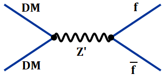 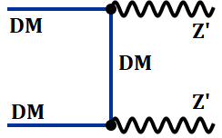 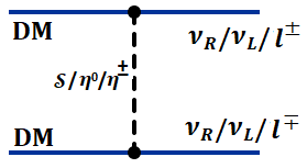 |
  |
In our case, pairs can annihilate through s-channel exchange process to a pair of SM fermions and right-handed neutrinos. Furthermore, if , then may also annihilate directly into pairs of on-shell bosons, which subsequently decay to SM fermions. It can also annihilate to SM fermions and right-handed neutrinos via channel scalar () exchanges. The representative Feynman diagrams for the annihilation of DM particle are shown in Fig. 8. It is important to mention that for the Majorana fermionic dark matter case, the annihilation rate is wave () suppressed since the vector coupling to a self-conjugate particle vanishes, on the contrary, the annihilation rate is not suppressed for the Dirac scenario (-wave). The non-relativistic form for this annihilation cross-section can be found here [58]. In Fig. 9, we analyze the dark matter relic abundance as a function of dark matter mass for various gauge couplings (left) and boson masses (right). Horizontal red and blue lines represent WMAP [56] relic density constraint and the PLANCK constraint [57] respectively. For simplicity, we set TeV (left) and provide the relic abundance prediction for two different values of gauge coupling (= 0.1 and 0.277). For the right plot in Fig. 9, DM relic abundance is analyzed for two different values of the masses and 20 TeV setting = 0.1. As expected, we can satisfy the WMAP [56] relic density constraint and the PLANCK constraint [57] for most of the parameter space in our model as long as is not too far away from mass. Throughout our DM analysis, we make sure that we are consistent with the SM boson mass correction constraint while choosing specific and values.
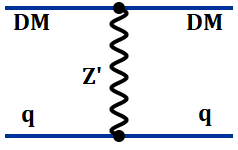 |

In addition to the relic density, we also take into account the constraints from DM direct detection experiments. In case of Majorana fermionic dark matter, at the tree-level, the spin-independent DM-nucleon scattering cross-section vanishes. However, at the loop-level, the spin-independent operators can be generated and hence it is considerably suppressed. The dominant direct detection signal remains the spin-dependent DM-nucleon scattering cross-section which for the Majorana fermionic dark matter is four times that for the Dirac-fermionic dark matter case. In general, the interactions induce both spin-independent (SI) and spin-dependent (SD) scattering with nuclei. The representative Feynman diagram for the DM-nucleon scattering is shown in Fig. 10. Particularly, in the scotogenic Dirac neutrino mass model, DM can interact with nucleon through channel exchange. Hence, large coherent spin-independent scattering may occur since both dark matter and the valence quarks of nucleons possess vector interactions with and this process is severely constrained by present direct detection experiment bounds. The DM-nucleon scattering cross-section is estimated in Ref. [58]. In Fig. 11, we analyze the spin-independent dark matter-nucleon scattering cross-section, (in pb) as a function of the dark matter mass with different gauge coupling . For this plot, we set TeV. Yellow, blue and green color solid lines represent current direct detection cross-section limits from LUX-2017 [59], XENON1T [60] and PandaX-II (2017) [61] experiments respectively. As can be seen from Fig. 11, we can satisfy all the present direct detection experiment bounds as long as we are consistent with the other severe bounds on mass and arising from colliders to be discussed in the next section.
7 Collider Implications
Models with extra implies a new neutral boson, which contains a plethora of phenomenological implications at colliders. Here we mainly focus on the phenomenology of the heavy gauge boson emerging from .
7.1 Constraint on Heavy Gauge Boson from LEP
There are two kinds of searches: indirect and direct. In case of indirect searches, one can look for deviations from the SM which might be associated with the existence of a new gauge boson . This generally involves precision EW measurements below and above the Z-pole. collision at LEP experiment [62] above the Z boson mass provides significant constraints on contact interactions involving and fermion pairs. One can integrate out the new physics and express its influence via higher-dimensional (generally dim-6) operators. For the process , contact interactions can be parameterized by an effective Lagrangian, , which is added to the SM Lagrangian and has the form:
| (7.33) |
Where is the new physics scale, is the Kronecker delta function, indicates all the fermions in the model and takes care of the chirality structure coefficients. The exchange of the new boson state emerging from can be stated in a similar way:
| (7.34) |
Due to the nature of gauge symmetry, the above interaction favors only the right-handed chirality structure. Thus, the constraint on the scale of the contact interaction for the process from LEP measurements [62] will indirectly impose bound on mass and the gauge coupling that can be translated into:
| (7.35) |
Other processes such as and impose somewhat weaker bounds than the ones quoted in Eq. 7.35.
7.2 Heavy Gauge Boson at the LHC
 |
Now we analyze the physics of the heavy neutral gauge boson at the Large Hadron Collider (LHC). At the LHC, can be resonantly produced via the quark fusion process since the coupling of with right-handed quarks () are not suppressed. After resonantly produced at the LHC, will decay into SM fermions and also to the exotic scalars () or fermions () depending on the model if kinematically allowed44 4 Even if we include decay modes, the branching fraction () for mode does not change much.. The present lack of any signal for di-lepton resonances at the LHC dictates the stringent bound on the mass and coupling constant in our model as the production cross-section solely depends on these two free parameters. Throughout our analysis, we consider that the mixing angle is not very sensitive (). In order to obtain the constraints on these parameter space, we use the dedicated search for new resonant high-mass phenomena in di-electron and di-muon final states using fb-1 of proton-proton collision data, collected at TeV by the ATLAS collaboration [63]. The searches for high mass phenomena in di-jet final states [64] will also impose bound on the model parameter space, but it is somewhat weaker than the di-lepton searches due to large QCD background. For our analysis, we implement our models in FeynRulesv2.0 package [65] and simulate the events for the process with MadGraph5aMC@NLOv301 code [66]. Then, using parton distribution function (PDF) NNPDF23loas0130 [67], the cross-section and cut efficiencies are estimated. Since no significant deviation from the SM prediction is observed in experimental searches [63] for high-mass phenomena in di-lepton final states, the upper limit on the cross-section is derived from the experimental analyses [63] using BR , where is the number of reconstructed heavy candidate, is the resonant production cross-section of the heavy , BR is the branching ratio of decaying into di-lepton final states , is the acceptance times efficiency of the cuts for the analysis. In Fig. 12, we have shown the upper limits on the cross-section at 95 C.L. for the process as a function of the di-lepton invariant mass using ATLAS results [63] at = 13 TeV with 36.1 fb-1 integrated luminosity. Red solid, dashed and dotted lines in Fig. 12 indicate the model predicted cross-section for three different values of gauge coupling constant respectively. We find that mass should be heavier55 5 For related works see also [68, 69]. than and TeV for three different values of gauge coupling constant and .
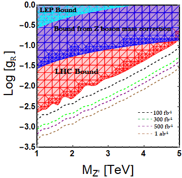 |
In Fig. 13, we have shown all the current experimental bounds in plane. Red meshed zone is excluded from the current experimental di-lepton searches [63]. The cyan meshed zone is forbidden from the LEP constraint[62] and the blue meshed zone is excluded from the limit on SM Z boson mass correction: TeV as aforementioned. We can see from Fig. 13 that the most stringent bound in plane is coming from direct searches at the LHC. After imposing all the current experimental bounds, we analyze the future discovery prospect of this heavy gauge boson within the allowed parameter space in plane looking at the prompt di-lepton resonance signature at the LHC. We find that a wider region of parameter space in plane can be tested at the future collider experiment. Black, green, purple and brown dashed lines represent the projected discovery reach at significance at 13 TeV LHC for 100 fb-1, 300 fb-1, 500 fb-1 and 1 ab-1 luminosities. On the top of that, the right-handed chirality structure of can be investigated at the LHC by measuring Forward-Backward (FB) and top polarization asymmetries in mode [70] and which can discriminate our interaction from the other interactions in model. The investigation of other exotic decay modes of heavy is beyond the scope of this article and shall be presented in a future work since these will lead to remarkable multi-lepton or displaced vertex signature [71, 72, 73, 74, 75, 76, 77] at the colliders.
7.3 Heavy Gauge Boson at the ILC
Due to the point-like structure of leptons and polarized initial and final state fermions, lepton colliders like ILC will provide much better precision of measurements. The purpose of the search at the ILC would be either to help identifying any discovered at the LHC or to extend the discovery reach (in an indirect fashion) following effective interaction. Even if the mass of the heavy gauge boson is too heavy to directly probe at the LHC, we will show that by measuring the process , the effective interaction dictated by Eq. 7.34 can be tested at the ILC. Furthermore, analysis with the polarized initial states at ILC can shed light on the chirality structure of the effective interaction and thus it can distinguish between the heavy gauge boson emerging from extended model and the from other extended model such as . The process typically exhibits asymmetries in the distributions of the final-state particles isolated by the angular- or polarization-dependence of the differential cross-section. These asymmetries can thus be utilized as a sensitive measurement of differences in interaction strength and to distinguish a small asymmetric signal at the lepton colliders. In the following, the asymmetries (Forward-Backward asymmetry, Left-Right asymmetry) related to this work will be described in great detail.
7.3.1 Forward-Backward Asymmetry
The differential cross-section in Eq. 7.3.1 is asymmetric in polar angle, leading to a difference of cross-sections for decays between the forward and backward hemispheres. Earlier, LEP experiment [62] used Forward-backward asymmetries to measure the difference in the interaction strength of the -boson between left-handed and right-handed fermions, which gives a precision measurement of the weak mixing angle. Here we will show that our framework leads to sizable and distinctive Forward-Backward (FB) asymmetry discriminating from other models and which can be tested at the ILC, since only the right-handed fermions carry non-zero charges under the . For earlier analysis of FB asymmetry in the context of other models as well as model-independent analysis see for example Refs. [78, 79, 80, 81, 82, 83, 84, 85, 86, 87, 88, 40, 42].
  |
At the ILC, effects have been studied for the following processes:
| (7.36) | ||||
| (7.37) | ||||
| (7.38) |
where are the helicities of initial (final)-state leptons and ’s are the momenta. Since the process is the most sensitive one at the ILC, we will focus on this process only for the rest of our analysis. One can write down the corresponding helicity amplitudes as:
| (7.39) | ||||
| (7.40) | ||||
| (7.41) | ||||
| (7.42) |
where , , and indicates the scattering polar angle. with QED coupling constant, and and is the weak mixing angle.
For a purely polarized initial state, the differential cross-section is expressed as:
| (7.43) |
Then the differential cross-section for the partially polarized initial state with a degree of polarization for the electron beam and for the positron beam can be written as [78, 40]:
| (7.44) |
One can now define polarized cross-section (for the realistic values at the ILC [89]) as:
| (7.45) | ||||
| (7.46) |
Using this one can study the initial state polarization-dependent forward-backward asymmetry as:
where
| (7.47) | ||||
| (7.48) |
where represents the integrated luminosity, indicates the efficiency of observing the events, and is a kinematical cut chosen to maximize the sensitivity. For our analysis we consider , and . Then we estimate the sensitivity to contribution by:
| (7.49) |
where and are FB asymmetry originated from both the SM and contribution and from the SM case only. Next, it is compared with the statistical error of the asymmetry (in only SM case) [78, 40]:
| (7.50) |
In Fig. 14, we analyze the strength of FB asymmetry as a function of VEV for both left and right-handed polarized cross-sections of the process. In order to compare, we have done the analysis for both the cases: from both and cases. We have considered the center of mass energy for the ILC at GeV and the integrated luminosity is set to be 1 ab-1 (5 ab-1) for the left (right) panel of Fig. 14. The grey shaded region corresponds to excluded region from the SM boson mass correction. Red dashed (solid) line represents for case for left (right) handed polarized cross-sections of the process, whereas blue dotted (dashed) line indicates for case for left (right) handed polarized cross-sections. From Fig. 14, we find that in case of model, it provides significant difference of for and due to the right-handed chirality structure of interaction from , while in the case of model, it provides small difference. Hence by comparing the difference of for differently polarized cross-section and at the ILC, we can easily discriminate the interaction from and model. As we can see from Fig. 14 that there are significant region for TeV which can give more than sensitivity for FB asymmetry by looking at process at the ILC. We can also expect much higher sensitivity while combining different final fermionic states such as other leptonic modes () as well as hadronic modes . Moreover, the sensitivity to interactions can be enhanced by analyzing the scattering angular distribution in details, although it is beyond the scope of our paper.
7.3.2 Left-Right Asymmetry
  |
The simplest example of the EW asymmetry for an experiment with a polarized electron beam is the left-right asymmetry , which measures the asymmetry at the initial vertex. Since there is no dependence on the final state fermion couplings, one can get an advantage by looking at LR asymmetry at lepton collider. Another advantage of this LR asymmetry measurement is that it is barely sensitive to the details of the detector. As long as at each value of , its detection efficiency of fermions is the same as that for anti-fermions, the efficiency effects should be canceled within the ratio because the decays into a back-to-back fermion-antifermion pair and about the midplane perpendicular to the beam axis, the detector was designed to be symmetric. For earlier studies on LR asymmetry in different contexts, one can see for example Refs. [78, 79, 80, 81, 82, 83, 84, 85, 86, 87, 88, 90]. LR asymmetry is defined as:
where is the number of events in which initial-state particle is left-polarized, while is the corresponding number of right-polarized events.
| (7.51) | ||||
| (7.52) |
Similarly, one can estimate the sensitivity to contribution in LR asymmetry by [79, 90, 82]:
| (7.53) |
with a statistical error of the asymmetry , given [79, 90, 82] as
| (7.54) |
 |
In Fig. 15, we analyze the strength of LR asymmetry for the process as a function of VEV . In order to distinguish interaction, we have analysed both the cases: emerging from both and cases. We have considered the center of mass energy for the ILC at GeV and the integrated luminosity is set to be 1 ab-1 (5 ab-1) for the left (right) panel of Fig. 15. The grey shaded region corresponds to excluded region from the SM boson mass correction. Red (blue) solid line represents for () case. From Fig. 15, we find that in case of model, it provides remarkably large LR asymmetry due to the right-handed chirality structure of interaction from , while in case of model, it gives a smaller contribution. Hence by comparing the difference of at the ILC, we can easily discriminate the interaction from and model. As we can see from Fig. 15 that there is a significant region for TeV which can give more than sensitivity for LR asymmetry by looking at process at the ILC. Even if, we can achieve sensitivity for a larger parameter space in our framework if integrated luminosity of ILC is upgraded to ab-1. Although, measurement of both the FB and LR asymmetries at the ILC can discriminate interaction for model from other extended models such as model, it is needless to mention that the LR asymmetry provides much better sensitivity than the FB asymmetry in our case. In Fig. 16, we have shown the survived parameter space in plane satisfying all existing bounds and which can be probed at the ILC in future by looking at LR asymmetry strength. Green and yellow shaded zones correspond to sensitivity confidence levels 1 and 2 by measuring LR asymmetry for extended model at the ILC. For higher mass (above 10 TeV), it is too heavy to directly produce and probe at the LHC looking at prompt di-lepton signature. On the other hand, ILC can probe the heavy effective interaction and LR asymmetry can pin down/distinguish our model from other existing extended model for a large region of the parameter space. Thus, search at the ILC would help to identify the origin of boson as well as to extend the discovery reach following effective interaction.
8 Constraint from Cosmology
In the previous section, we have extensively analyzed the collider implications of the new gauge boson . In this section, we aim to study the constraints on the mass of the new gauge boson from cosmological measurements and compare with the collider bounds. Since the right-handed neutrinos carry non-zero charge in our set-up, they couple to the SM sector via the boson interactions. Furthermore, since they are either massless or very light, they contribute to the relativistic degrees of freedom , hence in principle can increase the expansion rate of the Universe. Their contribution to this process is parametrized by and to compute it we follow the procedure discussed in Ref. [91]. After states decouple, specifically for ( represents the decoupling temperature of the neutrinos) their total contribution is given by:
| (8.55) |
here is the number of massless or light right-handed neutrinos, is the relativistic degrees of freedom at temperature T, with the well-known quantities and MeV [92]. For the following computation, we take the temperature-dependent degrees of freedom from the data listed in Table S2 of Ref. [93], and by utilizing the cubic spline interpolation method, we present as a function of in Fig. 17 (left plot).
The current cosmological measurement of this quantity is [94], which is completely consistent with the SM prediction [95]. These data limit the contribution of the right-handed neutrinos to be . However, future measurements [96] can put even tighter constraints on this deviation . The right-handed neutrinos decouple from the thermal bath when the interaction rate drops below the expansion rate of the Universe:
| (8.56) |
Here the Hubble expansion parameter is defined as:
| (8.57) |
where is the Planck mass and is the spin degrees of freedom of the right-handed neutrinos. And the interaction rate that keeps the right-handed neutrinos at the thermal bath is given by:
| (8.58) |
Here, the Fermi-Dirac distribution is , the number density is , and . Furthermore, the annihilation cross-section is as follows:
| (8.59) |
Where and represent the color degrees of freedom and the charge under the for a fermion respectively.

By plugging Eqs. (8.57)-(8.59) in Eq. (8.56) and then solving numerically, we present our result of as a function of in Fig. 17 (right plot). From this figure, one sees that cosmology provides strong bound on the mass of the new gauge boson based on the associated decoupling temperature of the right-handed neutrinos. The blue curve corresponds to the contribution of all the three right-handed neutrinos and the red dashed line represents the current experimental upper bound on the deviation of . This bound puts the restriction TeV, which is quite stronger than the LEP bound TeV, however, lies within the constraint provided by the SM -boson mass correction TeV. The framework presented in this work puts larger bound on the mass of the new gauge boson from cosmology due to large charge assignment of the right-handed neutrinos compared to the conventional models with universal charge, TeV [97, 98].
9 Conclusions
We believe that the scale of new physics is not far from the EW scale and a simple extension of the SM should be able to address a few of the unsolved problems of the SM. Adopting this belief, in this work, we have explored the possibility of one of the most minimal gauge extensions of the SM which is that is responsible for generating Dirac neutrino mass and may also stabilize the DM particle. Cancellations of the gauge anomalies are guaranteed by the presence of the right-handed neutrinos that pair up with the left-handed partners to form Dirac neutrinos. Furthermore, this symmetry is sufficient to forbid all the unwanted terms for constructing naturally light Dirac neutrino mass models without imposing any additional symmetries by hand. The chiral non-universal structure of our framework induces asymmetries, such as forward-backward asymmetry and especially left-right asymmetry that are very distinct compared to any other models. By performing detailed phenomenological studies of the associated gauge boson, we have derived the constraints on the model parameter space and analyzed the prospect of its testability at the collider such as at LHC and ILC. We have shown that a heavy (emerging from ), even if its mass is substantially higher than the center of mass energy available at the ILC, would manifest itself at tree-level by its propagator effects producing sizable contributions to the LR asymmetry or FB asymmetry. This can be taken as an initial guide to explore the model at colliders. These models can lead to large lepton flavor violating observables which we have studied and they could give a complementary test for these models. In this work, we have also analyzed the possibility of having a viable Dirac fermionic DM candidate stabilized by the residual discrete symmetry originating from , which connects to SM via portal coupling in a framework that also cater for neutrino mass generation. The DM phenomenology is shown to be crucially dictated by the interaction of with . Furthermore, we have inspected the constraints coming from the cosmological measurements and compared this result with the different collider bounds. For a comparison, here we provide a benchmark point by fixing the gauge coupling . With this, the current upper bound on the mass is TeV from 13 TeV LHC data with luminosity, and the future projection reach limit translates into TeV with luminosity. Whereas for the same value of the gauge coupling, the ILC has the discovery reach of TeV at the confidence level looking at the left-right asymmetry. The corresponding bounds from LEP, boson mass correction and from cosmology are TeV respectively, which are somewhat weaker compared to LHC and ILC bounds. To summarize, the presented Dirac neutrino mass models are well motivated and have rich phenomenology.
Acknowledgments
We thank K. S. Babu, Bhupal Dev and S. Nandi for useful discussions. The work of SJ and VPK was in part supported by US Department of Energy Grant Number DE-SC 0016013. The work of SJ was also supported in part by the Neutrino Theory Network Program. SJ thanks the Theoretical Physics Department at Washington University in St. Louis for warm hospitality during the completion of this work.
References
- [1] L. H. Whitehead [MINOS Collaboration], “Neutrino Oscillations with MINOS and MINOS+,” Nucl. Phys. B 908, 130 (2016) [arXiv:1601.05233 [hep-ex]]; M. P. Decowski [KamLAND Collaboration], “KamLAND’s precision neutrino oscillation measurements,” Nucl. Phys. B 908, 52 (2016); K. Abe et al. [T2K Collaboration], “Combined Analysis of Neutrino and Antineutrino Oscillations at T2K,” Phys. Rev. Lett. 118, no. 15, 151801 (2017) [arXiv:1701.00432 [hep-ex]]; P. F. de Salas, D. V. Forero, C. A. Ternes, M. Tortola and J. W. F. Valle, “Status of neutrino oscillations 2018: 3 hint for normal mass ordering and improved CP sensitivity,” Phys. Lett. B 782, 633 (2018) [arXiv:1708.01186 [hep-ph]].
- [2] P. Minkowski, Phys. Lett. B 67 (1977) 421; T. Yanagida, proceedings of the Workshop on Unified Theories and Baryon Number in the Universe, Tsukuba, 1979, eds. A. Sawada, A. Sugamoto; S. Glashow, in Cargese 1979, Proceedings, Quarks and Leptons (1979); M. Gell-Mann, P. Ramond, R. Slansky, proceedings of the Supergravity Stony Brook Workshop, New York, 1979, eds. P. Van Niewenhuizen, D. Freeman; R. Mohapatra, G. Senjanovic, “Neutrino Mass and Spontaneous Parity Violation,” Phys.Rev.Lett. 44 (1980) 912.
- [3] M. Magg and C. Wetterich, “Neutrino Mass Problem and Gauge Hierarchy,” Phys. Lett. B 94, 61 (1980); J. Schechter and J. W. F. Valle, “Neutrino Masses in SU(2) x U(1) Theories,” Phys. Rev. D 22, 2227 (1980); G. Lazarides, Q. Shafi and C. Wetterich, “Proton Lifetime and Fermion Masses in an SO(10) Model,” Nucl. Phys. B 181, 287 (1981); R. N. Mohapatra and G. Senjanovic, “Neutrino Masses and Mixings in Gauge Models with Spontaneous Parity Violation,” Phys. Rev. D 23, 165 (1981).
- [4] R. Foot, H. Lew, X. G. He and G. C. Joshi, “Seesaw Neutrino Masses Induced by a Triplet of Leptons,” Z. Phys. C 44, 441 (1989).
- [5] R. N. Mohapatra, “Mechanism for Understanding Small Neutrino Mass in Superstring Theories,” Phys. Rev. Lett. 56, 561 (1986); R. N. Mohapatra and J. W. F. Valle, “Neutrino Mass and Baryon Number Nonconservation in Superstring Models,” Phys. Rev. D 34, 1642 (1986).
- [6] E. Bertuzzo, S. Jana, P. A. N. Machado and R. Zukanovich Funchal, “Neutrino Masses and Mixings Dynamically Generated by a Light Dark Sector,” Phys. Lett. B 791, 210 (2019) [arXiv:1808.02500 [hep-ph]].
- [7] T. P. Cheng and L. F. Li, “On Weak Interaction Induced Neutrino Oscillations,” Phys. Rev. D 17, 2375 (1978); A. Zee, “A Theory of Lepton Number Violation, Neutrino Majorana Mass, and Oscillation,” Phys. Lett. 93B, 389 (1980) Erratum: [Phys. Lett. 95B, 461 (1980)]; T. P. Cheng and L. F. Li, “Neutrino Masses, Mixings and Oscillations in SU(2) x U(1) Models of Electroweak Interactions,” Phys. Rev. D 22, 2860 (1980); K. S. Babu, “Model of “Calculable” Majorana Neutrino Masses,” Phys. Lett. B 203, 132 (1988).
- [8] Y. Cai, J. Herrero-Garcia, M. A. Schmidt, A. Vicente and R. R. Volkas, “From the trees to the forest: a review of radiative neutrino mass models,” Front. in Phys. 5, 63 (2017) [arXiv:1706.08524 [hep-ph]].
- [9] S. Saad, “Origin of a two-loop neutrino mass from SU(5) grand unification,” Phys. Rev. D 99, no. 11, 115016 (2019) [arXiv:1902.11254 [hep-ph]].
- [10] M. Agostini et al. [GERDA Collaboration], “GERDA results and the future perspectives for the neutrinoless double beta decay search using 76Ge,” Int. J. Mod. Phys. A 33, no. 09, 1843004 (2018); A. Gando et al. [KamLAND-Zen Collaboration], “Search for Majorana Neutrinos near the Inverted Mass Hierarchy Region with KamLAND-Zen,” Phys. Rev. Lett. 117, no. 8, 082503 (2016) Addendum: [Phys. Rev. Lett. 117, no. 10, 109903 (2016)] [arXiv:1605.02889 [hep-ex]]; M. Agostini et al., “Background-free search for neutrinoless double- decay of 76Ge with GERDA,” Nature 544, 47 (2017) [arXiv:1703.00570 [nucl-ex]]; J. Kaulard et al. [SINDRUM II Collaboration], “Improved limit on the branching ratio of mu- –> e+ conversion on titanium,” Phys. Lett. B 422, 334 (1998).
- [11] E. Ma and R. Srivastava, “Dirac or inverse seesaw neutrino masses with gauge symmetry and flavor symmetry,” Phys. Lett. B 741, 217 (2015) [arXiv:1411.5042 [hep-ph]].
- [12] E. Ma, N. Pollard, R. Srivastava and M. Zakeri, “Gauge Model with Residual Symmetry,” Phys. Lett. B 750, 135 (2015) [arXiv:1507.03943 [hep-ph]].
- [13] C. Bonilla and J. W. F. Valle, “Naturally light neutrinos in model,” Phys. Lett. B 762, 162 (2016) doi:10.1016/j.physletb.2016.09.022 [arXiv:1605.08362 [hep-ph]].
- [14] S. Centelles Chulia, R. Srivastava and J. W. F. Valle, “CP violation from flavor symmetry in a lepton quarticity dark matter model,” Phys. Lett. B 761, 431 (2016) [arXiv:1606.06904 [hep-ph]].
- [15] S. Centelles Chulia, E. Ma, R. Srivastava and J. W. F. Valle, “Dirac Neutrinos and Dark Matter Stability from Lepton Quarticity,” Phys. Lett. B 767, 209 (2017) [arXiv:1606.04543 [hep-ph]].
- [16] C. Bonilla, E. Ma, E. Peinado and J. W. F. Valle, “Two-loop Dirac neutrino mass and WIMP dark matter,” Phys. Lett. B 762, 214 (2016) [arXiv:1607.03931 [hep-ph]].
- [17] E. Ma and O. Popov, “Pathways to Naturally Small Dirac Neutrino Masses,” Phys. Lett. B 764, 142 (2017) [arXiv:1609.02538 [hep-ph]].
- [18] W. Wang and Z. L. Han, “Naturally Small Dirac Neutrino Mass with Intermediate Multiplet Fields,” JHEP 1704, 166 (2017) [arXiv:1611.03240 [hep-ph]].
- [19] D. Borah and B. Karmakar, “ flavour model for Dirac neutrinos: Type I and inverse seesaw,” Phys. Lett. B 780, 461 (2018) [arXiv:1712.06407 [hep-ph]].
- [20] C. Y. Yao and G. J. Ding, “Systematic analysis of Dirac neutrino masses from a dimension five operator,” Phys. Rev. D 97, no. 9, 095042 (2018) [arXiv:1802.05231 [hep-ph]].
- [21] M. Reig, D. Restrepo, J. W. F. Valle and O. Zapata, “Bound-state dark matter and Dirac neutrino masses,” Phys. Rev. D 97, no. 11, 115032 (2018) [arXiv:1803.08528 [hep-ph]].
- [22] S. B. Giddings and A. Strominger, Nucl. Phys. B 306, 890 (1988).
- [23] S. B. Giddings and A. Strominger, “String Wormholes,” Phys. Lett. B 230, 46 (1989).
- [24] S. B. Giddings and A. Strominger, “Baby Universes, Third Quantization and the Cosmological Constant,” Nucl. Phys. B 321, 481 (1989).
- [25] L. F. Abbott and M. B. Wise, “Wormholes and Global Symmetries,” Nucl. Phys. B 325, 687 (1989).
- [26] S. R. Coleman and K. M. Lee, “Wormholes Made Without Massless Matter Fields,” Nucl. Phys. B 329, 387 (1990).
- [27] P. Roy and O. U. Shanker, “Observable Neutrino Dirac Mass and Supergrand Unification,” Phys. Rev. Lett. 52, 713 (1984) Erratum: [Phys. Rev. Lett. 52, 2190 (1984)].
- [28] S. Saad, “Simplest Radiative Dirac Neutrino Mass Models,” Nucl. Phys. B 943, 114636 (2019) [arXiv:1902.07259 [hep-ph]].
- [29] E. Ma, “Verifiable radiative seesaw mechanism of neutrino mass and dark matter,” Phys. Rev. D 73, 077301 (2006) [hep-ph/0601225].
- [30] A. Davidson, “ as the Fourth Color, Quark - Lepton Correspondence, and Natural Masslessness of Neutrinos Within a Generalized Ws Model,” Phys. Rev. D 20, 776 (1979); R. N. Mohapatra and R. E. Marshak, “Local B-L Symmetry of Electroweak Interactions, Majorana Neutrinos and Neutron Oscillations,” Phys. Rev. Lett. 44, 1316 (1980) Erratum: [Phys. Rev. Lett. 44, 1643 (1980)]; R. E. Marshak and R. N. Mohapatra, “Quark - Lepton Symmetry and B-L as the U(1) Generator of the Electroweak Symmetry Group,” Phys. Lett. 91B, 222 (1980); C. Wetterich, “Neutrino Masses and the Scale of B-L Violation,” Nucl. Phys. B 187, 343 (1981).
- [31] W. Wang, R. Wang, Z. L. Han and J. Z. Han, “The Scotogenic Models for Dirac Neutrino Masses,” Eur. Phys. J. C 77, no. 12, 889 (2017) [arXiv:1705.00414 [hep-ph]].
- [32] Z. L. Han and W. Wang, “ Portal Dark Matter in Scotogenic Dirac Model,” Eur. Phys. J. C 78, no. 10, 839 (2018) [arXiv:1805.02025 [hep-ph]].
- [33] J. Calle, D. Restrepo, C. E. Yaguna and O. Zapata, “Minimal radiative Dirac neutrino mass models,” arXiv:1812.05523 [hep-ph].
- [34] C. Bonilla, S. Centelles Chulia, R. Cepedello, E. Peinado and R. Srivastava, “Dark matter stability and Dirac neutrinos using only Standard Model symmetries,” arXiv:1812.01599 [hep-ph].
- [35] C. Bonilla, E. Peinado and R. Srivastava, “The role of residual symmetries in dark matter stability and the neutrino nature,” arXiv:1903.01477 [hep-ph].
- [36] W. Chao, M. Gonderinger and M. J. Ramsey-Musolf, Phys. Rev. D 86, 113017 (2012) [arXiv:1210.0491 [hep-ph]].
- [37] P. Ko, Y. Omura and C. Yu, “A Resolution of the Flavor Problem of Two Higgs Doublet Models with an Extra Symmetry for Higgs Flavor,” Phys. Lett. B 717, 202 (2012) [arXiv:1204.4588 [hep-ph]].
- [38] T. Nomura and H. Okada, “Two-loop Induced Majorana Neutrino Mass in a Radiatively Induced Quark and Lepton Mass Model,” Phys. Rev. D 94, no. 9, 093006 (2016) [arXiv:1609.01504 [hep-ph]].
- [39] T. Nomura and H. Okada, “Loop suppressed light fermion masses with gauge symmetry,” Phys. Rev. D 96, no. 1, 015016 (2017) [arXiv:1704.03382 [hep-ph]].
- [40] T. Nomura and H. Okada, “Minimal realization of right-handed gauge symmetry,” Phys. Rev. D 97, no. 1, 015015 (2018) [arXiv:1707.00929 [hep-ph]].
- [41] W. Chao, “Phenomenology of the gauge symmetry for right-handed fermions,” Eur. Phys. J. C 78, no. 2, 103 (2018) [arXiv:1707.07858 [hep-ph]].
- [42] T. Nomura and H. Okada, “An inverse seesaw model with gauge symmetry,” LHEP 1, no. 2, 10 (2018) [arXiv:1806.01714 [hep-ph]].
- [43] M. Tanabashi et al. [Particle Data Group], “Review of Particle Physics,” Phys. Rev. D 98, no. 3, 030001 (2018).
- [44] S. Nasri and S. Moussa, “Model for small neutrino masses at the TeV scale,” Mod. Phys. Lett. A 17, 771 (2002) [hep-ph/0106107].
- [45] M. E. Machacek and M. T. Vaughn, “Two Loop Renormalization Group Equations in a General Quantum Field Theory. 1. Wave Function Renormalization,” Nucl. Phys. B 222, 83 (1983).
- [46] L. Lavoura, “General formulae for f(1) —> f(2) gamma,” Eur. Phys. J. C 29, 191 (2003) [hep-ph/0302221].
- [47] K. S. Babu, P. S. B. Dev, S. Jana and A. Thapa, “Non-Standard Interactions in Radiative Neutrino Mass Models,” arXiv:1907.09498 [hep-ph].
- [48] A. M. Baldini et al. [MEG Collaboration], “Search for the lepton flavour violating decay with the full dataset of the MEG experiment,” Eur. Phys. J. C 76, no. 8, 434 (2016) [arXiv:1605.05081 [hep-ex]].
- [49] B. Aubert et al. [BaBar Collaboration], “Searches for Lepton Flavor Violation in the Decays tau+- —> e+- gamma and tau+- —> mu+- gamma,” Phys. Rev. Lett. 104, 021802 (2010) [arXiv:0908.2381 [hep-ex]].
- [50] A. M. Baldini et al., “MEG Upgrade Proposal,” arXiv:1301.7225 [physics.ins-det].
- [51] K. Hayasaka [Belle and Belle-II Collaborations], “Results and prospects on lepton flavor violation at Belle/Belle II,” J. Phys. Conf. Ser. 408, 012069 (2013).
- [52] E. M. Dolle and S. Su, “The Inert Dark Matter,” Phys. Rev. D 80, 055012 (2009) [arXiv:0906.1609 [hep-ph]], L. Lopez Honorez and C. E. Yaguna, “The inert doublet model of dark matter revisited,” JHEP 1009, 046 (2010) [arXiv:1003.3125 [hep-ph]], A. Goudelis, B. Herrmann and O. Stål, “Dark matter in the Inert Doublet Model after the discovery of a Higgs-like boson at the LHC,” JHEP 1309, 106 (2013) [arXiv:1303.3010 [hep-ph]].
- [53] D. Borah and A. Dasgupta, “Common Origin of Neutrino Mass, Dark Matter and Dirac Leptogenesis,” JCAP 1612, no. 12, 034 (2016) [arXiv:1608.03872 [hep-ph]].
- [54] S. Bhattacharya, S. Jana and S. Nandi, “Neutrino Masses and Scalar Singlet Dark Matter,” Phys. Rev. D 95, no. 5, 055003 (2017) [arXiv:1609.03274 [hep-ph]].
- [55] A. Ahriche, A. Jueid and S. Nasri, “Radiative neutrino mass and Majorana dark matter within an inert Higgs doublet model,” Phys. Rev. D 97, no. 9, 095012 (2018) [arXiv:1710.03824 [hep-ph]].
- [56] G. Hinshaw et al. [WMAP Collaboration], “Nine-Year Wilkinson Microwave Anisotropy Probe (WMAP) Observations: Cosmological Parameter Results,” Astrophys. J. Suppl. 208, 19 (2013) [arXiv:1212.5226 [astro-ph.CO]].
- [57] P. A. R. Ade et al. [Planck Collaboration], “Planck 2013 results. XVI. Cosmological parameters,” Astron. Astrophys. 571, A16 (2014) [arXiv:1303.5076 [astro-ph.CO]].
- [58] A. Berlin, D. Hooper and S. D. McDermott, “Simplified Dark Matter Models for the Galactic Center Gamma-Ray Excess,” Phys. Rev. D 89, no. 11, 115022 (2014) [arXiv:1404.0022 [hep-ph]].
- [59] D. S. Akerib et al. [LUX Collaboration], “Results from a search for dark matter in the complete LUX exposure,” Phys. Rev. Lett. 118, no. 2, 021303 (2017) [arXiv:1608.07648 [astro-ph.CO]].
- [60] E. Aprile et al. [XENON Collaboration], “First Dark Matter Search Results from the XENON1T Experiment,” Phys. Rev. Lett. 119, no. 18, 181301 (2017) [arXiv:1705.06655 [astro-ph.CO]].
- [61] X. Cui et al. [PandaX-II Collaboration], “Dark Matter Results From 54-Ton-Day Exposure of PandaX-II Experiment,” Phys. Rev. Lett. 119, no. 18, 181302 (2017) [arXiv:1708.06917 [astro-ph.CO]].
- [62] Electroweak [LEP and ALEPH and DELPHI and L3 and OPAL Collaborations and LEP Electroweak Working Group and SLD Electroweak Group and SLD Heavy Flavor Group], “A Combination of preliminary electroweak measurements and constraints on the standard model,” hep-ex/0312023.
- [63] M. Aaboud et al. [ATLAS Collaboration], “Search for new high-mass phenomena in the dilepton final state using 36 fb-1 of proton-proton collision data at TeV with the ATLAS detector,” JHEP 1710, 182 (2017) [arXiv:1707.02424 [hep-ex]].
- [64] M. Aaboud et al. [ATLAS Collaboration], “Search for new phenomena in dijet events using 37 fb-1 of collision data collected at 13 TeV with the ATLAS detector,” Phys. Rev. D 96, no. 5, 052004 (2017) [arXiv:1703.09127 [hep-ex]].
- [65] A. Alloul, N. D. Christensen, C. Degrande, C. Duhr and B. Fuks, “FeynRules 2.0 - A complete toolbox for tree-level phenomenology,” Comput. Phys. Commun. 185, 2250 (2014) [arXiv:1310.1921 [hep-ph]].
- [66] J. Alwall et al., “The automated computation of tree-level and next-to-leading order differential cross-sections, and their matching to parton shower simulations,” JHEP 1407, 079 (2014) [arXiv:1405.0301 [hep-ph]].
- [67] R. D. Ball et al. [NNPDF Collaboration], Nucl. Phys. B 877, 290 (2013) [arXiv:1308.0598 [hep-ph]].
- [68] A. Ekstedt, R. Enberg, G. Ingelman, J. Lofgren and T. Mandal, “Constraining minimal anomaly free extensions of the Standard Model,” JHEP 1611, 071 (2016) [arXiv:1605.04855 [hep-ph]].
- [69] T. Bandyopadhyay, G. Bhattacharyya, D. Das and A. Raychaudhuri, “Reappraisal of constraints on models from unitarity and direct searches at the LHC,” Phys. Rev. D 98, no. 3, 035027 (2018) [arXiv:1803.07989 [hep-ph]].
- [70] L. Cerrito, D. Millar, S. Moretti and F. Spano, “Discovering and profiling Z’ bosons using asymmetry observables in top quark pair production with the lepton-plus-jets final state at the LHC,” arXiv:1609.05540 [hep-ph].
- [71] B. A. Dobrescu and P. J. Fox, “Signals of a 2 TeV boson and a heavier boson,” JHEP 1605, 047 (2016) [arXiv:1511.02148 [hep-ph]].
- [72] S. Jana, N. Okada and D. Raut, “Displaced vertex signature of type-I seesaw model,” Phys. Rev. D 98, no. 3, 035023 (2018) [arXiv:1804.06828 [hep-ph]].
- [73] D. Curtin et al., “Long-Lived Particles at the Energy Frontier: The MATHUSLA Physics Case,” arXiv:1806.07396 [hep-ph].
- [74] G. Cottin, J. C. Helo and M. Hirsch, “Displaced vertices as probes of sterile neutrino mixing at the LHC,” Phys. Rev. D 98, no. 3, 035012 (2018) [arXiv:1806.05191 [hep-ph]].
- [75] C. Alpigiani et al. [MATHUSLA Collaboration], “A Letter of Intent for MATHUSLA: a dedicated displaced vertex detector above ATLAS or CMS.,” arXiv:1811.00927 [physics.ins-det].
- [76] A. Abada, N. Bernal, M. Losada and X. Marcano, “Inclusive Displaced Vertex Searches for Heavy Neutral Leptons at the LHC,” JHEP 1901, 093 (2019) [arXiv:1807.10024 [hep-ph]].
- [77] A. Das, S. Jana, S. Mandal and S. Nandi, “Probing right-handed neutrinos at the LHeC and lepton colliders using fat jet signatures,” Phys. Rev. D 99, no. 5, 055030 (2019) [arXiv:1811.04291 [hep-ph]].
- [78] A. Djouadi, A. Leike, T. Riemann, D. Schaile and C. Verzegnassi, “Signals of new gauge bosons at future e+ e- colliders,” Z. Phys. C 56, 289 (1992).
- [79] F. Del Aguila and M. Cvetic, “Diagnostic power of future colliders for Z-prime couplings to quarks and leptons: e+ e- versus p p colliders,” Phys. Rev. D 50, 3158 (1994) [hep-ph/9312329].
- [80] M. Cvetic and S. Godfrey, “Discovery and identification of extra gauge bosons,” In *Barklow, T.L. (ed.) et al.: Electroweak symmetry breaking and new physics at the TeV scale* 383-415 [hep-ph/9504216].
- [81] S. Riemann, “Study of Z-prime couplings to leptons and quarks at NLC,” eConf C 960625, NEW141 (1996) [hep-ph/9610513].
- [82] A. Leike and S. Riemann, “ search in annihilation,” Z. Phys. C 75, 341 (1997) [hep-ph/9607306].
- [83] T. G. Rizzo, “Extended gauge sectors at future colliders: Report of the new gauge boson subgroup,” eConf C 960625, NEW136 (1996) [hep-ph/9612440].
- [84] A. A. Babich, A. A. Pankov and N. Paver, “Polarized observables to probe Z-prime at the e+ e- linear collider,” Phys. Lett. B 452, 355 (1999) [hep-ph/9811328].
- [85] A. Leike, “The Phenomenology of extra neutral gauge bosons,” Phys. Rept. 317, 143 (1999) [hep-ph/9805494].
- [86] R. Casalbuoni, S. De Curtis, D. Dominici, R. Gatto and S. Riemann, “Z-prime indication from new APV data in cesium and searches at linear colliders,” hep-ph/0001215.
- [87] G. Weiglein et al. [LHC/LC Study Group], “Physics interplay of the LHC and the ILC,” Phys. Rept. 426, 47 (2006) [hep-ph/0410364].
- [88] S. Godfrey, P. Kalyniak and A. Tomkins, “Distinguishing between models with extra gauge bosons at the ILC,” hep-ph/0511335.
- [89] H. Baer et al., “The International Linear Collider Technical Design Report - Volume 2: Physics,” arXiv:1306.6352 [hep-ph].
- [90] S. Narita, “Measurement of the polarized forward - backward asymmetry of s quarks at SLD,” SLAC-R-0520, SLAC-R-520, SLAC-0520, SLAC-520.
- [91] V. Barger, P. Langacker and H. S. Lee, “Primordial nucleosynthesis constraints on properties,” Phys. Rev. D 67, 075009 (2003) [hep-ph/0302066].
- [92] K. Enqvist, K. Kainulainen and V. Semikoz, “Neutrino annihilation in hot plasma,” Nucl. Phys. B 374, 392 (1992).
- [93] S. Borsanyi et al., “Calculation of the axion mass based on high-temperature lattice quantum chromodynamics,” Nature 539, no. 7627, 69 (2016) [arXiv:1606.07494 [hep-lat]].
- [94] N. Aghanim et al. [Planck Collaboration], “Planck 2018 results. VI. Cosmological parameters,” arXiv:1807.06209 [astro-ph.CO].
- [95] P. F. de Salas and S. Pastor, “Relic neutrino decoupling with flavour oscillations revisited,” JCAP 1607, no. 07, 051 (2016) [arXiv:1606.06986 [hep-ph]].
- [96] K. N. Abazajian et al. [CMB-S4 Collaboration], “CMB-S4 Science Book, First Edition,” arXiv:1610.02743 [astro-ph.CO].
- [97] P. Fileviez Perez, C. Murgui and A. D. Plascencia, “Neutrino-Dark Matter Connections in Gauge Theories,” arXiv:1905.06344 [hep-ph].
- [98] K. N. Abazajian and J. Heeck, “Observing Dirac neutrinos in the cosmic microwave background,” arXiv:1908.03286 [hep-ph].
- [99] P. H. Gu, “From Dirac neutrino masses to baryonic and dark matter asymmetries,” Nucl. Phys. B 872, 38 (2013) [arXiv:1209.4579 [hep-ph]].
- [100] P. H. Gu, “Peccei-Quinn symmetry for Dirac seesaw and leptogenesis,” JCAP 1607, no. 07, 004 (2016) [arXiv:1603.05070 [hep-ph]].