Helping Effects Against Curse of Dimensionality in Threshold Factor Models for Matrix Time Series
Abstract
As known, factor analysis is a popular method to reduce dimension for high-dimensional data. For matrix data, the dimension reduction can be more effectively achieved through both row and column directions (Wang et al., 2019). In this paper, we introduce a threshold factor models to analyze matrix-valued high-dimensional time series data. The factor loadings are allowed to switch between regimes, controlling by a threshold variable. The estimation methods for loading spaces, threshold value, and the number of factors are proposed. The asymptotic properties of these estimators are investigated. Not only the strengths of thresholding and factors, but also their interactions from different directions and different regimes play an important role on the estimation performance. When the thresholding and factors are all strong across regimes, the estimation is immune to the impact that the increase of dimension brings, which breaks the curse of dimensionality. When the thresholding in two directions and factors across regimes have different levels of strength, we show that estimators for loadings and threshold value experience ’helping’ effects against the curse of dimensionality. We also discover that even when the numbers of factors are overestimated, the estimators are still consistent. The proposed methods are illustrated with both simulated and real examples.
KEYWORDS: Curse of dimensionality; High-dimensional time series; Matrix-valued time series; Thresholding effect.
1 Introduction
Traditional multivariate time series models face computational challenges and loses efficiency when the dimension grows. Factor analysis is considered as an effective way to alleviate these problems by dimension reduction and to model the dynamics of high-dimensional time series (Geweke, 1977; Chamberlain and Rothschild, 1983; Peña and Box, 1987; Forni and Reichlin, 1998; Forni et al., 2000; Bai and Ng, 2002; Stock and Watson, 2002a; Stock and Watson, 2002b; Peña and Poncela, 2006; Hallin and Liska, 2007; Fan et al., 2016). Wang et al., 2019 further extended factor models to matrix-valued time series, achieving greater dimension reduction by utilizing the matrix structure of data and taking both row and column dimension reduction. Let () be a matrix-valued time series.
The dynamics of is driven by is a unobserved matrix-valued time series of common fundamental factors. is a row loading matrix, and is a column loading matrix. is the common component, and is a error matrix. and reflect the importance of common factors and their interactions.
Matrix-valued time series has many applications in economy, finance, and engineering. Here we consider an example with values of four economic indicators, GDP growth(GDP), unemployment(unem), risk-free rate(risk) and inflation rate(inf) from three countries (US, UK, and Japan). is a matrix,
Let the -th columns of , , , and be , , , and , respectively. Let ,,, and be the row vectors that denote the -th row of , , , and , respectively. If we ignore other columns and only look at the -th column of , it can be expressed as
| (1) |
This is a classic -dimensional vector-valued factor model for economic indicators of -th country. The dimension reduction is achieved in the sense that -dimensional is driven by a -dimensional process . Since data in rows are reduced into rows, this is called row dimension reduction.
Let us say that the -th country is U.S., (1) can be written as
U.S. indicators Loading matrix U.S. factors
where
U.S. factors Factors U.S. loadings
In (1), the vector contains common row factors for the economic indicators of the -th country. is its row loading matrix, in which the -th column shows how much of an impact the -th common row factor makes on the economic indicators. contains common fundamental factors, which are building blocks of row factors. In (1), we can see that -th row factor on the left-hand side is constructed by the fundamental factors in -th row of , and reflects the interactions between fundamental factors for country when building the row factors with . If only looking at -th row of , we could see the reason that is called the column loading matrix in a similar way.
The dimension reduction is achieved in model (1) in the sense that a matrix-valued process is driven by a matrix-valued process . The -th row in is used to construct the -th row common factors, and the -th column is used to construct the -th column common factors. The -th entry in shows how much of an impact the -th row common factor makes on the -th economic indicator. The -th entry in quantifies the impact the -th column common factor makes on the -th country.
When dealing with matrix-valued time series, the classical factor analysis convert them to vectors by stacking the columns of matrix data on top of each other and ignore the interactions between columns. Matrix factor model (1) overcomes the limitations, by fully utilizing the matrix structure, and achieve greater dimension reductions among two directions, columns and rows (Wang et al., 2019).
Nonlinear dynamics have been a popular topic in factor models (Yalcin and Amemiya, 2001; Cunha et al., 2010; Fan et al., 2016; Fan et al., 2017) during the past a few decades. Structural breaks (Breitung and Eickmeier, 2011; Chen et al., 2014; Han and Inoue, 2015; Ma and Su, 2018; Bai et al., 2017; Su and Wang, 2017; Barigozzi et al., 2018), thresholding (Massacci, 2017; Liu and Chen, 2019), and Markov chain (Liu and Chen, 2016) were introduced to interpret the nonlinear behaviors observed in vector-valued time series data. However, nonlinear factor models for matrix-valued time series analysis is a new area and has not be exploited. In this paper, we introduce a threshold matrix factor model for high-dimensional matrix-valued time series, where the dynamic of dimensional matrix time series is driven by a dimensional matrix-valued factor process. In the model, loadings of the factor process vary across regimes, and there exists a threshold variable controlling the regime-switching mechanism.
We propose estimation methods for loading spaces and threshold value, and investigate the asymptotic properties of the proposed estimators. When studying high-dimensional data, people often consider the cases when the dimension and sample size both go to infinity, and the increases in dimension may cause efficiency loss in estimation, which is called the curse of dimensionality. In this paper, we discuss the influence of the curse of dimensionality through the strength of the factor and the strength of the thresholding. It has been found that when the row factors, column factors, and thresholding are all strong, the estimation is immune to the curse of dimensionality. When two regimes have different level of factor strength, interactions between regimes are similar to vector-valued threshold factor models in Liu and Chen, 2019, and there exists a ’helping’ effect, which means, comparing to one-regime factor models the estimation for strong regime does not hurt asymptotically due to the presence of a weak regime, while the convergence rate for the weak regime improves by introducing a strong regime. However, for matrix-valued threshold factor models the growth rates of and both need to be considered when defining the strength of regimes, which is different from vector-valued threshold factor models (See details in Section 3). Comparing to vector threshold factor models (Liu and Chen, 2019) which achieve dimension reduction only through one direction, matrix threshold factor models accomplish it through two directions (row and column). The efficiency of threshold value estimation is shown to be determined by the direction with stronger thresholding, and is also exposed to the ’helping’ effect. The estimation of threshold value does not hurt by introducing a direction with weaker thresholding, and the estimator of threshold value gains some efficiency by the existence of a direction with stronger thresholding.
To estimate the number of factors, we follow the idea in Lam and Yao, 2012 and extend their ratio-based estimators for matrix-valued time series. Bai and Ng, 2002; Hallin and Liska, 2007 studied the methods to estimate the number of factors for factor models, but their methods perform poorly when there exists strong cross-sectional correlation in noise process (Lam and Yao, 2012). The ratio-based estimator is first introduced by Lam and Yao, 2012 and applied to difference scenarios in Chang et al., 2015; Liu and Chen, 2016; Lee and Shao, 2018; Wang et al., 2019; Liu and Chen, 2019. It has been shown that the probability of underestimation for the ratio-based estimator goes to zero asymptotically. Though its consistency has not been confirmed theoretically, the estimator performs well in numerical experiments. In this paper we show that even when the numbers of factors are overestimated, the asymptotic properties of estimated loading spaces and threshold value are the same with those when the numbers of factors are correctly estimated.
The rest of the paper is organized as follows. Section 2 introduces the threshold factor model for high-dimensional matrix-valued time series. In Section 3, the estimations for loading spaces, threshold value, and the number of factors are developed and the theoretical properties are also investigated. We apply our methods to simulated and real data, and present the results in Sections 4 and 5, respectively. All the regularity conditions, lemmas, detailed mathematical proofs are in the Appendix.
2 Model
Let be a observed matrix-valued time series, where
is a latent matrix-valued time series which consists of fundamental factors. is a row loading matrix, and is a column loading matrix, for . is a matrix which is the noise process and has no serial dependence. is an observed threshold variable, controlling the switchings between two regimes. Loading matrices are different across regimes.
Remark 1. Only one threshold variable is incorporated into model (2). We could introduce two threshold variables to control the regime-switching for row and column loading matrices separately, and the methods described in Section 3 also applies. For simplicity, in the rest of the paper, we focus on model (2).
Remark 2. Model (2) with factors is a special case of matrix factor model (Wang et al., 2019), since it can be written as
| (24) |
where
which is a one-regime matrix factor model with constraints and factors. The threshold factor model (2) uses fewer factors and achieves greater dimension reduction by introducing regimes. Proposition 1 in Liu and Chen, 2019 shows that ignoring the threshold variable and using the one-regime model may lead to a mis-specified model and inconsistent estimators. As is known, latent factors are challenging to interpret. By reducing the number of factors, model (2) provides a more interpretable structure.
Remark 3. Most of papers on factor models in econometrics build their models based on the assumption that the factors have impact on most of the series. The noise process has weak serial dependence and weak cross-sectional dependence (Forni et al., 2000; Bai and Ng, 2002; Stock and Watson, 2002a; Stock and Watson, 2002b; Fan et al., 2017). However, under this condition, the common component and noise process are not identifiable when the dimension is finite. Pan and Yao, 2008, Lam et al., 2011, Lam and Yao, 2012,Chang et al., 2015, and Liu and Chen, 2016 take another assumption that the factors capture all dynamics of the observed process, which means the noise is white, and can accommodate strong cross-sectional dependence. To make the common component and noise process separable, in this paper, we follow their settings, and further relax their assumption by allowing heteroscedasticity for the noise process.
As is known, the factor models have ambiguity issues, and and are not uniquely defined (Lam et al., 2011; Lam and Yao, 2012; Chang et al., 2015; Liu and Chen, 2016; Wang et al., 2019; Liu and Chen, 2019). Specifically, the model (2) can be re-written as,
where and . The row loading matrix, column loading matrix and factor process can be replaced by , , and , for and any non-singular matrices and . However, the column spaces spanned by and , and , called row loading space and column loading space for regime respectively, are identifiable. Our aim is to estimate the row and column loading spaces, and , instead of loading matrices, and for . We can further decompose and as follows
where is orthogonal matrices, and is non-singular matrix, for . By the definition, we have and . In the following, we will estimate the orthonormal representatives of and , and , for . Let , and the model (2) can be re-expressed as
Remark 4. The stationarity of the factor process can be ruined by any nonsingular transformation using () to replace () with and . One advantage of our setting is that we do not impose stationarity assumptions or any specific models for the factor process. Our estimation only require the latent process to satisfy some mixing conditions stated in Appendix A.1.
Here is some notation we will use throughout the paper. Let be the vectorization operator, which converts a matrix to a vector by stacking columns fo the matrix on top of each other. For any matrix , let and denote the Frobenius and L-2 norms of , is the -th largest singular value of , is the rank of , and is the square root of the minimum nonzero eigenvalue of . We use and to represent the vectors with the entries in -th row and the -th column of respectively, and to represent the -th entry of . For a square matrix , denotes its trace.
Our methods apply when is nonzero. However, for ease of presentation, in the rest of the paper, we assume that the process has mean .
3 Estimation
3.1 Estimation of loading spaces
Define the indicator functions and . Here we present a procedure with two tentative threshold values, estimating the loading spaces with a partition in the form of and , which combines the methods proposed by Wang et al., 2019 and Liu and Chen, 2019. It can be seen that when and , the estimators are consistent.
Let be the -th columns of for . Let and be the vector with entries in -th row in and for . By the model (2) we have
Let be a positive integer, and define auto-cross-covariances of the factor process and observed process in different partition,
for , and .
Since the noise process is independent over time, when , and , we have
| (27) |
For a pre-determined positive integer , define
| (28) |
By equation (27), when and , it follows that
| (29) |
is a symmetric non-negative definite matrix sandwiched by and . If has rank of , its eigenvectors corresponding to its nonzero eigenvalues span the row loading space, . Hence, can be estimated by the eigen-decomposition of sample version of . Let be the unit eigenvector of corresponding to the -th largest eigenvalue, and we can now uniquely define by
Now we define the sample version of the above statistics.
| (30) | ||||
| (31) |
for . Let be the unit eigenvector of corresponding to the -th largest eigenvalue. Then the row loading space in regime can be estimated by
where .
For the column loading spaces, they can be estimated by performing the same procedure on the transposes of to construct , for .
Remark 5. The sums in (30) and (31) run over a restricted range because is not available for . Here we follow the definitions in Shumway and Stoffer, 2017, using (30) and (31) as sample auto-cross-covariance matrices, instead of the ones that would be obtained by dividing by . For scalar time series, defining this way makes its auto-covariance function a non-negative definite function (Shumway and Stoffer, 2017).
Remark 6. If is full rank for some and , theoretically any can be used to construct for loading space estimation. By summing over , we only require to be full rank for one of the ’s, instead of finding a particular . Since the autocorrelation is often at its strongest at small time lags, a relatively small is usually adopted.
When studying high-dimensional time series, people not only let the sample size go to infinity, but also consider the case when the dimension increases to infinity. It is common to assume the norm of the loading matrices grows with the dimension. Lam et al., 2011, Lam and Yao, 2012, Chang et al., 2015, Liu and Chen, 2016, Wang et al., 2019, and Liu and Chen, 2019 used the strength of factors to measure the growth rate as follows,
where , for , is the index for dimension reduction directions(row/column), and is the index for regimes. The strength of the factors reflects the relative growth rate of information about carried by as the dimensions increase, comparing to the growth rate of the noise process. For example, if , the row factors are strong in regime 1, the row loading matrix in regime 1 is dense, and is fully loaded with signal. If =1, the row factors are extremely weak in regime 1, the row loading matrix in regime 1 is sparse, and only noise is added to as increases.
For matrix-valued threshold factor models, we also need to consider the growth rate of and when comparing the strength of two regimes. If as and go to infinity, loading matrices in regime 1 are denser, and data in regime 1 carry more useful information about . Hence, we say regime 1 is stronger than regime 2. If as and go to infinity, data in regime 2 carry more useful information about , and regime 2 is stronger than regime 1. If , regime 1 are as strong as regime 2.
Before presenting the asymptotic properties of the proposed estimators, we introduce a measure to quantify the distance of two linear spaces, which is first proposed by Liu and Chen, 2019. Let be a full-rank matrix, and be a full-rank matrix, where . Let be an orthogonal representative of , i.e., and , for . The distance of and is defined as
It is a quantity between 0 and 1. It is 1 if and only if , and is 0 if and only if or .
Theorem 1.
Under Conditions A1-A4 and B1-B3 in Appendix A, when and , if true and are known and , as , it holds that
where and if ; otherwise, and .
Theorem 1 shows that when all the factors are strong, for , the estimation does not hurt from the increase of and , and the curse of dimension is offset by the signal of . The ’helping’ effect exists for loading spaces estimation, if factors have different levels of strength. Let us say the regime is weaker. The estimation for the weaker regime with convergence rate gains efficiency from the introduction of the stronger regime, comparing to that in one-regime models with strength and whose convergence rate is (Wang et al., 2019). On the other hand, the loading space estimation in strong regime with convergence rate does not suffer asymptotically from the existence of a weaker regime.
3.2 Estimation of threshold value
For simplicity, in the rest of the paper, if , we only keep one input when defining matrices. For example, , and are simplified as , and . Furthermore, we use , and to denote , and , where is the true threshold value, for .
If we use as the tentative threshold value, the data are classified into 2 subsets, and . Let be a matrix, where is the unit eigenvector of corresponding to the -th largest eigenvalue. is the complement of loading space and , for . Define the objective function
| (32) |
By the definition of in (28), we can tell that measures the sum of the squared norm of the projections of onto the complement of loading spaces, , for , , and .
If , the observations in two regimes are correctly classified into different subsets. Then by (29), is sandwiched by and . Hence .
However, if , the observations from one regime is misclassified into two subsets, and one of the two subsets is mixed. is not sandwiched by and , and the projection is not zero. The following proposition formally states the conclusions.
Proposition 1.
Under Conditions A1-A4 and C1-C7 in Appendix A, if , then ; if , then .
A standard assumption for threshold variable estimation is imposed which is that is in a known region of the support of , . We use data corresponding to and to estimate and , respectively, for . By Theorem 1, they are both consistent. Let be the estimate . The sample version of is defined as
We estimate by
When the dimension of two linear spaces goes to infinity, it is possible that the distance of the spaces also changes. We use a positive number to quantify the growth rate of and as increases, .
and not only reflect the distance of loading spaces, also measures how strong the row and column thresholding makes an impact on . For example, if , only a finite number of elements in is different across regimes, and we say the row threshold is extremely weak; if , the number of elements which undergo a change is , for , and we say the row thresholding is strong. If , we say thresholding in row factors is stronger than column factors. If , we say thresholding in column factors is stronger than row factors.
Theorem 2.
Under Conditions A1-A4 and C1-C7 in Appendix A, with true and , if , as , it holds that
for , where is a positive constant and .
Theorem 2 shows that the estimator is consistent. When all factors and thresholding are strong ( for ), the estimator is immune to the curse of dimensionality. But if at least one is weak, the estimator gets less efficient when and increase. When two regimes have different levels of strength, the probability that falls in the stronger regime is smaller than that in the weak regime, which is in line with the conclusions for vector-valued threshold factor models (Liu and Chen, 2019). For the impact of thresholding, Theorem 2 shows that the performance of is defined by the direction (row/column) with stronger thresholding. Assuming that threshold in row factors is stronger, comparing to vector-valued threshold factor models (Liu and Chen, 2019), introducing column (weaker) dimension reduction does not hurt the threshold value estimation, and the existence of row (stronger) dimension reduction makes the estimator more efficient. The ’helping’ effect also applies. It is worth noting that the overall convergence rate is determined by factor strengths of both regimes and thresholding effect of the stronger direction. The thresholding in the weaker direction will not change the estimation asymptotically.
The final estimation of loading spaces is obtained using as the threshold value and following the procedure in Section 3.1.
Theorem 3.
Under Conditions A1-A4 and C1-C7 in Appendix A, with true and , if , as , it holds that
From Theorem 3 we can see that when thresholding is strong in either row or column factors, i.e., , the asymptotics of the loading space estimators are the same with those when the true threshold value is known shown in Theorem 1. However, if thresholding is not strong in both directions ( and ), the estimation suffers more from the increase of and comparing the case when is known.
3.3 When the numbers of factors are unknown
Since both the factor process and loadings are unobserved, the numbers of factors and need to be estimated. Lam and Yao, 2012 proposed a ratio-based estimator, and Liu and Chen, 2016; Liu and Chen, 2019 applied it to factor models with multiple regimes. Here we extend it for matrix-valued time series. Assume that is in a known interval , and let
| (33) |
where is the -th largest eigenvalue of . Since the eigenvalues practically will go to zero, here we cannot search up to or . We follow Lam and Yao, 2012 and use for .
Corollary 1.
Corollary 1 presents the convergence rates of the ratios of estimated eigenvalues of . The stronger the regime is, the faster the ratio converges. Hence, we choose the one estimated by the regime with a larger ’strength’ reflected by (Liu and Chen, 2016; Liu and Chen, 2019). We use
| (34) |
The corollary does not guarantee the consistency of the ratio-based estimator, and shows that the number of factors cannot be underestimated but may be overestimated (Lam and Yao, 2012). The following results will tell that our estimators for loading spaces and threshold values are still consistent even when and are overestimated.
Let
| (35) |
where , for . When and are unknown, we estimate by
| (36) |
Theorem 4.
Under Conditions A1-A4 and C1-C8 in Appendix A, if , as , it holds that
for , where is a positive constant.
The loading spaces are estimated using and as the numbers of factors and as the threshold value.
| (37) |
where is the unit eigenvector of corresponding to its -th largest eigenvalue.
Define , which consists of the first columns of . The following theorem shows that its spanned space converges to the true loading space as fast as shown in Theorem 3.
Theorem 5.
Under Conditions A1-A4 and C1-C8 in Appendix A, if , as , it holds that
Theorems 4 and 5 show that when the numbers of factors are overestimated, though losing some efficiency, our estimators perform asymptotically as good as those when and are correctly estimated.
3.4 Threshold Variable Identification
Threshold variable searching has been well studied for univariate time series analysis (Tong and Lim, 1980; Tong, 1990; Chan, 1993), and a typical candidate pool for threshold variable is the lag variables (Tsay, 1989; Tsay, 1998). However, it is a challenging problem to choose the threshold variable from such a large pool for high-dimensional data. In this paper, we adopt the method proposed by Liu and Chen, 2019 to select the threshold variable. We estimate the loading spaces and threshold value using data . With those estimates, calculate the residual sum of squares for the remaining data,
If the threshold variable is correctly selected and is given, then and . measures the residual sum of squares after the common factors are extracted. Hence, the preferred model is the one with minimum (Liu and Chen, 2019).
4 Simulation
In this section, we present the empirical performance of the proposed method for synthetic data sets. In all the examples, the observed matrix time series ’s are generated according to Model (2).
The dimension of the latent factor matrix is fixed at . We simulate from a vector autoregressive (VAR) model of order one. The AR coefficient matrix has diagonal entries of -0.8, 0.8, 0.9, -0.7, -0.9, 0.8, 0.7, 0.8, 0.7 and off-diagonal entries of 0. The threshold process follows an independent Gaussian process . The threshold value is set at 0. The error process is a white noise process with mean and a Kronecker product covariance structure, that is, , where and are of sizes and , respectively. Both and have diagonal entries of 1 and off-diagonal entries of 0.2.
We only consider the setting where the dimensions of the observed matrix time series and the number of time point are fixed at . The performance under different settings of can be summarized as that the error is smaller when is larger, which is similar to those shown in Wang et al., 2019, Chen et al., 2017 and Liu and Chen, 2019.
The main focuses of this paper are the phenomenons associated specially with the threshold matrix factor models, namely, the factor-strength effect and the threshold-strength effect with respect to different regimes. They are manifested in settings with different combinations of factor strengths ’s and threshold strength ’s in the following two subsections. Loading matrices , , , and are generated accordingly. The details will explained separately in each section. For all simulations, the reported results are based on 200 simulation runs.
4.1 Factor Strength Helping Effect
The general phenomenon of the factor-strength helping effect in the threshold matrix factor model can be summarized as the fact that the strong regime actually provide helpful information for the weak regime. Thus, when at least one regime is strong, the proposed method obtains estimator with high precision even for weak regime. This is aligned with the theoretical results presented in Theorem 3 and Theorem 5, and is also proved empirically through synthetic data in this example.
Here, we fix the column factor strengths and at 0 and threshold strength in both row and column dimension reduction and at 1 (i.e. the two regimes are separated well apart for both row and column spaces), and study the factor strength effects by varying row factor strength and in different settings. Specifically, we consider different combinations of factor strength summarized in Table 1. All entries in and were generated independently from the uniform distribution on for .
| Setting # | Row factor strength | Column factor strength | Interpretation | ||
| Regime 1 | Regime 2 | Regime 1 | Regime 2 | ||
| 1 | 0 | 0 | 0 | 0 | All regimes have strong factors. |
| 2 | 0.5 | 0 | 0 | 0 | Row factors are weak in regime one. |
| 3 | 0 | 0.5 | 0 | 0 | Row factors are weak in regime two. |
| 4 | 0.5 | 0.5 | 0 | 0 | Row factors are weak in both regimes. |
We first investigate the accuracy in estimating the number of factors and when true threshold value is unknown. Table 2 shows the frequency of estimated pair obtained by (34). Note that the last column of the table corresponds to the situation when the estimated correctly recover the truth . When true threshold value is unknown, the proposed method only uses the sample points that are certain to be in either one of the two regimes. Specifically, we use the sample points where is under 25-th percentile for regime 1 and those where is above 75-th percentile for regime 2. Thus for each dimension, the effective sample size is only a quarter of the whole sample size. The proposed method can estimate with high precision when at least one regime is strong – the strong regime actually provide helpful information for the weak regime. We call this phenomenon the helping effect from the strong regime to the weak regime. When both regimes are weak, the proposed method tends to overestimate the number of factors. The results are in line with conclusions in Corollary 1. Note that latent dimensions are almost always overestimated in our specific setting of . However, this is not always the case when we use different settings of . As shown in Wang et al., 2019 and Liu and Chen, 2019, can be underestimated, especially when is small.
| (4,4) | (4,3) | (3,3) | |||||
| 0, 0 | 0 | 0 | 1.00 | ||||
| 0.5, 0 | 0 | 0 | 1.00 | ||||
| 0, 0.5 | 0 | 0 | 1.00 | ||||
| 40 | 40 | 2400 | 1,1 | 0.5, 0.5 | 1.00 | 0 | 0 |
Secondly, we examine how well the proposed method can recover the threshold value without knowing true latent dimensions. Figure 1 presents the box plots of the absolute error when and . Different panels correspond to different values of used in (35) and (36). For example, the left panel in the first row corresponds to the case with latent dimension obtained by (34). The right panel on the first row with label correspond to the case with (underestimated) latent dimension to calculate . The two panels on the last row correspond to two overestimated case where the latent dimensions are and , respectively. Table 3 shows the mean and standard deviation (in the parentheses) of the absolute error with different combinations of . We again observe the helping effect from the strong regime to the weak regime. Consider the case when or , the weak regime does not affect the performance of our algorithm. The results also show that the threshold value is estimated with higher accuracy when the latent dimensions are correctly estimated or overestimated. When at least one of is underestimated, the errors of are very large, as shown in the last five rows in Table 3.
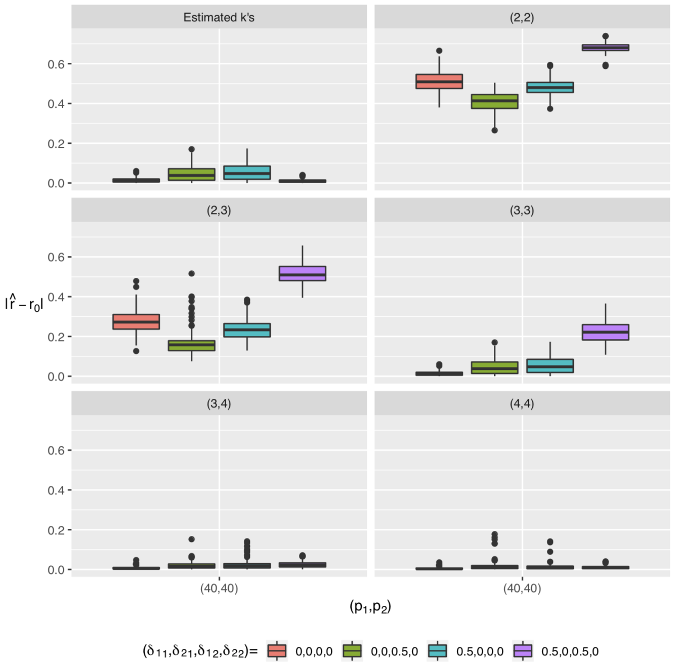
| , , , | ||||
|---|---|---|---|---|
| 0, 0 | 0, 0.5 | 0.5, 0 | 0.5, 0.5 | |
| 0.014 (0.011) | 0.047 (0.039) | 0.054 (0.039) | 0.011 (0.008) | |
| (4,4) | 0.005 (0.006) | 0.017 (0.024) | 0.013 (0.017) | 0.011 (0.008) |
| (4,3) | 0.007 (0.007) | 0.023 (0.026) | 0.020 (0.022) | 0.039 (0.022) |
| (3,4) | 0.008 (0.007) | 0.020 (0.017) | 0.024 (0.024) | 0.025 (0.016) |
| (3,3) | 0.014 (0.011) | 0.047 (0.039) | 0.054 (0.039) | 0.223 (0.052) |
| (4,2) | 0.314 (0.051) | 0.388 (0.048) | 0.440 (0.044) | 0.491 (0.053) |
| (2,4) | 0.274 (0.057) | 0.163 (0.056) | 0.236 (0.053) | 0.486 (0.049) |
| (3,2) | 0.312 (0.051) | 0.388 (0.049) | 0.433 (0.046) | 0.514 (0.051) |
| (2,3) | 0.273 (0.057) | 0.164 (0.060) | 0.237 (0.052) | 0.517 (0.049) |
| (2,2) | 0.509 (0.057) | 0.410 (0.047) | 0.481 (0.043) | 0.681 (0.024) |
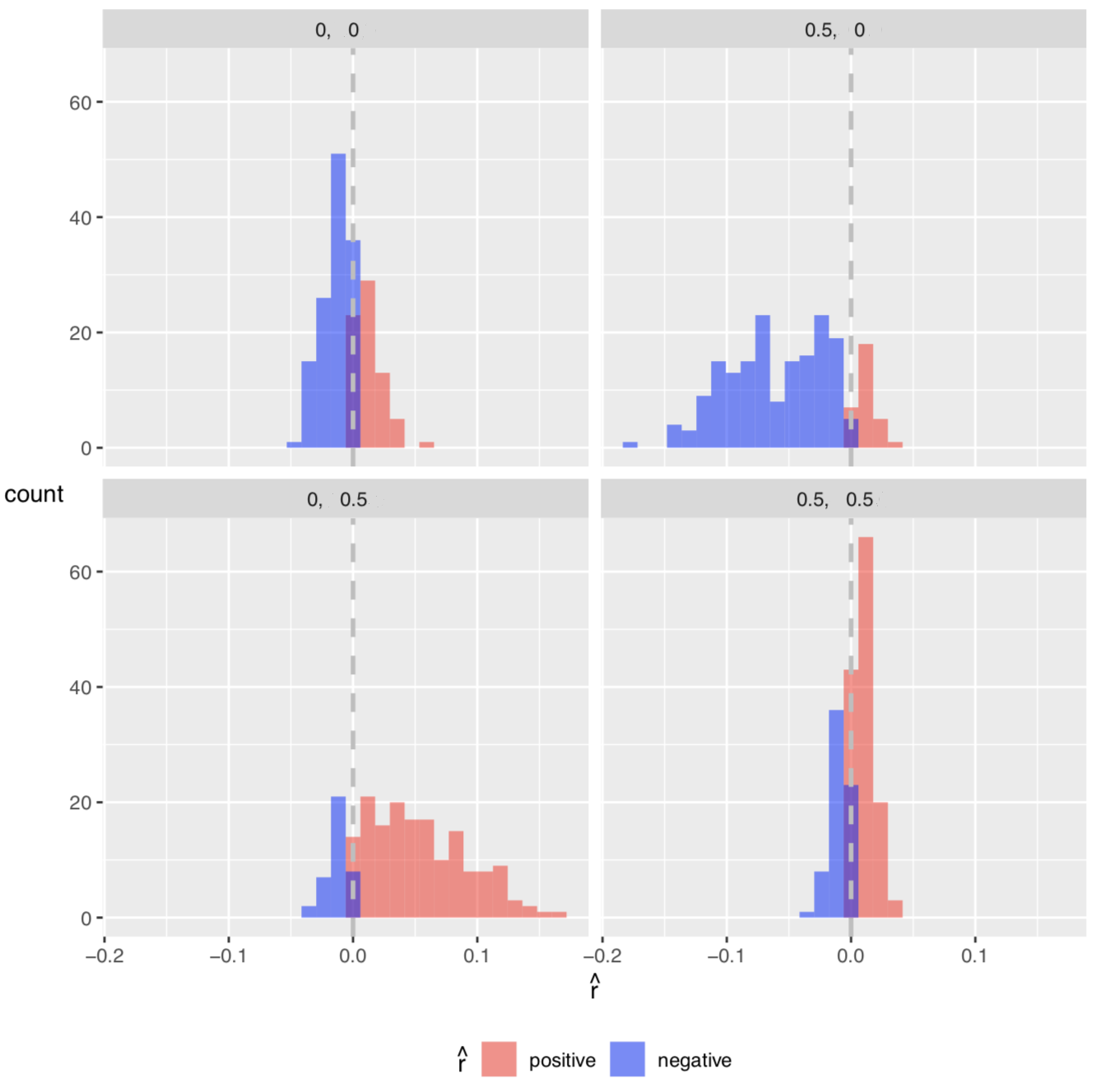
Figure 2 presents the histograms of with estimated by (34) when and . Different panels correspond to different combination of row strengths . From the figure, it is clear that tends to be biased towards negative when regime 1 () has a weak factor (top right figure) and tends to be biased towards positive when regime 2 () has a weak factor (bottom left), which confirms the conclusions in Theorem 2 and Theorem 4. The last figure at the bottom right shows tight concentration around true threshold value zero.
To investigate the bias in present of a single weak regime, we plot in Figure 3 for typical data sets under the four different settings in Table 1. We can observe that approaches the theoretical minimum value 0 of around when row factors are strong in at least one regime (Setting #1, 2, 3). When row factors are weak in both regimes (Setting #4), the range of is small, comparing with those in the other settings. Also, the minimum value of in Setting #4 is larger than 0, but it still occurs around . In Setting #2 and #3 where row factors have different levels of strength, is much large in the stronger regime. This also explains the existence of bias we observe in Figure 2.
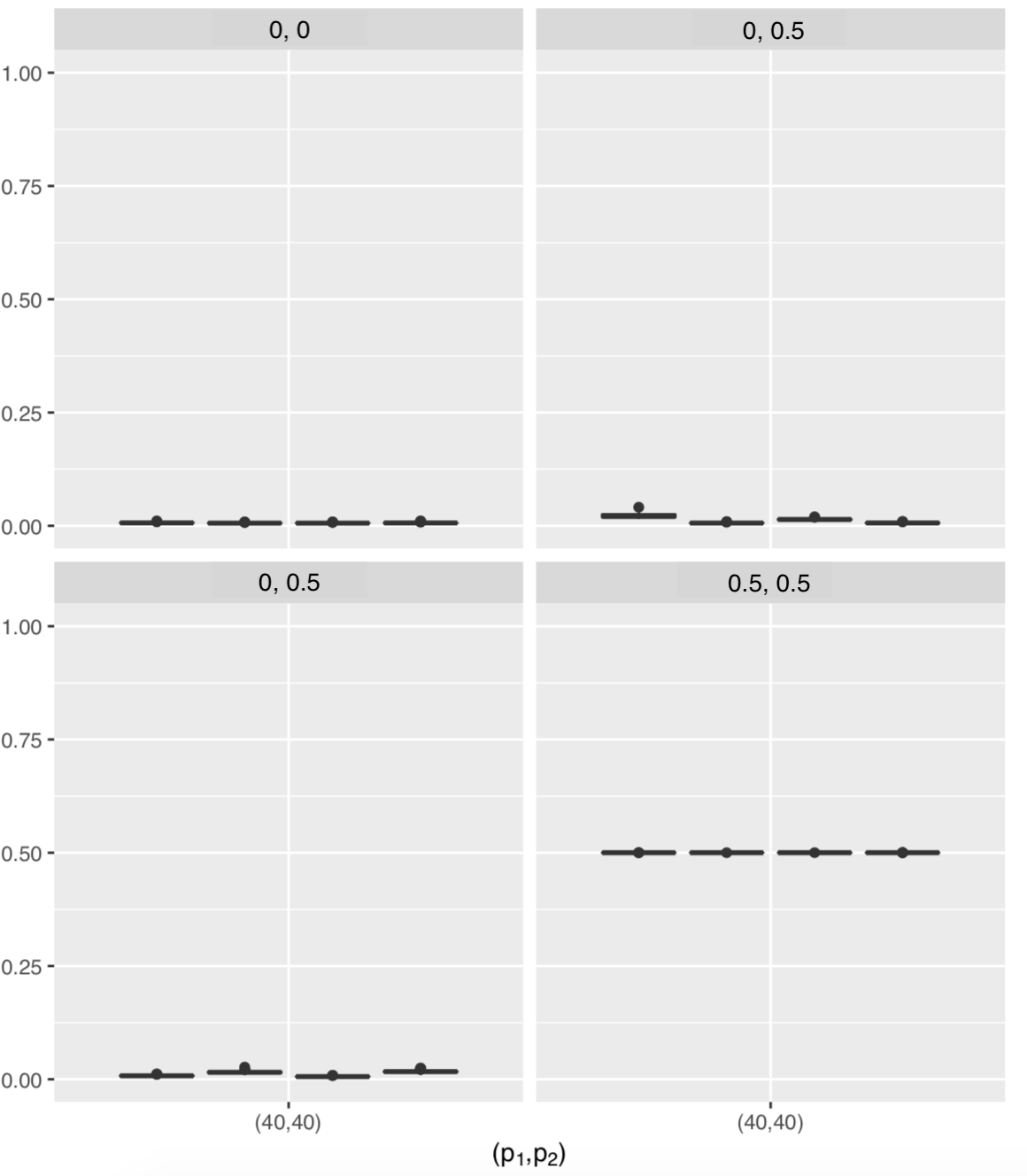
Thirdly, we investigate the accuracy in estimating the loading spaces when true , and are unknown. The pair is estimated by (34) and is estimated by (36). Then a representative matrix of the row or column loading space is estimated according to (37) for each regime. Figure 4 shows box plots of space distance for row and column loading matrices , , , and under different factor strength combinations. As shown in the top-left figure , when all factors are strong in both regimes, all loading spaces are estimated with high accuracy. As shown in the bottom-right figure , when both regimes have weak row factors, the estimated row loading spaces are away from the truth. The estimation of column loading spaces is also affected by the weak row factors. As shown in the top-right figure and bottom-left figure , when only one regime has a weak row factor, all loading spaces in the regime with the weak factor are estimated with lower accuracy than those in the regime with all strong factors. However, the discrepancies from the true loading spaces are smaller than those when both regimes contain strong factor.
4.2 Threshold Strength Helping Effect
The general phenomenon of the threshold strength helping effect in the threshold matrix factor model can be summarized as the fact that the row (column) loading with strong threshold strength can help with the column (row) loading with weak threshold strength. Thus at least one of row or column factors experiencing strong thresholding can guarantee an accurate estimation. This is aligned with the theoretical results presented in Theorem 2 and 3 and is again verified empirical through the synthetic data set.
In this example, we investigate the threshold strength effect as specified Condition 9 in Appendix A. Specifically, we consider different combinations of threshold strength summarized in Table 4. To ensure that the factors strengths and thresholding strengths are as we specify in Table 4, by the fact that is bounded by for any two orthonormal matrices and shown in Theorem 3 of Liu and Chen, 2016, we do the following: first generate two matrices and with all entries independently generated from the uniform distribution on , and let and ; then sample entries in and entries in , and replace them with new values independently generated from the uniform distribution on , where the new matrices are called and ; let and .
| Setting # | Row factor strength | Column factor strength | Row threshold strength | Column threshold effect | Interpretation | ||
| Regime 1 | Regime 2 | Regime 1 | Regime 2 | ||||
| 1 | 0 | 0 | 0 | 0 | 1 | 1 | Both row and column regimes are orthogonal. |
| 2 | 0 | 0 | 0 | 0 | 0.5 | 1 | Row regimes are orthogonal. Column regimes are close. |
| 3 | 0 | 0 | 0 | 0 | 0.5 | 0.5 | Both row and column regimes are close. |
| 4 | 0.5 | 0.5 | 0 | 0 | 1 | 1 | Both row and column regimes are orthogonal. |
| 5 | 0.5 | 0.5 | 0 | 0 | 0.5 | 1 | Row regimes are orthogonal. Column regimes are close. |
| 6 | 0.5 | 0.5 | 0 | 0 | 0.5 | 0.5 | Both row and column regimes are close. |
First, we examine the accuracy in estimating the number of factors and when true threshold value is unknown under different threshold strength. Table 5 shows the frequency of estimated pair obtained by (34). Here true threshold value is unknown, we use the sample points where is under 25-th percentile for regime 1 and those where is above 75-th percentile for regime 2 to estimate . As shown in the table, threshold strength does not affect the accuracy of the estimators . This is reasonable since the range of for separating regime 1 and regime 2 is correct. Thus is only affected by factor strength and efficient sample size – a quarter of the whole sample size for each , .
| (4,4) | (4,3) | (3,3) | |||||
|---|---|---|---|---|---|---|---|
| 40 | 40 | 2400 | 0,0,0,0 | 1,1 | 0 | 0 | 1.00 |
| 0.5,1 | 0 | 0 | 1.00 | ||||
| 0.5,0.5 | 0 | 0 | 1.00 | ||||
| 0.5,0.5,0,0 | 1,1 | 1.00 | 0 | 0 | |||
| 0.5,1 | 1.00 | 0 | 0 | ||||
| 0.5,0.5 | 0.99 | 0.01 | 0 |
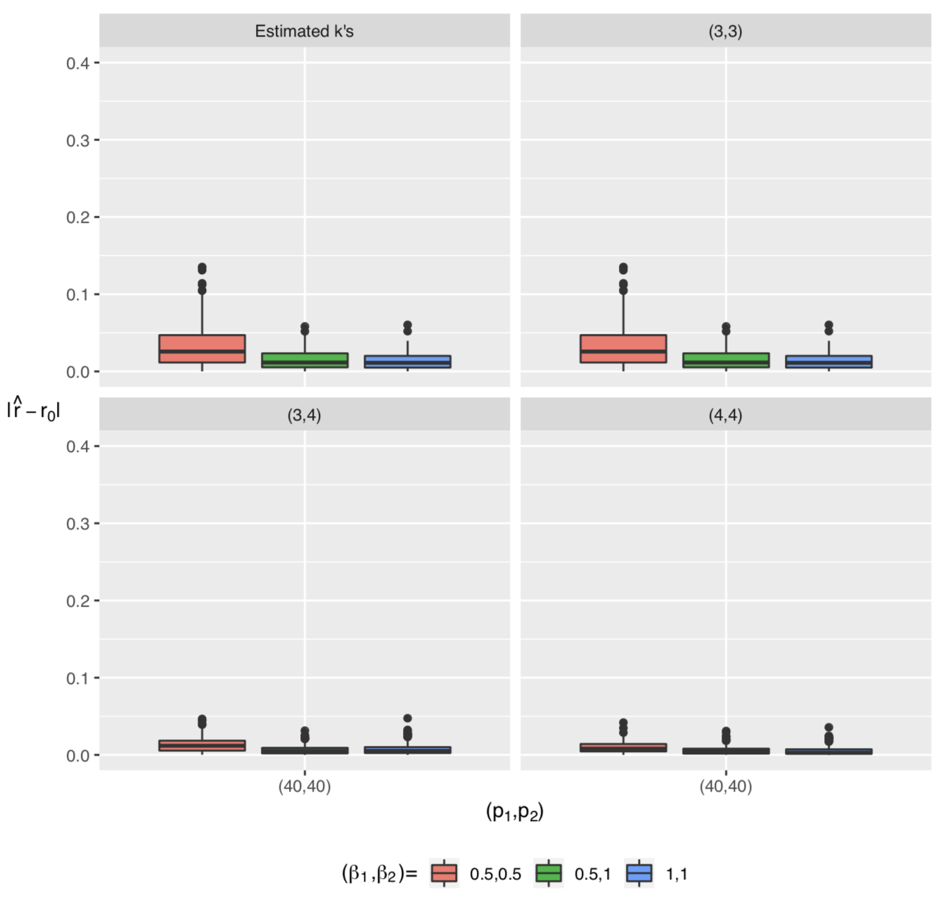
Secondly, we examine how different threshold strengths affect the recovery of the threshold value without knowing true latent dimensions. Figures 5 and 6 present the box plots of the absolute error under different threshold strength with and , respectively. The absolute error has smaller mean and variance under strong factors (Figure 5) than those under weak row factor (Figure 6). The performances for the cases where and are approximately the same, which is in line with conclusions in Theorem 2 and Theorem 4. Both are better than the case where . We called this phenomena the helping effect from the strong column thresholding to the weak row thresholding.
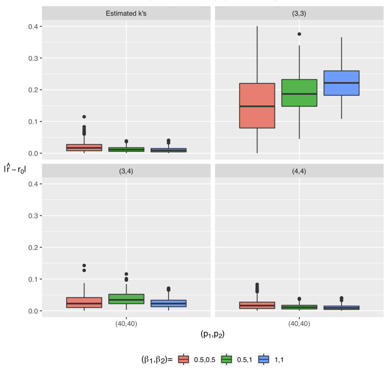
| , | ||||||
| 0,0,0,0 | 0.5,0.5,0,0 | |||||
| 1,1 | 0.5,1 | 0.5,0.5 | 1,1 | 0.5,1 | 0.5,0.5 | |
| 0.014(0.011) | 0.015(0.013) | 0.034(0.029) | 0.011(0.008) | 0.013(0.009) | 0.020(0.018) | |
| (4,4) | 0.005(0.006) | 0.006(0.006) | 0.01(0.007) | 0.011(0.008) | 0.013(0.009) | 0.020(0.016) |
| (4,3) | 0.007(0.007) | 0.013(0.010) | 0.015(0.011) | 0.039(0.022) | 0.095(0.053) | 0.121(0.078) |
| (3,4) | 0.008(0.007) | 0.007(0.006) | 0.014(0.010) | 0.025(0.016) | 0.037(0.021) | 0.028(0.024) |
| (3,3) | 0.014(0.011) | 0.015(0.013) | 0.034(0.029) | 0.223(0.052) | 0.191(0.058) | 0.160(0.103) |
| (4,2) | 0.314(0.051) | 0.520(0.048) | 0.056(0.041) | 0.491(0.053) | 0.616(0.059) | 0.065(0.039) |
| (2,4) | 0.274(0.057) | 0.358(0.037) | 0.092(0.046) | 0.486(0.049) | 0.468(0.048) | 0.093(0.033) |
| (3,2) | 0.312(0.051) | 0.517(0.048) | 0.061(0.040) | 0.514(0.051) | 0.623(0.057) | 0.064(0.039) |
| (2,3) | 0.273(0.057) | 0.357(0.038) | 0.098(0.049) | 0.517(0.049) | 0.502(0.047) | 0.105(0.039) |
| (2,2) | 0.509(0.057) | 0.589(0.044) | 0.080(0.040) | 0.681(0.024) | 0.630(0.043) | 0.079(0.037) |
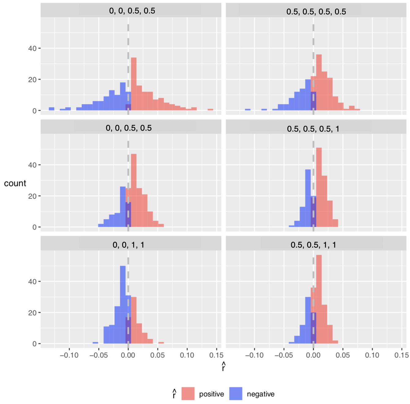
Figure 7 presents the histograms of with estimated by (34) under different combinations of factor strength and threshold strength . The title of each panel shows the value of . The three sub-figures in the left column all corresponds to the strong row and column factors case. The three sub-figures in the right column all corresponds to the weak row but strong column factors case. From the figure, it is clear that is not biased. This is because the factor strengths are the same in both regime. However, when the thresholding effects are weak for both row and column, i.e. , the variances of are larger. When the thresholding effects are strong for at least one of row or column loadings, i.e. or , concentrates around true threshold value zero. This again shows the the helping effect from the strong column thresholding to the weak row thresholding.
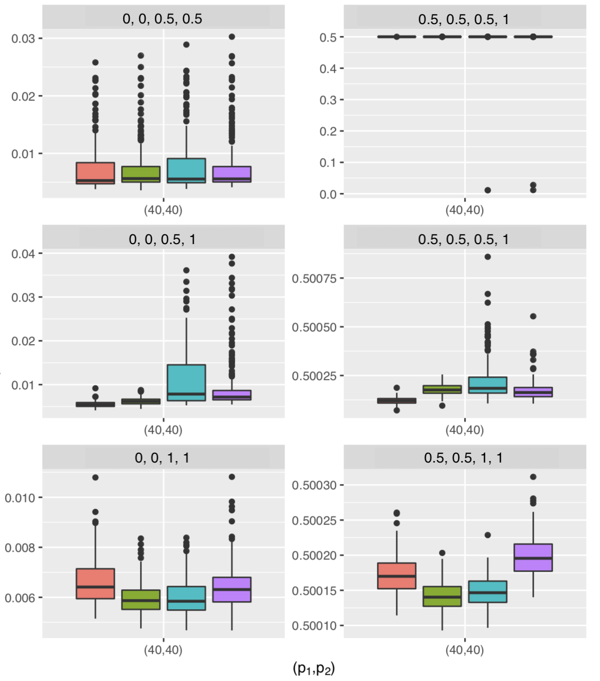
Thirdly, we investigate the accuracy in estimating the loading spaces when true , and are unknown. The pair is estimated by (34) and is estimated by (36). Then a representative matrix of the row or column loading space is estimated according to (37) for each regime. Figure 8 shows box plots of space distance for row and column loading matrices , , , and under different combinations of factor strength and thresholding strength . Panel title shows the value of . Note that to better present the variation of estimation errors in each setting, the sub-figures have different scales. As shown in the sub-figures in the left column with strong row/column factors in both regime, i.e. , all loading spaces are estimated with high accuracy. As shown in the the sub-figures in the right column with weak row but strong column factors in both regime, i.e. , the estimated row loading spaces are far from the truth. The thresholding strength affects the variance of the estimation. Estimation variances under strong thresholding are smaller than those under weak thresholding . The helping effect from the strong column thresholding to the weak row thresholding can be observed again by the case of with the cases of strong and weak threshold.
.
5 Application to Real Data
5.1 Example 1: Multinational Macroeconomic Indices
We apply the threshold matrix factor model to the multinational macroeconomic indices dataset in Chen et al., 2017. The dataset is collected from OECD. It contains 10 quarterly macroeconomic indices of 14 countries from 1990.Q2 to 2016.Q4 for 107 quarters. Thus, we have and matrix-valued time series. The countries include United States, Canada, New Zealand, Australia, Norway, Ireland, Denmark, United Kingdom, Finland, Sweden, France, Netherlands, Austria and Germany. The indexes cover four major groups, namely production (P:TIEC, P:TM, GDP), consumer price (CPI:Food, CPI:Ener, CPI:Tot), money market (IR:Long, IR:3-Mon), and international trade (IT:Ex, IT:Im). Each original univariate time series is transformed by taking the first or second difference or logarithm to satisfy the mixing condition (Condition 1 in Appendix A). See Table 9 in Appendix C for detailed descriptions of the dataset and the transformation. Figure 9 shows the transformed time series of macroeconomic indicators of multiple countries.
It is well known that there exists the pattern of expansion and contraction in macroeconomy. Here we analyzed the data using a 2-regime threshold factor model, intending to capture the expansion and contraction economic behaviros. Macroeconomic research has identified different groups of business cycle indicators. For example, leading indicators include average weekly work hours in manufacturing, factory orders for goods, housing permits, stock prices, the index of consumer expectations, average weekly claims for unemployment insurance and the interest rate spread; Coincident indicators include the unemployment rate, personal income levels and industrial production; Lagging indicators include the average length of unemployment, labor cost per unit of manufacturing output, the average prime rate, the consumer price index and commercial lending activity. We consider the each one in the groups of leading, coincident and lagging business cycle indicator for the the threshold value (with both leads and lags .) Namely, we use the OECD Composite Leading Indicator (CLI) from the leading indicator group, S&P500 return from the coincident indicator group, and the Consumer Price Index (CPI) from the lagging indicator group. Note that CPI and CLI are available for each country while our model use only one scalar threshold process . Since the countries in this data set are all developed countries from North American and European, the changes of business cycle are almost synchronous. We use the means of CLI and CPI across different countries.
Table 7 shows the value of for each candidate CLI, S&P500 squared return and CPI in different leads. Here, denotes transformation of first difference after logarithm. The threshold processes using CLI, S&P500 squared return, and CPI produce minimal ’s at lag 3, 1, and 3, respectively. In the following we use S&P500 squared return at time as the threshold variable for time , since it minimizes over all candidates.
| Threshold Process | ||||
|---|---|---|---|---|
| 8768.02 | 8715.37 | 8833.73 | 8824.84 | |
| 8710.79 | 8719.06 | 8734.01 | 8645.73 | |
| 8795.69 | 8743.94 | 8800.34 | 8848.71 |
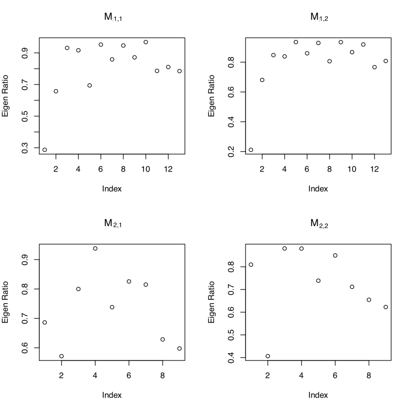
We use 25-th and 75-th percentiles of the threshold variable as and to estimate the number of factors. The four panels in Figure (10) display the ratio of eigenvalues of , , and , respectively. Ratio of the eigenvalues for row factors achieves its minimal at 1, while the ratio of eigenvalues for column factors achieves its minimal at 2. It yields that and .
To determine the threshold point , we estimate based on (35) and find the minimizer of the function. Figure 11(a) and Figure 11(b) show the plots of with estimated and overestimated . Both show U-shape curves with a relatively flat bottom. By minimizing , we have for both and . In this application, and . The two regimes are well separated.
Figure 12 shows sample time series in the multinational macroeconomic indices data set in two regimes. The proposed model gives very reasonable result. It shows clearly that Regime 1 corresponds to the high volatility periods and Regime 2 corresponds to low volatility periods.
5.2 Example 2: Fama-French 10 by 10 Series
In this section, we investigate threshold matrix-variate factor models for the monthly market-adjusted return series of Fama-French portfolios from January 1964 to December 2015 for 624 months and overall observations. The portfolios are the intersections of 10 portfolios formed by size (market equity, ME) and 10 portfolios formed by the ratio of book equity to market equity (BE/ME). Thus, we have and matrix-variate time series. The series are constructed by subtracting the monthly excess market returns from each of the original portfolio returns obtained from French, 2017, so they are free of the market impact.
Table 8 shows the value of for each threshold variable candidate including S&P500 return,S&P500 squared return, and their lag variables. The minimal of is achieved at S&P 500 return at lag 5. In the following we use it as the threshold variable.
| Threshold Process | ||||||
|---|---|---|---|---|---|---|
| 10629.75 | 10607.12 | 10933.95 | 11234.59 | 11262.81 | 10673.53 | |
| 11727.39 | 11264.92 | 11834.70 | 11678.43 | 11263.96 | 10845.61 |
We use 25-th and 75-th percentiles of the threshold variable as and to estimate the number of factors. The four panels in Figure 13 display the ratio of eigenvalues of , , and , respectively. Eigen-ratio for both row and column factors achieve minimal at 1. It yields that and .
To determine the threshold point , we estimate based on (35) and find the to minimize the function. Figure 14(a) and Figure 14(b) show the plots of with estimated and overestimated . Both show U-shape curves with a relatively flat bottom. By minimizing , we have for and for , which are very close. In this application, and . Since the separation between these two regimes is moderate, we use overestimated dimension in the following steps.
Figure 15 shows sample time series in the monthly Fama-French data set in two regimes. It shows clearly that Regime 1 corresponds to the low return periods and Regime 2 corresponds to high return periods.
6 Summary and Future Work
In this article, we propose a threshold factor models for high-dimensional matrix-valued time series data. The loading spaces are allowed to change across regimes controlled by a threshold variable. The procedures to estimate threshold value, loading spaces in different regimes, and the number of factors are developed. The asymptotic properties of the estimators are investigated. We found that the strengths of factors in different regimes and the strength of thresholding play an important role in estimation results. When factors and thresholding are all strong, our estimation is immune to the curse of dimensionality. When the factors and thresholding are not all strong, the estimation of loading spaces and threshold value experience the ’helping’ effect against the curse of dimensionality. The loading space estimation in the weaker regime gain efficiency and the impact of the curse of dimensionality is reduced due to the existence of a stronger regime. Comparing vector-valued factor models, the estimation of threshold value in matrix-valued models also benefits by introducing a direction with stronger thresholding. Determining the number of factor is a challenging issue for factor analysis. In this paper, we show that the proposed estimators are consistent even if the number of factors is overestimated.
Many potential research projects related to this topic have been left for future work. We only study two-regime models in this paper. It would be interesting to consider factor models with multiple regimes, and develop procedures for regime detection. Furthermore, we could also extend our approach for matrix time series analysis to tensor time series analysis, which is an interesting and new research direction.
References
- Bai et al., (2017) Bai, J., Han, X., and Shi, Y. (2017). Estimation and inference of change points in high-dimensional factor models. Working paper.
- Bai and Ng, (2002) Bai, J. and Ng, S. (2002). Determining the number of factors in approximate factor models. Econometrica, 70:191–221.
- Barigozzi et al., (2018) Barigozzi, M., Cho, H., and Fryzlewicz, P. (2018). Simultaneous multiple change-point and factor analysis for high-dimensional time series. Journal of Econometrics, 206:187–225.
- Breitung and Eickmeier, (2011) Breitung, J. and Eickmeier, S. (2011). Testing for structural breaks in dynamic factor models. Journal of Econometrics, 163:71–84.
- Chamberlain and Rothschild, (1983) Chamberlain, G. and Rothschild, M. (1983). Arbitrage, factor structure and mean-variance analysis in large asset markets. Econometrica, 70:191–221.
- Chan, (1993) Chan, K. (1993). Consistency and limiting distribution of the least squares estimator of a threshold autoregressive model. The Annals of Statistics, 21:520–533.
- Chang et al., (2015) Chang, J., Guo, B., and Yao, Q. (2015). High dimensional stochastic regression with latent factors, endogeneity and nonlinearity. Journal of Econometrics, 189:297–312.
- Chen et al., (2017) Chen, E. Y., Tsay, R. S., and Chen, R. (2017). Constrained factor models for high-dimensional matrix-variate time series. ArXiv e-prints.
- Chen et al., (2014) Chen, L., Dolado, J., and Gonzalo, J. (2014). Detecting big structural breaks in large factor models. Journal of Econometrics, 180:30–48.
- Cunha et al., (2010) Cunha, F., Heckman, J., and Schennach, S. (2010). Estimating the technology of cognitive and noncognitive skill information. Econometrica, 78:883–931.
- Fan et al., (2016) Fan, J., Liao, Y., and Wang, W. (2016). Projected principal component analysis in factor models. The Annuals of Statistics, 44:219–254.
- Fan et al., (2017) Fan, J., Xue, L., and Yao, J. (2017). Sufficient forecasting using factor models. Journal of Econometrics, 201:292–306.
- Fan and Yao, (2003) Fan, J. and Yao, Q. (2003). Nonlinear Time Series: Nonparametric and Parametric Methods. Springer-Verlag, New York.
- Forni et al., (2000) Forni, M., Hallin, M., Lippi, M., and Reichlin, L. (2000). The generalized dynamic factor model: identification and estimation. Review of Economics and Statistics, 82:540–554.
- Forni and Reichlin, (1998) Forni, M. and Reichlin, L. (1998). Let’s get real: a factor-analytical approach to disaggregated business cycle dynamics. Review of Economic Studies, 65:453–473.
- French, (2017) French, K. R. (2017). 100 Portfolios Formed on Size and Book-to-Markete. http://mba.tuck.dartmouth.edu/pages/faculty/ken.french/Data_Library/det_100_port_sz.html. [Online; Accessed 01-Jan-2017].
- Geweke, (1977) Geweke, J. (1977). The dynamic factor analysis of economic time series. Latent variable in socio-economic models, ed. by D.J. Aigner and A.S. Goldberg, Amsterdam: North Holland.
- Hallin and Liska, (2007) Hallin, M. and Liska, R. (2007). Determining the number of factors in the general dynamic factor model. Journal of the American Statistical Association, 102:603–617.
- Han and Inoue, (2015) Han, X. and Inoue, A. (2015). Tests for parameter instability in dynamic factor models. Econometric Theory, 31:1117–1152.
- Lam and Yao, (2012) Lam, C. and Yao, Q. (2012). Factor modeling for high-dimensional time series: inference for the number of factors. Annals of Statistics, 40(2):694–726.
- Lam et al., (2011) Lam, C., Yao, Q., and Bathia, N. (2011). Estimation of latent factors for high-dimensional time series. Biometrika, 98(4):901–918.
- Lee and Shao, (2018) Lee, C. and Shao, X. (2018). Volatility martingale difference divergence matrix and its application to dimension reduction for multivariate volatility. Journal of Business & Economic Statistics, pages 1–13.
- Liu and Chen, (2016) Liu, X. and Chen, R. (2016). Regime-switching factor models for high-dimensional time series. Statistica Sinica, 26:1427–1451.
- Liu and Chen, (2019) Liu, X. and Chen, R. (2019). Threshold factor models for high-dimensional time series. Manuscript, Available at arXiv: 1809.03643.
- Ma and Su, (2018) Ma, S. and Su, L. (2018). Estimation of large dimensional factor models with an unknown number of breaks. Journal of Econometrics, 207:1–29.
- Massacci, (2017) Massacci, D. (2017). Least squares estimation of large dimensional threshold factor models. Journal of Econometrics, 197:101–129.
- Merikoski and Kumar, (2004) Merikoski, J. K. and Kumar, R. (2004). Inequalities for spreads of matrix sums and products. Applied Mathematics E-Notes, 4:150–159.
- Pan and Yao, (2008) Pan, J. and Yao, Q. (2008). Modelling multiple time series via common factors. Biometrika, 95:365–379.
- Peña and Box, (1987) Peña, D. and Box, G. E. P. (1987). Identifying a simplifying structure in time series. Journal of the American statistical Association, 82:836–843.
- Peña and Poncela, (2006) Peña, D. and Poncela, P. (2006). Nonstationary dynamic factor analysis. Journal of Statistical Planning and Inference, 136:1237–1257.
- Shumway and Stoffer, (2017) Shumway, R. and Stoffer, D. (2017). Time series analysis and its applications with R examples. Springer.
- (32) Stock, J. H. and Watson, M. W. (2002a). Forecasting using principal components from a large number of predictors. Journal of the American Statistical Association, 97:1167–1179.
- (33) Stock, J. H. and Watson, M. W. (2002b). Macroeconomic forecasting using diffusion indices. Journal of Business & Economic Statistics, 20:147–162.
- Su and Wang, (2017) Su, L. and Wang, X. (2017). On time-varying factor models: estimation and testing. Journal of Econometrics, 198:84–101.
- Tong, (1990) Tong, H. (1990). Nonlinear time series: a dynamic system approach. Clarendon Press, Oxford.
- Tong and Lim, (1980) Tong, H. and Lim, K. (1980). Threshold autoregression, limit cycles and cyclical data. Journal of the Royal Statistical Society: Series B (Statistical Methodology), 42(3):245–292.
- Tsay, (1989) Tsay, R. (1989). Testing and modeling threshold autoregressive process. Journal of the American Statistical Association, 84:231–240.
- Tsay, (1998) Tsay, R. (1998). Testing and modeling multivariate threshold models. Journal of the American Statistical Association, 93:1188–1202.
- Wang et al., (2019) Wang, D., Liu, X., and Chen, R. (2019). Factor models for matrix-valued high-dimensional time series. Journal of Econometrics, 208:231–248.
- Yalcin and Amemiya, (2001) Yalcin, I. and Amemiya, Y. (2001). Nonlinear factor analysis as a statistical method. Statistical Science, 16:275–294.
Appendix A Regularity Conditions
Define
Condition A1. The process is -mixing. Specifically, for some , the mixing coefficients satisfy the condition , where
and is the -field generated by .
Condition A2. Let be the -th entry of . For any , , and , , where is a positive constant and is given in Condition A1. There exists an such that , and is uniformly bounded, where , as and go to infinity and and are fixed. For and , , .
Condition A3. The absolute value of each element in remains bounded by as and increase to infinity for . and for .
We do not impose stationarity assumptions for the factor process and the noise process , but should satisfy the mixing condition as specified in Condition A1. Condition A2 ensures that the autocovariance matrices contain useful information from different fundamental factors and the model is not redundant. Condition A3 allows the noise process to accommodate strong cross-sectional dependence by only imposing entry-wise constraints on its covariance matrix. Under Condition A3, is an exogenous and independent process.
Condition A4. For , there exist constants and such that and , as and go to infinity and and are fixed.
Condition B1. Assume is a continuous random variable and the process is stationary. The marginal probability of satisfies that and . and for and .
Conditions B1 guarantees that there is enough information in partial data with for loading space estimation.
Condition B2. There exists a positive integer such that and is uniformly bounded above 0, for .
Condition B3. has distinct positive eigenvalues for .
can be viewed as the signal part of the observation , and as the noise. The signal strength, or the strength of the factors, can be measured by the -norm of the loading matrices which is assumed to grow with the dimensions. The constants in Condition A4 control the strength levels of factors. Condition B2 implies that autocovariance matrices in both regimes account for , and guarantees the ’helping’ effect since the one corresponding to the strong regime carries more information about and improves the estimation efficiency. Under Condition B3, we can unique define , where and is the unit eigenvector of corresponding to the -th largest eigenvalue.
Condition C1. Assume . is a continuous random variable, and the process is stationary. The marginal probability of satisfies that and . The densities of , is continuous, and there exist two positive constants and such that uniformly in . The conditional probability of satisfies that and for any or and .
Condition C2. There exists a positive integer such that and is uniformly bounded above 0, for .
Condition C3. has distinct positive eigenvalues for .
Condition C4. There exists a positive integer such that and is uniformly bounded above 0, for .
Condition C5. has distinct positive eigenvalues for .
Condition C6. For any , there exists an integer such that and . For any , there exists an integer such that and . The minimum nonzero singular values of these four matrices mentioned are all uniformly bounded above , where .
Condition C1-3 indicate that the estimators for loading spaces are consistent when only data with are used. Condition C4 is a natural generalization of Condition B3 and avoid a redundant model. Condition C5 uniquely defines for . Condition C6 guarantees that the autocovariance matrices of with mixed data from two regimes carries all the information from the latent factor process.
Condition C7. Strength of thresholding. and . There exists two positive constants such that and .
and reflect the growth rate of the distances of loading spaces as and go to infinity. It also measures how much the thresholding effect experiences. If , only a finite number of elements in and are different across regimes when and go to infinity; if , the number of elements which undergo a change is , for .
Condition C8. When there exists two positive constants and such that and , where is a matrix, for and any matrix such that .
If the numbers of factors are overestimated, Condition C8 implies that the two augmented loading spaces and are still differentiable for .
Appendix B Lemmas and Proofs
In the appendix, only the theoretical results for are demonstrated, since those for are similar. Moreover, we mainly focus on the proofs when and because those for or can be obtained in a similar fashion. We use ’s and ’s to denote generic uniformly positive constants which only depend on the parameters.
Let be the common component of , i.e., . It can also be written as . Define
Lemma 1.
Let denote the -th entry in . Under Conditions A1-A2 and C1, for any , and , if holds that
and
where , and can be any real numbers in , , or . if at least one of them is or , and if and are both real numbers, where is given in Condition C1.
Proof: Condition C1 indicates that for . By Condition A2 and Jensen’s inequality we can show that , , and for , and . Under Conditions A1 and A2, by Proposition 2.5 in Fan and Yao, 2003, we have
and
Lemma 2.
For , , it holds that
and
where can be real numbers, , or .
Proof: By the definition and properties of Kronecker product, we have
The other inequality can be proven similarly.
Lemma 3.
Under Conditions A1-A2, A4 and C1, for , it holds that
and
where satisfies for , and can be real numbers in , or .
Proof: Condition A4 implies that there exists a positive constant such that for . By Lemma 1 and Lemma 2, it follows
We can also obtain the bound of with Lemma 1 and Lemma 2,
Lemma 4.
Under Conditions A1-A4 and C1, for and any , it holds that
where , , , and satisfies and for .
Proof: By Condition A4, we can find a positive constant such that and for . By Lemmas 1 and 3, when and ,
For the interaction of the common component and noise,
| (38) | |||||
and similarly we have
For the noise term,
It follows
where , , and .
For other cases, we can prove it in a similar way.
Lemma 5.
Under Conditions A1-A4 and C1, for , we have
when and ,
Proof: By the definition of and Lemma 3, if , we have
Other equations can be obtained in a similar fashion.
Lemma 6.
Under Conditions A4 and C7, it holds that
and
where and are positive constants such that , for , and is a positive constant such that for .
Proof. Note that
On the other hand,
Hence, . Then Condition C7 indicates that we can find two positive constants and such that . Therefore, and . With Condition A4, we have
Lemma 7.
Under Conditions A1-A4, C5, and C7 for , we have
Proof: If , by the definition, we have
If , by the definition, we have for . Hence, there exists a orthogonal matrix such that . By Lemmas 3 and 6 and Cauchy-Schwarz inequality,
Lemma 8.
Under Conditions A1-A4 and C6-C7, for any ,
and for any ,
where is the -th largest eigenvalue of .
Proof: By definition and properties of Kronecker product, we have
Under Conditions A1-A3, following the proof of Lemma 5 in Wang et al., 2019, we can obtain
Since is a symmetric positive definite matrix, we can find a positive definite matrix such that and , for , where is defined in Lemma 6. With the property of Kronecker product, it can be seen that . By Theorem 9 in Merikoski and Kumar, 2004, Lemma 3, and Condition C6, we have .
Proof of Theorem 1. When and and and are fixed, under Conditions A4 and B1, similar to Lemmas 1, and 3-5, we can show that
and
Since since , by Cauchy-Schwarz inequality, it follows
Similar to Lemma 8, with Condition B2 we can prove that there exists a positive constant such that for . By Theorem 9 in Merikoski and Kumar, 2004, we have
| (46) | |||||
Since , we know that . Following the proof for Theorem 1 in Lam et al., 2011 and Theorem 3 in Liu and Chen, 2016, we have ).
Lemma 9.
Under Conditions A1-A4 and C1-C7, for , with true , when and are large enough, we have , and
where .
Proof: When , if , when and are large enough by Theorem 9 in Merikoski and Kumar, 2004 and Lemmas 3, 6, and 8, we have
If as , , and go to infinity, then we have
In sum, when and are large enough we have
where . We can also show that
It indicates that
It can be shown that when and by definition and Lemmas 7 and 8.
Lemma 10.
Under Conditions A1-A4 and C1-C3, if , with true , as , it holds that
where is a generic uniformly positive constant which only depends on the parameters.
Proof: Let , and are real numbers in , , or . Condition A2 and Jensen’s inequality indicate that , , and . Thus, by Cauchy-Schwartz inequality, Proposition 2.5 in Fan and Yao, 2003 and Lemma 1,
Together with Lemma 2, we have
| (48) | |||||
Define
(48) shows
For the interaction of the common component and noise, with (38) we can show in a similar way that
and
For the noise term,
Similar to the proof of Lemma 4, it can be shown that there exists a positive constant such that
for , where and do not depend on , , or .
If , we have
Together with (46), following the proof for Theorem 1 in Lam et al., 2011 and Theorem 3 in Liu and Chen, 2016, we can reach the conclusion.
Lemma 11.
Under Condition A1-A4 and C1-C7, with true , when ,
when ,
and
Proof: Since , by the definition, for . Hence, there exists a orthogonal matrix such that . Then we have
| (49) | |||||
When , by Cauchy-Schwarz inequality and Lemmas 4-7 and 10,
and
It follows from (49),
Similarly we can establish the rate of convergence for . Then when , we have
where .
Proof of Theorem 2. Let . Following the proof of Theorem 2 in Liu and Chen, 2019, we can reach the conclusion.
Proof of Theorem 3. When , if , by Cauchy-Schwarz inequality and Lemmas 4-5, we have
| (50) | |||||
Under Condition A4, it follows from Lemma 3,
and
Hence,
If , together with (50), we have
Theorem 2 states that if , . Therefore,
| (51) |
On the other hand, under Condition C4 following the proof of Lemma 8, we can obtain
If , by Theorems 6 and 9 in Merikoski and Kumar, 2004, we can show that
If as and go to infinity,
Hence, . Similar to the proof of Theorems 1 in Lam et al., 2011 and Theorem 3 in Liu and Chen, 2016, with (51), the conclusions can be reached.
Lemma 12.
For , let be a orthogonal matrix such that for . Under Conditions A1-A4 and C1-C8, for any , it holds that
Proof: Similar to proof of Lemma 7 in Liu and Chen, 2019.
Proof of Corollary 1. Similar to proof of and Corollary 1 in Liu and Chen, 2016.
Proof of Theorem 4. With Lemma 12, following the proof of Theorem 4 in Liu and Chen, 2019, we can reach the conclusion.
Proof of Theorem 5. Similar to proof of Theorem 3.
Appendix C Multinational Macroeconomic Indexes Dataset
Table 9 lists the short name of each series, its mnemonic (the series label used in the OECD database), the transformation applied to the series, and a brief data description. All series are from the OECD Database. In the transformation column, denote the first difference, denote the first difference of the logarithm. GP denotes the measure of growth rate last period.
| Short name | Mnemonic | Tran | description |
|---|---|---|---|
| CPI: Food | CPGDFD | Consumer Price Index: Food, seasonally adjusted | |
| CPI: Ener | CPGREN | Consumer Price Index: Energy, seasonally adjusted | |
| CPI: Tot | CPALTT01 | Consumer Price Index: Total, seasonally adjusted | |
| IR: Long | IRLT | Interest Rates: Long-term gov bond yields | |
| IR: 3-Mon | IR3TIB | Interest Rates: 3-month Interbank rates and yields | |
| P: TIEC | PRINTO01 | Production: Total industry excl construction | |
| P: TM | PRMNTO01 | Production: Total manufacturing | |
| GDP | LQRSGPOR | GDP: Original (Index 2010 = 1.00, seasonally adjusted) | |
| IT: Ex | XTEXVA01 | International Trade: Total Exports Value (goods) | |
| IT: Im | XTIMVA01 | International Trade: Total Imports Value (goods) |
| Country | ISO ALPHA-3 Code | Country | ISO ALPHA-3 Code |
|---|---|---|---|
| United States of America | USA | United Kingdom | GBR |
| Canada | CAN | Finland | FIN |
| New Zealand | NZL | Sweden | SWE |
| Australia | AUS | France | FRA |
| Norway | NOR | Netherlands | NLD |
| Ireland | IRL | Austria | AUT |
| Denmark | DNK | Germany | DEU |