Naphthalene crystal shape prediction from molecular dynamics simulations
Abstract
We used molecular dynamics simulations to predict the steady state crystal shape of naphthalene grown from ethanol solution. The simulations were performed at constant supersaturation by utilizing a recently proposed algorithm [Perego et al. J. Chem. Phys., 142, 2015, 144113]. To bring the crystal growth within the timescale of a molecular dynamics simulation we applied Well-Tempered Metadynamics with a spatially constrained collective variable, which focuses the sampling on the growing layer. We estimated that the resulting steady state crystal shape corresponds to a rhombic prism, which is in line with experiments. Further, we observed that at the investigated supersaturations, the face grows in a two step two dimensional nucleation mechanism while the considerably faster growing faces and grow new layers with a one step two dimensional nucleation mechanism.
1 Introduction
Controlling the crystal shape of organic molecules is crucial for process optimization in a wide range of industries, in particular in the pharmaceutical industry. Active pharmaceutical ingredients (APIs) are commonly produced as crystal powders purified by crystallization from solution in stirred suspension crystallizers. The resulting crystal shape affects among other properties the filterability, tabletability, and bio-availability of the drug product. Hence, control of the crystal shape is crucial in the manufacturing of pharmaceutical compounds [1, 2]. Experimental methods aimed at determining the crystal shape are often expensive and cumbersome. For this reason optimizing the crystallization conditions to obtain the desired crystal shape can be a laborious trial-and-error endeavor. Obtaining insight into the growth process at the molecular level would be useful to make a rational choice for the crystallization conditions.
Molecular dynamics (MD) simulations have recently emerged as a useful tool to obtain atomistic insight into crystal growth [3, 4, 5, 6, 7, 8, 9, 10]. In particular, the work of Salvalaglio et al. [11] showed the usefulness of MD simulations for the paradigmatic case of urea. In that work, the growth rate was calculated and the growth mechanisms, rough growth or two dimensional (2D) nucleation, were identified from simulations in which the crystal surface of interest was exposed to a supersaturated solution. Afterwards, the crystal shape was predicted based on the relative growth rates of the different crystal faces [12].
The present work is dedicated to the study of naphthalene crystal growth in ethanol solution under different supersaturations[13, 14]. After urea, naphthalene is a step further towards the simulation of systems as complex as real life APIs.
The study of crystal growth of naphthalene using MD simulations presents at least two major challenges. First, the growth rates of the slowest growing crystal faces of naphthalene are so small, that growth of new layers is not observable within the timescale of a standard MD simulation ( 1 s). To overcome the simulation time limitation we employ Well-Tempered Metadynamics [15] (WTMetaD), which is a well established enhanced sampling method for the study of rare events.
Secondly, the strong finite size effects hamper direct comparison with experiments. For instance, typical experiments are performed at approximately constant supersaturation while standard MD simulations are unable to maintain such conditions [8, 11]. The finite size effects are addressed using the constant chemical potential molecular dynamics (CMD) method developed by Perego et al. [16], which maintains a constant supersaturation in the region adjacent to the crystal. With this simulation setup, relative growth rates of faces growing in the 2D nucleation regime can be obtained as a function of supersaturation.
2 Methods
2.1 Chemical potential control
In this section, we briefly summarize the CMD method. Further details can be found in Reference [16]. The main features of this method are schematically depicted in Figure 1: The system has periodic boundary conditions in all directions and is segmented along the -axis into one reservoir, two control regions, as well as transition regions which surround the crystal slab. The slab is oriented such that the face of interest is exposed to the solution along the -axis.
The method works as follows: Two forces, and , are introduced in order to control the flux of molecules between the reservoir and the left and right control regions, respectively. Each force acts along the -axis at a distance from the crystal surface position , namely at positions and , where . The functional forms of the forces are
| (1) | ||||
| (2) |
where is the time, and denote the instantaneous solute concentrations, while and are the predefined set-values of the concentration in the left and right control regions respectively. is a force constant, and corresponds to the bell-shaped function defined as
| (3) |
whose height and width are controlled by the parameter .
The idea behind the method is that depending on the concentration in the control regions at time , will accelerate the molecules towards or away from the control regions. In this way, the concentration in the control regions can be kept constant.
2.2 Metadynamics
The crystal growth rate depends on the growing crystallographic plane and the solution supersaturation. In the case of naphthalene, even at high supersaturations, the growth of certain faces takes place in timescales much longer than those that can be afforded using standard MD simulations. Here, we shall use WTMetaD, to bring the growth event within the timescale of the simulation. In this approach, a bias potential that evolves in time is constructed as a function of a small number of collective variables (CVs) , which are functions of the atomic coordinates. The objective of is to discourage frequently visited configurations and aid the system to surmount free energy barriers. is defined as a sum of Gaussian functions of height and width . converges asymptotically to [17]
| (4) |
where is the free energy surface (FES); is the so called bias factor, which takes a value greater than 1, and dictates how fast the height of the Gaussian functions decays with time. The time dependent energy offset is independent on . The FES can be calculated as a function of a different set of CVs using the reweighting procedure decribed in Reference [18]. The interested reader is referred to References [15] and [17] for further details on WTMetaD.
2.3 Surface layer crystallinity
An important ingredient of WTMetaD is the choice of CVs. The CVs are typically non-linear functions of the atomic coordinates and describe the progress (state) of the process under study. In the case of crystallization, a reasonable choice is to use as CV the number of crystalline molecules in the growing layer. This CV would enhance both the growth and the dissolution of a single layer on the surface of the seed crystal. Here, we shall use a simple yet effective modification of the CV described in Reference [8] to localize the CV to the growing surface layer.
The CV should be able to account for the fact that molecules have a different environment in solution and in the crystal [19]. Molecules in solution are characterized by a small coordination number and almost random relative orientation of the neighbors. On the other hand, molecules in the crystal have higher coordination numbers and are aligned with respect to their neighbors. With this in mind, we define the surface layer crystallinity of solute molecule as
| (5) |
where the function localizes the CV to the surface layer, describes the local density, and the local order.
The CV needs to be continuous and differentiable. Function is defined for each solute molecule to have a non-zero value if solute molecule is located within the surface layer. Defining the -axis as perpendicular to the crystal surface, takes the form
| (6) |
where is the position of molecule along the -axis, and determine the boundaries of the surface layer, while and define the steepness of individually on the crystal and on the liquid side of the surface layer. Figure 2a shows a snapshot of a simulation box of the face of naphthalene in which the surface layer is shaded in red. The as a function of for this configuration is shown below.
The local density is defined with the following rational switching function
| (7) |
where is the coordination number of molecule , a predefined threshold value, and a parameter that determines the steepness of the switching function. If surpasses , tends to 1, whereas otherwise it tends to 0; is defined as
| (8) |
where is the number of solute molecules in the system and is defined for solute molecule pairs and as
| (9) |
Function , which was introduced in Equation (6), provides non-zero values only for neighboring molecules within the surface layer. The distance between the molecule pair is given by and is the cutoff for the calculation of the coordination number.
Now we turn to describe the part of that characterizes the local order. The orientation in space of each molecule is characterized by a vector l. In the case of naphthalene, l is defined along the long axis of the molecule, see Figure 2b. The relative orientation between solute molecules and is characterized through an angle defined as In Figure 2c we show the probability density function of for neighbors inside the cutoff both for the liquid and the crystalline phase of naphthalene. The histogram shows four well defined peaks, each peak corresponding to one of the reference angles present in the crystal. We can now define the local order in Equation (5) as
| (10) |
where is the width of the angular distribution associated to . denotes the total number of reference angles occurring in the crystal. The purpose of in Equation (10) is to restrict the summation on only to the neighbors within . Also, dividing by normalizes in the interval . Values of close to 1 correspond to an environment where neighbors are aligned according to the reference angles , while values of close to 0 characterize environments with random orientations relative to their neighbors.
The combined effect of , , and leads to a crystallinity measure that takes into account both density and order around the molecule within the surface layer. Taking the sum over all solute molecules of the system leads to the surface layer crystallinity
| (11) |
which quantifies the crystallinity of the growing layer and avoids distortions of the bulk liquid as well as the bulk crystal in biased simulations by the use of the function . In Figure 2d we show probability density functions (PDFs) of for a fully liquefied layer and for a fully grown crystal layer. It is clear from the figure that distinguishes well these two states.

2.4 Biased collective variable
Although could have been used to construct the WTMetaD bias potential, we found it beneficial to use a slightly different CV. This is due to the fact that the two minima in the FES corresponding to the fully dissolved layer (A) and fully grown layer (B) have rather different widths (see the illustrative scheme in Figure 3a). In particular basin A is rather narrow and close to the boundary of the CV. The first feature requires the use of very narrow Gaussians. These narrow Gaussians are totally unnecessary in the filling of basin B and thus convergence is slowed down. On the other hand, the closeness of basin A to the boundary creates artificial effects [20, 21].
In order to solve these problems, we could have used the variable Gaussian width approach of Branduardi et al. [22]. Here instead we prefer to use a much simpler fixup. We use as CV not directly but the power law modification
| (12) |
where the exponent 1 is chosen to make the two minima approximately equally broad. A qualitative example of the effect of this change of CV is shown in Figure 3b. Not only are the two minima similarly broad but the minimum at A has been pushed fundamentally from the = 0 border. Adapting the CV in this way leads to an improved sampling of the low crystallinity states, while not affecting the sampling of high crystallinity states in an undesired manner.
The parameters used for , , and WTMetaD are tabulated in the supporting information (SI).
2.5 Force fields
The general AMBER force field (GAFF) [23, 24] was used for naphthalene and ethanol. Both types of molecules have a fully atomistic description. For naphthalene, the relaxed structure and the restrained electrostatic potential (RESP) charges [25] were calculated with Gaussian 09 [26] using the density functional theory structural optimization routine performed at the B3LYP/6-31G(d,p) level. The partial charges of the naphthalene atoms were fitted to the RESP charges. The lengths of the bonds involving hydrogen have been fixed at the equilibrium value. Details on the force field parameters of naphthalene and the force field validation can be found in the SI[27, 28, 29]. Force field parameters of ethanol were taken from van der Spoel et al. [30].
2.6 Simulation runs
All simulations were performed with Gromacs 2016.5 [31, 32, 33, 34, 35] patched with a private version of Plumed 2.5 [36]. The temperature was set to 280 K in line with the experiments reported in Reference [13] and was kept constant with the velocity rescaling thermostat [37]. Periodic boundary conditions were used. The particle mesh Ewald approach [38] was employed for the long-range electrostatic interactions, and the LINCS algorithm [39, 34] was used to constrain the bonds involving hydrogens. The non-bonded cutoff for the van der Waals and electrostatic interactions was set to 1 nm.
For each of the three crystal faces, two concentrations of = 1.2 nm-3 and = 1.5 nm-3 were considered, which correspond to supersaturations of approximately 0.5 and 0.9 (see SI for details). The simulation boxes contained around 1300 molecules. The equilibration procedure[40] to obtain the initial configuration is reported in the SI. To compute the free energy barrier, simulation runs of 1 s each were performed using WTMetaD with . Application of the CMD algorithm ensured the constancy of the chosen concentration. Simulation box visualizations of the three faces, , , and , are shown in Figure 4.
During the course of the simulation, the crystal slab can experience a small random displacement. This can affect the determination of the position of the growing layer. To avoid this, the position of the center of mass of the two inner crystal layers was constrained using a harmonic potential. Further details can be found in the SI.

3 Results
3.1 Steady state crystal shapes
The goal of this work is to predict the steady state crystal shape of naphthalene grown from an ethanol solution. The first step in this direction is to calculate the free energy barrier, , for the growth of each face[11]. We shall calculate from the WTMetaD simulations.
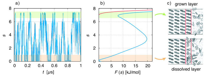
We describe a typical simulation taking as example the face at concentration = 1.5 nm-3. In Figure 5a, we show the time evolution of the CV used in WTMetaD, namely . During the simulation the system explores configurations in which the crystal layer is grown and dissolved. This should be compared to a standard MD simulation in which the system would remain for a much longer time in the dissolved state. From the simulation, the FES can be calculated using Equation (4) and is shown in Figure 5b (blue curve). As expected, shows two minima that correspond to the grown and dissolved states. To improve sampling a wall potential was imposed to prevent the growth of the full layer. The wall potential is shown as a red curve in Figure 5b (see SI for details). Representative simulation box snapshots for the two minima are shown in Figure 5c.
Although exhibits a free energy barrier, we decided to calculate the height of the barrier using a CV with a clear physical interpretation. For this reason, we reweighted[18] our results to calculate the FES as a function of , which approximates the number of crystalline molecules in the growing layer. In Figure 6, we show for all simulations, and the corresponding values of the are summarized in Table 1. For both concentrations, is substantially larger than and . Furthermore, is less sensitive to changes in concentration than and . For face , the free energy barriers differ between the two concentrations by 2.4 kJ/mol, while for faces and the free energy barriers differ by 5.0 kJ/mol.
It is important to note, that the sampled are strongly affected by the finite size effects [8]. In a small system, such as the one used in this work, the periodic boundary conditions of the simulation box induce an artificial stabilization of the emerging 2D nucleus on the surface of the crystal. This leads to an underestimation of the critical 2D nucleus size and as a consequence an underestimation of . It is however possible to obtain trends which are consistent with experiments as shown in the following. Also one has to point out that here we are interested in the relative behaviors and we expect that finite size effects cancel out approximately.
| = 1.2 nm-3 | 24.5 | 11.2 | 7.2 |
|---|---|---|---|
| = 1.5 nm-3 | 22.1 | 6.2 | 2.1 |
Now since we have the free energy barriers, we can compute the relative growth rates for each face and concentration. For the subsequent analysis we shall assume that all faces grow at the chosen supersaturations in the 2D nucleation regime. The perpendicular growth rate of a face growing by 2D nucleation can be written as [13, 42]
| (13) |
where is the interplanar spacing of the face and denotes the time to completely cover the crystal surface with a new layer of naphthalene molecules. Numerical values of are reported in the SI. depends on the nucleation rates and edge velocities of the emerging 2D nucleus. If we assume that nucleation is the rate limiting step, then we can approximate as the reciprocal of an Arrhenius type function [43, 42, 8]
| (14) |
where is a pre-exponential coefficient which is assumed to be the same for all faces.
According to Chernov [12, 44], the crystal morphology in a typical crystallization environment is determined by the crystal growth kinetics. The ratio of the perpendicular distances of faces and from the center of mass of the crystal, and , is proportional to the ratio of the growth rates of the two faces, and
| (15) |
With the ratios , the steady state crystal shape can be estimated for each supersaturation by solving a system of plane equations in the Cartesian coordinates[45].
For both concentrations, the predicted crystal shape is a wafer-thin rhombic prism, as shown in Figure 7 for = 1.2 nm-3. The blue colored large surface corresponds to the slow growing face, while the red colored thin surfaces correspond to the fast growing face. The very fast growing face is not present in the resulting steady state crystal shapes.
The activation energy barrier changes more rapidly with supersaturation for face than for face . Consequently, the ratio is about three times larger for = 1.5 nm-3 than for = 1.2 nm-3. Therefore the rhombic prism is about three times thinner for this higher concentration.
The simulation result at = 1.2 nm-3 is comparable with the experiment at high supersaturation reported by Lovette et al. in Reference [13]. Trends are captured well by the simulation, predicting that only faces and are present and that the face grows much faster in comparison to face .
3.2 Growth mechanisms

The biased simulations also allow to gain insight into the details of the growth mechanism. One should keep in mind that the simulations were performed with small surface areas exhibiting finite size effects. However, here again we are interested into trends which are expected to be the same for larger system sizes. Figure 8 shows the free energy surface, , as a function of the CV , that approximates the number of crystalline naphthalene molecules in the surface layer, and CV , i.e. the number of ethanol molecules residing in the surface layer.
We shall focus on the growth mechanism of face first (see for instance Figure 8a). The dissolved free energy minimum is strongly oriented along the axis. Therefore the system will experience fluctuations in the number of ethanol molecules in the surface before starting to form a crystalline 2D nucleus. Of course, the number of naphthalene molecules in the surface is anticorrelated to the number of naphthalene molecules in the same region. Indeed, we observe in the simulation trajectories that an amorphous agglomerate of naphthalene molecules appears before the onset of crystallinity. Only at a subsequent stage the system surmounts the barrier in the axis thus forming a crystalline 2D cluster that grows spontaneously.
From these observations we conclude that this face grows through a two step mechanism. The first step is characterized by the formation of an amorphous agglomerate of naphthalene molecules while during the second step the molecules order into the crystalline lattice. This mechanism can be observed for both concentrations, see Figures 8a and 8b. The minimum free energy path for the transformation is presented in red in the FES and is compatible with the description given above. The nudged elastic band method [46] was used for the calculation of the minimum free energy paths.
Now we turn to describe faces and that exhibit a growth mechanism different from the one of face . We analyze in particular Figure 8c. In this case the decrease in the number of ethanol molecules in the surface occurs concomitantly with the increase in the number of crystalline naphthalene molecules. This is confirmed by the atomistic trajectories in which we also observe that as soon as naphthalene molecules reach the surface, they simultaneously tend to orient according to the crystal lattice. This description is compatible with a one step mechanism different from the scenario in face . From the minimum free energy paths presented in red in Figure 8 the two different growth mechanisms can be clearly distinguished.
4 Conclusions
In this work, we have used molecular dynamics to predict the steady state crystal shape of naphthalene grown from ethanol solution at two different supersaturations. We calculated the free energy barriers for the growth of faces , , and using Well-Tempered Metadynamics. In order to mimic the experimental conditions the simulations were performed at constant supersaturation using the CMD algorithm [16]. From the free energy barriers we could estimate the relative growth rates and with them we predicted the steady state crystal shape. The resulting crystal shape is a wafer-thin rhombic prism, where only the and faces are present and the former face grows considerably slower. These predictions are in line with experiments.
We identified two different growth mechanisms. For the face, a two step nucleation was observed in which an amorphous agglomerate of naphthalene molecules has to form before the molecules arrange into the crystalline lattice. For the and faces the growth occurs with a concerted agglomeration and orientation of naphthalene molecules in the crystalline 2D nucleus.
The framework developed to enhance the growth of a single naphthalene crystal layer under constant supersaturation can be adapted to study the growth of more complicated organic molecules like APIs.
Conflicts of interest
There are no conflicts to declare.
Acknowledgements
Z.B. and M.M. are thankful for the financial support provided by Novartis Pharma AG, Lichtstrasse 35, 4056 Basel, Switzerland. P.M.P, T.K and M.P acknowledge support from the NCCR MARVEL funded by the Swiss National Science Foundation and from European Union Grant No. ERC-2014-AdG-670227/VARMET. Z.B. would like to thank Matteo Salvalaglio, Dan Mendels, Claudio Perego, and Riccardo Capelli for valuable discussions. Z.B. thanks GiovanniMaria Piccini for supplying the code used to calculate the minimum free energy paths presented in Figure 8. The computational resources were provided by ETH Zürich and the Swiss Center for Scientific Computing at the Euler Cluster.
References
- [1] Daniel Winn and Michael F. Doherty. Modeling crystal shapes of organic materials grown from solution. AIChE J., 46(7):1348–1367, 2000.
- [2] Jinjin Li, Carl J. Tilbury, Seung Ha Kim, and Michael F. Doherty. A design aid for crystal growth engineering. Prog. in Mat. Sci., 82:1–38, 2016.
- [3] X. Y. Llu, E. S. Boekt, W. J. Brlels, and P. Bennema. Prediction of crystal growth morphology based on structural analysis of the solid-fluid interface. Nature, 374:342–345, 1995.
- [4] Daniel Winn and Michael F. Doherty. Predicting the shape of organic crystals grown from polar solvents. Chem. Eng. Sci., 57(10):1805–1813, 2002.
- [5] Stefano Piana and Julian D. Gale. Understanding the barriers to crystal growth: Dynamical simulation of the dissolution and growth of urea from aqueous solution. J. Am. Chem. Soc., 127(6):1975–1982, 2005.
- [6] Stefano Piana, Franca Jones, and Julian D Gale. Assisted desolvation as a key kinetic step for crystal growth. J. Am. Chem. Soc., 128(41):13568–13574, 2006.
- [7] Jie Chen and Bernhardt L. Trout. Computer-aided solvent selection for improving the morphology of needle-like crystals: A case study of 2,6-dihydroxybenzoic acid. Cryst. Growth Des., 10(10):4379–4388, 2010.
- [8] Matteo Salvalaglio, Thomas Vetter, Federico Giberti, Marco Mazzotti, and Michele Parrinello. Uncovering molecular details of urea crystal growth in the presence of additives. J. Am. Chem. Soc., 134(41):17221–17233, 2012.
- [9] Tarak Karmakar, Pablo M. Piaggi, Claudio Perego, and Michele Parrinello. A cannibalistic approach to grand canonical crystal growth. J. Chem. Theory Comput., 14(5):2678–2683, 2018.
- [10] Dandan Han, Tarak Karmakar, Zoran Bjelobrk, Junbo Gong, and Michele Parrinello. Solvent-mediated morphology selection of the active pharmaceutical ingredient isoniazid: Experimental and simulation studies. Chem. Eng. Sci., page in press, 2019.
- [11] Matteo Salvalaglio, Thomas Vetter, Marco Mazzotti, and Michele Parrinello. Controlling and predicting crystal shapes: The case of urea. Angew. Chem. Int. Ed., 52(50):13369–13372, 2013.
- [12] A. A. Chernov. Kinetics of the growth forms of crystals. Sov. Phys. Crystallography, 7(6):728–730, 1962.
- [13] Michael A. Lovette and Michael F. Doherty. Predictive modeling of supersaturation-dependent crystal shapes. Cryst. Growth Des., 12(2):656–669, 2012.
- [14] R. F. P. Grimbergen, M. F. Reedijk, H. Meekes, and P. Bennema. Growth behavior of crystal faces containing symmetry-related connected nets: A case study of naphthalene and anthracene. J. Phys. Chem. B, 102(15):2646–2653, 1998.
- [15] Alessandro Barducci, Giovanni Bussi, and Michele Parrinello. Well-tempered metadynamics: A smoothly converging and tunable free-energy method. Phys. Rev. Lett., 100(2):020603, 2008.
- [16] C. Perego, M. Salvalaglio, and M. Parrinello. Molecular dynamics simulations of solutions at constant chemical potential. J. Chem. Phys., 142(14):144113, 2015.
- [17] Omar Valsson, Pratyush Tiwary, and Michele Parrinello. Enhancing important fluctuations: Rare events and metadynamics from a conceptual viewpoint. Annu. Rev. Phys. Chem., 67:159–184, 2016.
- [18] Pratyush Tiwary and Michele Parrinello. A time-independent free energy estimator for metadynamics. J. Phys. Chem. B, 119(3):736–742, 2015.
- [19] Erik E. Santiso and Bernhardt L. Trout. A general set of order parameters for molecular crystals. J. Chem. Phys., 134(6):064109, 2011.
- [20] Cristian Micheletti, Alessandro Laio, and Michele Parrinello. Reconstructing the density of states by history-dependent metadynamics. Phys. Rev. Lett., 92(17):170601, 2004.
- [21] Yanier Crespo, Fabrizio Marinelli, Fabio Pietrucci, and Alessandro Laio. Metadynamics convergence law in a multidimensional system. Phys. Rev. E, 81(5):055701, 2010.
- [22] Davide Branduardi, Giovanni Bussi, and Michele Parrinello. Metadynamics with adaptive gaussians. J. Chem. Theory Comput., 8(7):2247–2254, 2012.
- [23] Junmei Wang, Romain M. Wolf, James W. Caldwell, Peter A. Kollman, and David A. Case. Development and testing of a general amber force field. J. Comput. Chem., 25(9):1157–1174, 2004.
- [24] Junmei Wang, Wei Wang, Peter A. Kollman, and David A. Case. Automatic atom type and bond type perception in molecular mechanical calculations. J. Mol. Graph. Model., 25(2):247–260, 2006.
- [25] Christopher I. Bayly, Piotr Cieplak, Wendy Cornell, and Peter A. Kollman. A well-behaved electrostatic potential based method using charge restraints for deriving atomic charges: the resp model. J. Phys. Chem., 97(40):10269–10280, 1993.
- [26] M. J. Frisch, G. W. Trucks, H. B. Schlegel, G. E. Scuseria, M. A. Robb, J. R. Cheeseman, G. Scalmani, V. Barone, B. Mennucci, G. A. Petersson, H. Nakatsuji, M. Caricato, X. Li, H. P. Hratchian, A. F. Izmaylov, J. Bloino, G. Zheng, J. L. Sonnenberg, M. Hada, M. Ehara, K. Toyota, R. Fukuda, J. Hasegawa, M. Ishida, T. Nakajima, Y. Honda, O. Kitao, H. Nakai, T. Vreven, J. A. Montgomery, J. E. Peralta, F. Ogliaro, M. Bearpark, J. J. Heyd, E. Brothers, K. N. Kudin, V. N. Staroverov, R. Kobayashi, J. Normand, K. Raghavachari, A. Rendell, J. C. Burant, S. S. Iyengar, J. Tomasi, M. Cossi, N. Rega, J. M. Millam, M. Klene, J. E. Knox, J. B. Cross, V. Bakken, C. Adamo, J. Jaramillo, R. Gomperts, R. E. Stratmann, O. Yazyev, A. J. Austin, R. Cammi, C. Pomelli, J. W. Ochterski, R. L. Martin, K. Morokuma, V. G. Zakrzewski, G. A. Voth, P. Salvador, J. J. Dannenberg, S. Dapprich, A. D. Daniels, Farkas, J. B. Foresman, J. V. Ortiz, J. Cioslowski, and D. J. Fox. Gaussian 09, revision b.01, 2009.
- [27] Alan W. Sousa da Silva and Wim F. Vranken. Acpype - antechamber python parser interface. BMC Research Notes, 5:367, 2012.
- [28] D. W. J. Cruickshank. A detailed refinement of the crystal and molecular structure of naphthalene. Acta Cryst., 10:504–508, 1957.
- [29] D. H. Andrews, George Lynn, and John Johnston. The heat capacities and heat of crystallization of some isomeric aromatic compounds. J. Am. Chem. Soc., 48(5):1274–1287, 1926.
- [30] David van der Spoel, Paul J. van Maaren, and Carl Caleman. Gromacs molecule & liquid database. Bioinformatics, 28(5):752–753, 2012.
- [31] H. J. C. Berendsen, D. van der Spoel, and R. van Drunen. Gromacs: A message-passing parallel molecular dynamics implementation. Comput. Phys. Commun., 91(1):43–56, 1995.
- [32] Erik Lindahl, Berk Hess, and David van der Spoel. Gromacs 3.0: a package for molecular simulation and trajectory analysis. J. Mol. Model., 7(8):306–317, 2001.
- [33] David van der Spoel, Erik Lindahl, Berk Hess, Gerrit Groenhof, Alan E. Mark, and Herman J. C. Berendsen. Gromacs: Fast, flexible, and free. J. Comput. Chem., 26(16):1701–1718, 2005.
- [34] Berk Hess, Carsten Kutzner, David van der Spoel, and Erik Lindahl. Gromacs 4: Algorithms for highly efficient, load-balanced, and scalable molecular simulation. J. Chem. Theory Comput., 4(3):435–447, 2008.
- [35] Mark James Abraham, Teemu Murtola, Roland Schulz, Szilard Pall, Jeremy C. Smith, Berk Hess, and Erik Lindahl. Gromacs: High performance molecular simulations through multi-level parallelism from laptops to supercomputers. SoftwareX, 1–2:19–25, 2015.
- [36] Gareth A. Tribello, Massimiliano Bonomi, Davide Branduardi, Carlo Camilloni, and Giovanni Bussi. Plumed 2: New feathers for an old bird. Comput. Phys. Commun., 182(2):604–613, 2014.
- [37] Giovanni Bussi, Tatyana Zykova-Timan, and Michele Parrinello. Isothermal-isobaric molecular dynamics using stochastic velocity rescaling. J. Chem. Phys., 130(7):074101, 2009.
- [38] Tom Darden, Darrin York, and Lee Pedersen. Particle mesh ewald: An n log(n) method for ewald sums in large systems. J. Chem. Phys., 98(12):10089–10092, 1993.
- [39] Berk Hess. P-lincs: A parallel linear constraint solver for molecular simulation. J. Chem. Theory Comput., 4(1):116–122, 2008.
- [40] M. Parrinello and A. Rahman. Polymorphic transitions in single crystals: A new molecular dynamics method. J. Appl. Phys., 52(12):7182–7190, 1981.
- [41] William Humphrey, Andrew Dalke, and Klaus Schulten. Vmd: Visual molecular dynamics. J. Mol. Graph., 14(1):33–38, 1996.
- [42] Xiang-Yang Liu and P. Bennema. Theoretical consideration of the growth morphology of crystals. Phys. Rev. B, 53(5):2314–2325, 1996.
- [43] Svante Arrhenius. über die reaktionsgeschwindigkeit bei der inversion von rohrzucker durch säuren. Z. Phys. Chem., 4(1):226–248, 1889.
- [44] Michael A. Lovette, Andrea Robben Browning, Derek W. Griffin, Jacob P. Sizemore, Ryan C. Snyder, and Michael F. Doherty. Crystal shape engineering. Ind. Eng. Chem. Res., 47(24):9812–9833, 2008.
- [45] Yongchun Zhang, Jacob P. Sizemore, and Michael F. Doherty. Shape evolution of 3-dimensional faceted crystals. AIChE J., 52(5):1906–1915, 2006.
- [46] Graeme Henkelman and Hannes Jonsson. Improved tangent estimate in the nudged elastic band method for finding minimum energy paths and saddle points. J. Chem. Phys., 113(22):9978–9985, 2000.
Supplementary information
Parameters used for biased simulations
Parameters of the surface layer crystallinity CV, , and biased CV, , used in the simulations are summarized in Table 2. The Well-Tempered Metadynamics parameters are summarized in Table 3, where is the bin size of the grid on which the positions of the Gaussian potentials are discretized.
| [rad] | 0.0000 | 0.0000 | 0.0000 |
|---|---|---|---|
| [rad] | 0.4400 | 0.4400 | 0.4400 |
| [rad] | 2.7016 | 2.7016 | 2.7016 |
| [rad] | 3.1416 | 3.1416 | 3.1416 |
| [rad] | 0.15 | 0.15 | 0.15 |
| [rad] | 0.15 | 0.15 | 0.15 |
| [rad] | 0.15 | 0.15 | 0.15 |
| [rad] | 0.15 | 0.15 | 0.15 |
| [nm] | 0.65 | 0.90 | 0.90 |
| [-] | 4 | 4 | 4 |
| [-] | 15 | 15 | 15 |
| [-] | 0.5884 | 0.5958 | 0.5958 |
| [-] | 0.6304 | 0.6229 | 0.6229 |
| [-] | 2000 | 2000 | 2000 |
| [-] | 2000 | 2000 | 2000 |
| [-] | 0.7 | 0.5 | 0.5 |
| [kJ/mol] | 0.8 | 0.5 | 0.5 |
|---|---|---|---|
| [-] | 0.7 | 0.4 | 0.4 |
| [K] | 12 | 10 | 8 |
| [ps] | 1 | 1 | 1 |
| [-] | 0.14 | 0.08 | 0.08 |
Naphthalene force field
| atom | GAFF | RESP | mass | |||
|---|---|---|---|---|---|---|
| name | atom type | charge [e] | [g/mol] | [nm] | [nm] | [nm] |
| C1 | ca | -0.116476 | 12.010 | 0.000 | 0.244 | -0.071 |
| C2 | ca | -0.116476 | 12.010 | 0.000 | 0.244 | 0.071 |
| C3 | ca | -0.264483 | 12.010 | 0.000 | 0.125 | 0.140 |
| C4 | ca | -0.264483 | 12.010 | 0.000 | -0.125 | 0.140 |
| C5 | ca | -0.116476 | 12.010 | 0.000 | -0.244 | 0.071 |
| C6 | ca | -0.264483 | 12.010 | 0.000 | 0.125 | -0.140 |
| C7 | ca | -0.116476 | 12.010 | 0.000 | -0.244 | -0.071 |
| C8 | ca | 0.216029 | 12.010 | 0.000 | 0.000 | 0.072 |
| C9 | ca | 0.216029 | 12.010 | 0.000 | 0.000 | -0.072 |
| C10 | ca | -0.264483 | 12.010 | 0.000 | -0.125 | -0.140 |
| H1 | ha | 0.127069 | 1.008 | 0.000 | 0.338 | -0.125 |
| H2 | ha | 0.127069 | 1.008 | 0.000 | 0.338 | 0.125 |
| H3 | ha | 0.145875 | 1.008 | 0.000 | 0.124 | -0.249 |
| H4 | ha | 0.145875 | 1.008 | 0.000 | 0.124 | 0.249 |
| H5 | ha | 0.145875 | 1.008 | 0.000 | -0.124 | 0.249 |
| H6 | ha | 0.127069 | 1.008 | 0.000 | -0.338 | 0.125 |
| H7 | ha | 0.127069 | 1.008 | 0.000 | -0.338 | -0.125 |
| H8 | ha | 0.145875 | 1.008 | 0.000 | -0.124 | -0.249 |
The general AMBER force field (GAFF) [23] parameters of naphthalene obtained by the procedure described in the main text are listed in Table 4 (check Figure 9 for the numbering of the atoms).
To estimate how well the naphthalene GAFF reproduces the experimental crystal structure, simulations of a nm3 crystal were performed under conditions with anisotropic pressure coupling [40] at 1 bar and 300 K. Figure 10 shows the radial distribution function, , and the PDFs of the vector angles, and . The red lines were computed from XRD measurement data [28] and the three blue lines are simulation results at times 3 ns, 6 ns, and 9 ns. The center of mass of carbon atoms 8 and 9 were defined as molecule center and the vector angle definitions are shown in Figure 9. Simulation results for , , and show all satisfactory agreement with the XRD data.
The melting temperature of the naphthalene GAFF was estimated by simulation runs of a roughly 333 nm3 crystal slab exposing the face to a liquid naphthalene phase around twice the size of the crystal. Simulations were performed at different temperatures under conditions with the velocity rescale thermostat [37] and semi-isotropic Parrinello-Rahman barostat [40] ( and coupled, decoupled) at 1 bar. Growth of the crystal slab was observed at temperatures below 330 K, while at temperatures at and above 330 K the crystal slab was melting. The trajectories of the system crystallinity, , for the different temperatures are presented in Figure 11. The CV takes all solute molecules of the system into account and is reported in Reference [8]. The simulated melting temperature of K lies sufficiently close to the experimental one at 352 - 354 K [29].
To obtain the initial configurations for both the crystallographic structure comparison and for the melting temperature, the equilibration procedure was used which is described in the following section. All MD simulation parameters which were utilized for the simulations above and are not explicitly mentioned, are described in the main text.
Simulation setup equilibration
All equilibration steps were performed with Gromacs 2016.5 [35] using the velocity rescaling thermostat [37], periodic boundary conditions, the particle mesh Ewald approach [38] for the electrostatic interactions, and the LINCS algorithm [39, 34] to constrain the covalent bonds involving hydrogens. The non-bonded cutoff was set to 1 nm.
For each crystal face, the following procedure was performed to obtain initial configurations for the three slowest growing naphthalene crystal faces, , , and [14]. A seed crystal was constructed from the XRD data [28] with the face of interest perpendicular to the -axis. The crystal system was first minimized with the conjugate gradient algorithm with a tolerance on the maximum force of 50 kJ mol-1 nm-1, and subsequently equilibrated under conditions for 1 ns, at 280 K and an integration time step of 0.5 fs. A temperature of 280 K was chosen to match the temperature of the experiments reported by Lovette et al. [13].
In a second step, the system was equilibrated for 10 ns under conditions with the anisotropic Parrinello-Rahman barostat [40] at 1 bar, 280 K, and with the same integration time step of 0.5 fs. From the equilibration (while not considering the first 1 ns), the frame with box size values , , and the ratio , closest to the average values, was considered. The averaged crystal configuration was then submerged in the solution by extending the box length to more than four times the crystal length in the -direction and filling the box with naphthalene and ethanol molecules using the genbox utility of Gromacs [34].
For the system containing the crystal as well as the solution, the same minimization and equilibration steps were performed. Although for the equilibration, the box expansion was only allowed in the -direction, keeping and constant. The simulation frame with box length closest to the average one (again omitting the first 1 ns) was picked as initial configuration for the last equilibration step involving the CMD algorithm [16].
To obtain the final initial configuration which holds the targeted concentrations in both control regions, the system had to undergo an equilibration procedure, in which the average concentration profile along the -axis becomes static. A simulation of 25 ns ensured to reach an adequate convergence. The last frame of the concentration profile equilibration for each face and supersaturation was used for the simulations. The numerical parameter values of the CMD algorithm are shown in Table 5.
The number of molecules and simulation box lengths used for the biased simulations are presented in Table 6.
| [kJ/mol] | [-] | [-] | [-] | [-] | [-] |
|---|---|---|---|---|---|
| 1500 | 0.04 | 0.11 | 0.26 | 0.33 | 1/120 |
| face | number of molecules [-] | box lengths [nm] | |||
|---|---|---|---|---|---|
| naphthalene | ethanol | ||||
| 380 | 1053 | 2.975 | 3.577 | 16.560 | |
| 360 | 951 | 3.035 | 3.172 | 16.936 | |
| 360 | 951 | 3.287 | 2.985 | 16.655 | |
CMD concentration profiles
Parameters used in the CMD algorithm are shown in Table 5. And the corresponding concentration profiles for all six biased simulation runs (each performed for 1 s) are shown in Figure 12. The crystal surface was biased on the right side of the crystal shown in the middle of each graph, while the surface on the left was not biased at all. The target concentrations in both control regions were met with satisfactory accuracy.
Solubility estimation
To our knowledge, no simple algorithm exists for computing the exact solubility of naphthalene in ethanol at the given conditions. However it is possible to estimate the limits within the solubility is located by the use of the CMD algorithm and long enough simulation runs. Figure 13 shows the system crystallinity CV, , trajectories for different runs of the three simulation series, each under different concentrations, = 0.6 nm-3, = 0.8 nm-3, and = 1.0 nm-3. For each concentration series the total time of all simulation runs sums up to 7.5 s. In case of = 0.6 nm-3, six dissolution events while no growth events were observed. For = 0.8 nm-3 two dissolution and two growth events were observed. While for = 1.0 nm-3, no dissolution, however five growth events were observed. The solubility is therefore estimated to reside around = 0.8 nm-3.
Constraint of seed crystal movement
For the biased simulations, the center of mass of the two most inner layers of each seed crystal was constrained in its movement along the axis with a harmonic potential. The force constant was set to 1500 kJ/mol for all three faces.
Use of wall potentials for biased simulations
A lower and an upper wall potential were set to constrain the sampling to the relevant region:
| (16) |
The lower wall potential inhibits from getting stuck at the value of zero, causing the biased simulation to crash. While the upper wall plays the important role of not letting the system completing the biased layer, since it would increase the convergence time significantly. As already indicated by Piana et al. [5], the removal of solvent molecules from the remaining surface gap of the almost fully grown layer corresponds to a slow process. The upper wall potential prevents the system from reaching the CV space where the surface gap would emerge.
| [nm-3] | 1.2 | 1.5 | 1.2 | 1.5 | 1.2 | 1.5 |
|---|---|---|---|---|---|---|
| [kJ/mol] | 75 | 75 | 50 | 50 | 50 | 50 |
| [-] | 0.07 | 0.07 | 0.07 | 0.07 | 0.07 | 0.07 |
| [kJ/mol] | 10 | 10 | 25 | 25 | 10 | 25 |
| [-] | 7.0 | 7.0 | 3.5 | 3.5 | 3.5 | 3.0 |
Surface layer crystallinity trajectories
The trajectories of the surface layer crystallinity CV, , of the biased simulations are shown in Figure 14. The first 200 ns of were not considered in the reweighting procedure [18] for all reweighted plots reported in the main text.
Numerical values for the interplanar spacing
Numerical values for the interplanar spacing, , used for the calculation of the steady state crystal shape can be found in Table 8. The values were obtained from simulations of a crystal of size nm3 by using the anisotropic Parrinello-Rahman barostat [40] and taking the average lengths of . The simulations were performed for 10 ns each.
| [nm] | 0.929 | 0.451 | 0.410 |
|---|