Estimation of Linear Motion in Dense Crowd Videos using Langevin Model

^∗Shreetam Behera^a, Debi Prosad Dogra^a, Malay Kumar Bandyopadhyay^b and Partha Pratim Roy^c Address: School of Electrical Science,^a
Indian Institute of Technology Bhubaneswar, Bhubaneswar-752050, India^a
School of Basic Sciences,^b
Indian Institute of Technology Bhubaneswar, Bhubaneswar-752050, India^b
Department of Computer Science and Engineering^c,
Indian Institute of Technology Roorkee, Roorkee-247667, India^c
Email: sb46@iitbbs.ac.in^a, dpdogra@iitbbs.ac.in^a, malay@iitbbs.ac.in^b, proy.fcs@iitr.ac.in^c Email: sb46@iitbbs.ac.in

Abstract

Crowd gatherings at social and cultural events are increasing in leaps and bounds with the increase in population. Surveillance through computer vision and expert decision making systems can help to understand the crowd phenomena at large gatherings. Understanding crowd phenomena can be helpful in early identification of unwanted incidents and their prevention. Motion flow is one of the important crowd phenomena that can be instrumental in describing the crowd behavior. Flows can be useful in understanding instabilities in the crowd. However, extracting motion flows is a challenging task due to randomness in crowd movement and limitations of the sensing device. Moreover, low-level features such as optical flow can be misleading if the randomness is high. In this paper, we propose a new model based on Langevin equation to analyze the linear dominant flows in videos of densely crowded scenarios. We assume a force model with three components, namely external force, confinement/drift force, and disturbance force. These forces are found to be sufficient to describe the linear or near-linear motion in dense crowd videos. The method is significantly faster as compared to existing popular crowd segmentation methods. The evaluation of the proposed model has been carried out on publicly available datasets as well as using our dataset. It has been observed that the proposed method is able to estimate and segment the linear flows in the dense crowd with better accuracy as compared to state-of-the-art techniques with substantial decrease in the computational overhead.

Keywords:

Crowd Flow Segmentation, Crowd Dynamics, Visual Surveillance, Langevin Equation

1 Introduction

Recent advancement in computer vision-based crowd surveillance has drawn interests of the researchers and law enforcing agencies across the world. Automatic visual surveillance through expert decision making systems often results in efficient crowd monitoring and management with higher accuracy and better information fusion. Moreover, such intelligent systems can reduce human efforts leading to less errors in estimation. Expert systems guided automatic visual surveillance frameworks can promptly indicate unusual behavior or activity in crowd. Therefore, precautionary measures can be taken in order to avoid undesirable incidents. Such systems can also be used to understand human behavior of the people in crowded situations. However, majority of existing systems find it hard to handle dense crowds such as religious festivals, social and political gatherings because of the complexity of the problem in terms of functionality and time (Junior et al. 2010). Computer vision research community tend to adopt machine vision-based algorithms in the above situations (Junior et al. 2010; Yogameena and Nagananthini 2017).

1.1 Related Work

Flow detection and segmentation are key to develop automatic crowd monitoring systems. Existing research work on crowd flow segmentation are either physics and particle dynamics-based or standard computer vision guided techniques as mentioned in (Zhang et al. 2018).

1.1.1 Physics or Particle Dynamics-based Methods

In case of physics-based or particle dynamics-based methods, typical fluid-flow model or freely moving particles on air may not be directly applied on crowd. For example, Langevin theory of Brownian motion may not be directly applied on crowd dynamics. However, such physics-based models can be adopted with context imposed restrictions. For example, correlating the actual forces in dense crowded situations with particle dynamics can be interesting. Such models have started to emerge off late (Zhang et al. 2018). Ali et al. (Ali and Shah 2007) have used Lagrange particle dynamics to segment high density crowd flows. The same framework has also been used for detecting instabilities in crowd flows. Zhang et al. in (Zhong et al. 2008) have used Markov Random Field to define crowd energy upon which wavelet analysis has been performed to detect abnormal behaviors. However, the method is not independent of background and it is sensitive to video shaking. The authors in (Ali and Shah 2008) have used a scene-structure-based force model to detect individuals in high-density crowd by analyzing its static, dynamic, and boundary floor fields. The algorithm is highly computation intensive. Mehran et al. (Mehran et al. 2010) have used streaklines for crowd flow analysis. They have used social force graph technique and streaklines to analyze the flow. The authors of (Ji et al. 2017) have proposed a method based on social force model to detect crowd anomaly at pixel and block levels. In (Wu et al. 2017), the authors perform analysis of the crowd based on a bilinear interaction of curl and divergence of the flows. In (Ullah et al. 2017), a density independent hydrodynamics model (DIHM) for coherency detection in crowded scenes, has been proposed. The method has the capability to handle changing density over time. The method doesn’t perform finer-level crowd flow segmentation. A spatio-temporal driving force model has been proposed in (Li and Chellappa 2010) to perform group segmentation in crowded scenarios. However, the model is not view variant and it needs to learn for different views with different parameter settings. In (Chen et al. 2011), the authors have presented an adaptive human motion analysis and prediction method for understanding the motion patterns in crowds. Solmaz et al. in (Solmaz et al. 2012) have proposed a method to identify multiple crowd behaviors through stability analysis for dynamical systems avoiding object detection, tracking, or training. Their method cannot capture the randomness in a crowd. In (Lin et al. 2016), coherent regions in a crowded scene is detected based on thermal diffusion process and time-series clustering. The coherency is lost as the method merges both the motion and non-motion regions together over time. The agent-based method proposed in (Kountouriotis et al. 2014) can model crowd behavior based on group dynamics and agent-based personality traits. Though their method performs reasonably well in real-time scenario, but its performance ceases with increase in the number of agents. In (Zhou et al. 2015), Zhou et al. have proposed a new mixture model of dynamic pedestrian-Agents (MDA) to learn the collective behavioral patterns of pedestrians in crowded scenes. However, it is unclear that how their method can handle varying density. In (Su et al. 2013), the authors have proposed a spatio-temporal viscous fluid field to recognize the large-scale crowd behavior from appearance and driven factor perspectives. An application of real-time monitoring of crowd density at Puri Rath Yatra, combined with modeling evacuation scenarios using agent-based simulation has been proposed in (Basak and Gupta 2017). The technique is useful in predicting scenarios in emergency situations even though the technique is computationally expensive.

1.1.2 Computer Vision-based Methods

Conventional computer vision-based methods like optical flow-based methods have been instrumental in flow segmentation. The method proposed in
(Cheriyadat and Radke 2008) finds dominant motions of crowd by clustering low-level feature point tracks in videos. Wu et al. (Wu et al. 2009a) have presented a region growing segmentation scheme based on the translational domain for segmenting crowd flows. The method fails if the translational flow is not local. Santoro et al. (Santoro et al. 2010) have used Lucas-Kanade Tracker along with the density-based clustering for analysis of crowd motion. In the last step, a crowd tracker has been applied in each frame of the video. The authors claims their method can detect and track crowd with various shapes. However, the calculations are based on 2D coordinates of the motion point. Thus, the distance calculation between the motion points is not accurate. Moreover, the time complexity increases with the increase in motion points. In (Wu et al. 2009b), the authors have proposed a new framework for crowd movement analysis. The crowd flow segmentation is performed using optical flow field. An interpolation method based on Delaunay Triangulation has been used to estimate the smooth optical flow field in a robust way. Motion regions are then clustered and a shape derivative technique is combined with a region growing scheme in order to segment a crowd. However, the method cannot detect all motion regions in a typical crowd. The authors in (Lu et al. 2017) have proposed a trajectory clustering-based method to understand crowd motion patterns. The method in (Nasir et al. 2014) aims to generate accurate sequence waypoints for the pedestrian walking path by analyzing videos in closed environments only. The authors in (Anwar et al. 2012) have developed an anomaly detection method to analyze anomalous events. However, the proposed method works at microscopic level. An Interval-Based Spatio-Temporal Model (IBSTM) have been proposed in (Kardas and Cicekli 2017) in order to detect untoward events in a video. However, the proposed method is a microscopic event model that cannot deal with macroscopic events such as crowd flow. The method proposed in (Walia et al. 2017) uses a multi-stage tracker for precise localization of targets. However, this model is a microscopic model aimed at individual humans only. The authors in (Fernández-Caballero et al. 2012) have proposed a finite state machines-based technique for human activity monitoring in a closed scene. The method needs to have prior information about source and destination points. The method described in (Zhou et al. 2014) segments the motion flow in sparse crowds in terms of collectiveness. Fradi et al. (Fradi et al. 2017) have proposed local descriptors which provide semantic information and interactive sparse crowd behaviors. However, it is not clear how the method handles dense crowd.

Traditional computer vision algorithms amalgamated with machine learning techniques have also been used for performing crowd flow segmentation in videos. Cao et al. (Cao et al. 2015) have performed large scale crowd analysis using Convolutional Neural Networks (CNN). The authors have combined CNN guided classification with regression to get accurate results. However, a large database with proper labeling must be available for such a method to be successful. The authors in (Zhou et al. 2016) have proposed a spatio-temporal CNN for crowd anomaly detection. In (Kruthiventi and Babu 2015), crowd flow analysis is performed using Conditional Random Field. However, the method is incapable to handle intersecting flows. Deep learning-based optical flow schemes are also proposed in (Dosovitskiy et al. 2015) and (Ilg et al. 2017) to predict optical flow of consecutive frames based on Convolution Neural Networks. But, they do not address the dynamics of typical crowded scenarios. The methods proposed in (Shao et al. 2015) and (Long et al. 2015) are based on deep learning techniques for scene understanding and semantic segmentation. However, these methods are unable to describe the dynamics of the crowd. The authors of (Chaker et al. 2017) have proposed an unsupervised approach for crowd scene anomaly detection based on the social network model. In the paper (Wu et al. 2018), collective density clustering is performed for detection of coherent crowd regions. However, the method is dependent on stability and accuracy of the tracking algorithm. In (Direkoglu et al. 2017), the angle difference between optical flow vectors, has been used as a feature, fed to Support Vector Machine (SVM) for detecting abnormality in crowd. The authors in (Yuan et al. 2016) have proposed a sparse representation method for crowd anomaly detection. The work presented in (Chan and Vasconcelos 2008) and (Ma et al. 2009) are based on dynamic mixture model of textures and expected-maximization (EM) algorithm. Such methods can segment motion in traffic and crowd videos. However, the authors have not provided any evidence on how it addresses crowd in terms of varying density.

From the aforementioned work, we have made the following observations:

1.

The methods similar to (Santoro et al. 2010) are restricted to be applicable for low and medium density crowd. These methods lack robustness in handling densely crowded scenarios.
2.

Though the physics-based (Chaker et al. 2017) and particle-dynamics-based (Ali and Shah 2007) models partially address the issues in densely crowded scenarios, they are complex in functionality and often leads to increased execution time. Moreover, such methods lack simplicity from the point of implementation.
3.

It has also been understood that, none of the existing methods such as (Ali and Shah 2007) or (Ullah et al. 2017) address the movement as random particles in the fluid. This has been one of the key motivations behind the idea presented in this paper.

1.2 Contributions

Following research contributions have been made to mitigate the aforementioned limitations:

1.

We propose a fast computational model to understand the dense crowd flow in videos using Langevin theory of Brownian particles in fluid.
2.

Using the aforementioned model, we propose an algorithm that can segment linear and near-linear flows of dense crowd movements in videos with the help of a context adaptive force model.

The rest of the paper is organized as follows. The foundation of Langevin equation is explained in Section 2. In Section 3, we explain how Langevin equation can be adopted for designing expert decision making system to understand crowd flow through segmentation. The results are presented in Section 4 using public datasets as well as using our video dataset. In Section 5, we have concluded the paper with possible future directions.

2 Background and Foundation

Langevin equation is perhaps the simplest way to describe the dynamics of non-equilibrium systems. It is a stochastic differential equation introduced first to describe the motion of a particle in fluid as mentioned in (Langevin 1908; Coffey and Kalmykov 2004). Since the motion of a particle is random, it cannot be described only using Newton’s force. In order to estimate the random and fluctuating motions of the particle, the basic Newtonian force is added with two additional force components: frictional force and random force.

Figure 1: Pictorial representation of interaction of a Brownian particle with different forces in a fluid.

Figure 2: Representation of particles in motion in 2D space, grouped with similar orientations, experiencing drift and confinement forces along

x

and

y

-axes, respectively.

Consider the 1D motion of a particle of mass $m$ as shown in Fig.1. According to Newton’s second law of motion, the motion of the particle is described using (1),

\frac{\text{d}v(t)}{\text{d}t}=F(t)

(1)

where $m$ is the mass of the particle, $v(t)$ is the velocity of the particle at time $t$ and $F(t)$ is the instantaneous force exerted on the particle at time $t$ .

The instantaneous force $F(t)$ as represented in (2), acting on a particle, is originated from the impact received from the surrounding fluid molecules. Langevin suggested that the force $F(t)$ can be written as a sum of two components. The first part is an $averaged-out$ component which basically represents the viscous drag, $-\gamma v(t)$ , where $\gamma$ is the frictional coefficient. In general, this frictional force is assumed to be proportional to the velocity of the particle. The second component of this instantaneous force $F(t)$ is a rapidly fluctuating part $\xi(t)$ which arises due to random density fluctuations in the fluid.

m\frac{\text{d}v(t)}{\text{d}t}=-\gamma v(t)+\xi(t)

(2)

The random force $\xi(t)$ averages out to be zero over long intervals as mentioned in (3). The second moment is actually relating the fluctuating force with the viscous drag or dissipative force $g$ , which is related to $\gamma$ as mentioned in (4),

\langle\xi(t)\rangle_{\xi}=0,~\langle\xi(t_{1})\xi(t_{2})\rangle_{\xi}=g\delta(t_{1}-t_{2})

(3)

where $\langle\xi(t)\rangle_{\xi}$ represents an average value considered with respect to the distribution of the realizations of the variable $\xi(t)$ ,

\texttt{g}=2\xi K_{B}T

(4)

and $g$ is the measure of strength of the fluctuation force, $K_{B}$ is Boltzmann’s constant, $T$ is the temperature, and $\delta$ is the delta function.

3 Proposed Crowd Flow Segmentation Method

The proposed crowd segmentation method using Langevin equation is discussed here. For a given video sequence, over a window of size $W$ , the keypoints are extracted and propagated to the proposed model as illustrated in Fig.3. Inside a typical window, this partial flow information is passed on to the proposed model where flow segmentation is carried out over the remaining frames of the window. Windowing ensures re-initialization of the process at regular intervals, which tracks the flow changes in the frames in temporal domain.

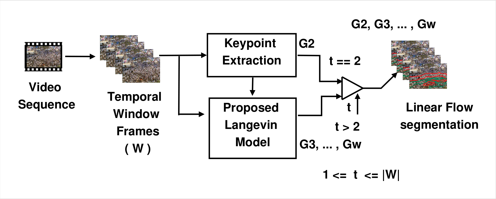
Refer to caption — Figure 3: Block diagram representation of the proposed crowd flow segmentation scheme. Over a temporal window $W$ , the first two frames are used for keypoint extraction to generate segmented map $G_{2}$ consisting of grouped keypoints and the subsequent frames are used for Langevin guided flow segmentation to generate $|W|-1$ segmented maps.

3.1 Keypoint Extraction

Dense optical flow using Farneback’s method as described in (Farnebäck 2003) has been estimated on first two down-scaled frames of $W$ . The flow vectors obtained are used to compute magnitude and orientation maps using equations (5) and (6), respectively. The orientation map is quantized into eight bins using a magnitude threshold within $[0,2\pi]$ . The envelope joining all the bin peaks forms a quantization curve.

v=\sqrt{|v_{x}|^{2}+|v_{y}|^{2}}

(5)

\theta=\arctan{(|v_{y}|/|v_{x}|)}

(6)

Using a standard peak detection algorithm upon this quantization curve, the peaks are detected. Keypoints corresponding to these peaks are retained and others are discarded. In the next step, grouping of retained keypoints is performed. Mainly, two factors are considered for grouping: orientation and spatial connectivity. The keypoints surrounding the considered keypoint are in a group if their quantized orientations are equal and they lie within a $3$ x $3$ neighborhood of the considered keypoint. The last condition accounts for the spatial connectivity of the considered keypoint with its neighboring keypoints. These grouped keypoints are assumed as initial segregated structured flows and are fed to Langevin-based model for the temporal flow segmentation for the remaining frames within the window. The entire process is illustrated in Fig.4.

3.2 Langevin Equation-guided Flow Segmentation

3.2.1 Formulation of Langevin Equation-based Force Model

The dense crowd can be considered analogous to particles moving in the fluid. After careful visual observation of several real-live crowd movement videos, we have realized that, structured crowd usually move together in groups of similar orientations as shown in Fig.2. In such cases, it is possible to approximate the motion with the help of Langevin theory. We have assumed that the force is acting on these groups instead of individual particle. Thus, the resultant force can be reconstructed as combination of various forces acting upon and within the group as represented in (7).

{F_{inertial}=~F_{external}+F_{drift/confine}+F_{disturbance}}

(7)

The resultant force as mentioned in (7) is constituted with external forces arising due to the motion of the group in the surrounding ( $F_{external}$ ), the drift forces that may cause the particle to drift along with the group in a particular direction or the confinement forces that confines the particles to stay within the group i.e. ( $F_{drift/confine}$ ), and disturbances due to the noise in the group ( $F_{disturbance}$ ).

For example, if we assume the movement of particles of the group along $x$ -axis as depicted in Fig. 2, inertial force on a particle along $x$ -axis can be represented as (8),

m\frac{d^{2}x}{dt^{2}}\ =-\gamma_{x}\frac{dx}{dt}+F+D_{x}\xi_{x}(t)

(8)

where $m$ is the mass of the particle, $\gamma_{x}$ represents the resistive force due to particles and surrounding groups, $F$ is the constant drift force, $D_{x}$ is the strength of the noise, and $\xi_{x}$ represents the random force due to random density fluctuations in the considered group. Simplifying (8), we obtain

m\frac{dv_{x}}{dt}=-\gamma_{x}v_{x}+F+D_{x}\xi_{x}(t).

(9)

The first term in the right hand side of (9) is the resistive or opposing force experienced by the group because of the surrounding particles, while the second term is the drifting force responsible for causing the motion of the particle in the group along $x$ -axis. The third term is the force resulted due to the noise and internal disturbances within the group. Similarly, for the force acting on the particles in the group along $y$ -axis is represented as in (10),

m\frac{dv_{y}}{dt}\ =-\gamma_{y}v_{y}-\frac{\partial U(y)}{\partial y}+D_{y}\xi_{y}(t)

(10)

where $m$ is the mass of the particle, $\gamma_{y}$ represents the resistive force due to motion of the surrounding group, $U$ is the confinement force, $\frac{\partial U(y)}{\partial y}$ is the rate of change of confinement force along $y$ -axis along unit length, $D_{y}$ is the strength of the noise, and $\xi_{y}$ represents the represents the random force due to random density fluctuations within the considered group.

3.2.2 Implementation of Langevin-based Force Model for Flow Segmentation

The numerical solutions of (9) and (10) give the predicted velocities of the particles in motion along $x$ -axis and $y$ -axis as shown in (11) and (12), respectively. Further integrating (11) and (12), we get the new or predicted positions of the particles.

v_{x,new}=v_{x,old}-\gamma_{x}v_{x,old}{\Delta}t+F{\Delta}t+D_{x}\xi_{x}{\Delta}t

(11)

v_{y,new}=v_{y,old}-\gamma_{y}v_{y,old}{\Delta}t-\frac{\partial U(y)}{\partial y}{\Delta}t+D_{y}\xi_{y}{\Delta}t

(12)

Equations (13) and (14) represent the predicted position of the particle with respect to its intial position $(x_{old},y_{old})$ ,

x_{new}=x_{old}+v_{x,new}\text{d}t

(13)

y_{new}=y_{old}+v_{y,new}\text{d}t

(14)

where $\Delta$ t is the increment in time. In the above equations, the mass of each particle is set to $1$ for consistency.

The segmentation map in the previous section, consists of groups with similar orientations. For each particle i.e. keypoint in the group, equations (9 and 10) and equations (13 and 14) are used to predict the velocity and position of the particle, repsectively. For these groups, drift is the force that controls the overall group movement along $x$ -axis. It is basically a group force which is computed as the cumulative sum of acceleration of the particles along $x$ -axis as mentioned in (15).

F_{drift,g}=m\sum_{i,g}\frac{dv_{x_{(}i,g)}}{dt}

(15)

Similarly, the confinement force confines the group in the $y$ - axis which can be estimated as cumulative sum of acceleration of the particles along $y$ -axis as in (16),

U_{confinement,g}=m\sum_{i,g}\frac{dv_{y_{(}i,g)}}{dt}

(16)

where $v_{x(i,g)}$ and $v_{y(i,g)}$ represent the velocities for the $i^{th}$ keypoint in the $g^{th}$ group along x-axis and y-axis, respectively. As mentioned earlier, mass is set to $1$ for consistency.

The predicted velocities, $\overrightarrow{v}_{x,new}$ , $\overrightarrow{v}_{y,new}$ are further used to compute magnitude and orientation maps, which are used to estimate the flow in the remaining frames of the current window avoiding optical flow computation in every consecutive frames. Finally, temporal segmentation maps are obtained representing the dominant flows in the window. The process of flow segmentation is presented in Algorithm 1.

Algorithm 1 Crowd flow segmentation using Langevin theory

Input: $F(f_{1},f_{2},f_{3},...~,f_{T})$ = Video sequence with $T$ number of frames, $|W|$ = Size of Window, $(\gamma_{x},\gamma_{y},\xi_{x},\xi_{y},D_{x},D_{y})$ = Parameters of the Proposed Model, $m_{t}$ = Magnitude threshold, $b$ = Quantization bins.
Output: $G$ = Linear flow segmented groups, where $|S|$ = $|W|-1$

1: Initialize

m

\frac{T}{|W|}

2: for i = 1 to m do

W_{i}={f_{p+1},f_{p+2},...,f_{p+|W|}}

, where

p=i*|W|

4: Calculate

{v_{x},v_{y}}

using Farneback method

(f_{p+1},f_{p+2})

5: Calculate

Mand~\theta

using (5) and (6).

6: Compute Q by quantizing

\theta

into

b

bins in the range of

0

2\pi

over the magnitude threshold

m_{t}

7: Extract keypoints

K

and group them into groups based on spatial connectivity and orientation, in order to form

G_{2}

segmented map .

8: for j = 3 to

|W|

9: Using (11-12) and (13-14), estimate the new positions of the groups.

10: end for

11: end for

4 Results and Discussions

In this section, we first discuss about the datasets that have been used for evaluation of the proposed method, followed by experiments based on forces and force-parameters of the Langevin-guided segmentation force model. The segmentation results and computational results are presented in Sections 4.5 and 4.4, respectively.

4.1 Datasets

Two video datasets have been used for testing the proposed flow segmentation method. One of them is publicly available dataset containing three different videos. The other one (our dataset) contains ten hours of video recording of Cart Festival (Sri Jagannath Ratha Yatra) at Puri (Odisha, India). The details are presented in Table 1.

Table 1: Datasets used for evaluation of the proposed method

#Dataset

Crowd Density

Types of Motion

Significant Crowd

behavior

Marathon-I

Sparse

Linear, unidirectional

crowd movements

People running

in one direction

Marathon-II

Dense

Linear, unidirectional

crowd movements

People running

in one direction

Fair

Semi-Dense

Linear, bilinear, mixing

crowd movements

People moving in

two different directions

Rath Yatra

Semi-Dense

Linear, mixing

crowd movements

People pulling

the cart in one direction

4.2 Estimation of the Parameters

The proposed Langevin theory-based model aims to describe the random movement of structured groups in dense crowds. The parameters of force equations are mentioned in (9) and (10).

Figure 5: Graph showing how accuracy varies with respect to Resistive Force Parameter (

\gamma_{x}

) along

x

-axis.

Figure 6: Graph showing how accuracy varies with respect to Resistive Force Parameter (

\gamma_{y}

) along

y

-axis.

$\gamma_{x}$ and $\gamma_{y}$ are resistive force parameters, which are integral components of resistive forces acting upon the structured groups. Fig.5 and Fig.6 depict how the overall segmentation accuracy varies with $\gamma_{x}$ and $\gamma_{y}$ . It has been observed from the graphs that the segmentation is not stable as the accuracy varies for initial values of $\gamma_{x}$ and $\gamma_{y}$ . However, beyond certain values of $\gamma_{x}$ and $\gamma_{y}$ , the accuracy does not change noticeably indicating a saturation in the segmentation process. It has been found that for Marathon-I and Marathon-II videos, when $\gamma_{x}$ is chosen to be $0.8$ , the accuracy stabilizes. However, for Fair and Rath Yatra videos, accuracy stabilizes when the value of $\gamma_{x}$ is set to $0.6$ and $0.4$ , respectively. Similarly, it has been observed that when $\gamma_{y}$ is outside the range $[0.6,0.8]$ , accuracy is consistent across all videos. We therefore argue, more dense the crowd, more is the value of the resistive force. On the basis of above experiments, both $\gamma_{x}$ and $\gamma_{y}$ have been fixed to $0.8$ .

The random fluctuating force consists of the parameters $\xi_{x}D_{x}$ and $\xi_{y}D_{y}$ . These parameters are responsible for creating the disturbances within the group.

In the graphs shown in Fig.7 and Fig.8, it can be observed that when $\xi_{x}D_{x}$ remains within $[0.1,0.7]$ , segmentation output stabilizes. However, when its value is above $0.7$ , segmentation accuracy drops. Similarly, when $\xi_{y}D_{y}$ remains within $[0.05,0.6]$ range, accuracy does not change much. Beyond this, accuracy reduces sharply. Therefore, $\xi_{x}D_{x}$ and $\xi_{y}D_{y}$ have been fixed to $0.1$ and $0.5$ , respectively.

(a)

(b)

(c)

(d)

Figure 7: (a-d) Graphs showing how accuracy varies with respect to random fluctuation force parameters along

x

-axis (

\xi_{x}D_{x}

) for different videos.

(a)

(b)

(c)

(d)

Figure 8: (a-d) Graphs showing how accuracy varies with respect to random fluctuation force parameters along

y

-axis (

\xi_{y}D_{y}

) for different videos.

4.3 Ablation Experiment on the Proposed Force Model

This sub-section discusses the results obtained from the ablation experiments performed on the proposed force model presented in (7). For these experiments, seven combinations of forces: $F_{external}$ , $F_{drift/confine}$ , $F_{disturbance}$ , $F_{external}$ + $F_{drift/confine}$ , $F_{external}$ + $F_{drift/confine}$ + $F_{disturbance}$ , $F_{external}$ + $F_{disturbance}$ and $F_{drift/confine}$ + $F_{disturbance}$ have been formed in order to understand the importance of each force in the proposed force model. In order to understand the effect of the resistive forces and drift force, Marathon-II video has been chosen for experimentation. The experimental results shown in Fig.9 reveal that the combination of all forces i.e. $F_{external}$ + $F_{drift/confine}$ + $F_{disturbance}$ has the highest accuracy among all other combinations and it is closer to ground truth. Furthermore, it can also be seen that the accuracy related to $F_{disturbance}$ is less which indicates that the video has less random behavior. Similarly, in order to demonstrate the effect of random force, Rath Yatra video is chosen. It can be seen in the Fig.10 that the combination of all forces has the highest accuracy but most importantly, accuracy due to $F_{disturbance}$ is overshadowing other forces at certain instances which clearly indicates the randomness in the video.

Figure 9: Ablation experiment results conducted on the force model proposed in (7) performed on Marathon-II video to demonstrate the effect of

F_{external}

and

F_{drift/confine}

. Here

F_{external}

F_{drift/confine}

, and

F_{disturbance}

are considered as

F_{1}

F_{2}

, and

F_{3}

, respectively. (Best viewed in color)

Figure 10: Ablation experiment results conducted on the force model proposed in (7) performed on Rath Yatra video to demonstrate the effect of

F_{disturbance}

. Here,

F_{external}

F_{drift/confine}

, and

F_{disturbance}

are considered as

F_{1}

F_{2}

, and

F_{3}

, respectively. (Best viewed in color)

4.4 Flow Segmentation Results and Comparisons

For comparisons, ground truths have been obtained by marking the dominant flows in the videos. The accuracy is calculated using (17),

Accuracy=\frac{Area(S_{G}\cap G_{T})}{Area(G_{T})}

(17)

where $S_{G}$ is the segmented image and $G_{T}$ is the ground truth image.

Proposed method generates $(W-1)$ segmented maps within a window. The first segmented map is the output obtained after grouping of optical flow keypoints based on spatial connectivity over a magnitude threshold of $0.4$ . The other $(W-2)$ segmented maps are obtained using Langevin theory-based model. The method has been compared with methods proposed in (Ali and Shah 2007), (Santoro et al. 2010), (Zhou et al. 2014),and (Ullah et al. 2017), respectively. The outputs of (Ali and Shah 2007) and (Ullah et al. 2017) is a segmentation mask which can be used directly in equation (17). However, the method in (Santoro et al. 2010) and (Zhou et al. 2014) produces outputs as clustered, tracked keypoints which are edge-grown, followed by morphological opening to get the segmentation mask. This mask is used for comparison with ground truth image.

Marathon-I video has a unidirectional linear motion flow. Even though the crowd is sparse, the proposed method is able to segment the unidirectional flow. The segmented flow using the proposed method is depicted in Fig.11. The accuracy plot is shown in Fig.15(a). The plot consists of peaks at regular intervals which indicate the initialization of the window $W$ where accuracy is maximum. The average accuracy for Marathon-I has been found to be $89\%$ , which is better than the methods proposed in (Ali and Shah 2007), (Santoro et al. 2010), (Zhou et al. 2014), and (Ullah et al. 2017). Marathon-II is a dense crowd video where people are running in one direction. This video can be considered as a perfect test video where the flow can be observed from the beginning. The images in Fig.12 show how the proposed method is able to segment this increasing flow with an average accuracy of $97\%$ .

(a)

(b)

(c)

(d)

Figure 15: (a-d) Frame-wise accuracy plot of various videos for the proposed method, (Ali and Shah 2007), (Santoro et al. 2010), (Zhou et al. 2014), and (Ullah et al. 2017), respectively.(Best viewed in color)

(a)

(b)

(c)

(d)

Figure 16: (a-d) Accuracy-Execution Time-Window plot for various videos. The red graphs indicate the execution time per frame using the proposed method. The blue graphs indicate the accuracy plot for the proposed method. (Best viewed in color)

Fair video is a semi-dense sequence where people are moving in opposite directions. Our proposed method is able to handle this challenging situation and has segmented the bi-directional structured flows with an average accuracy of $86\%$ , which is better than (Ali and Shah 2007), (Santoro et al. 2010), (Zhou et al. 2014) and (Ullah et al. 2017), respectively. The segmentation outputs and accuracy plots for this video are shown in Fig.13 and Fig.15(c), respectively.

Rath Yatra video is a sequence where people can be seen pulling the Cart (Rath) in one direction. The sequence consists of both structured as well as unstructured flows. Pulling of the Rath is a structured flow, while the people moving around this structured flow in different directions can be considered as random. The proposed method is able to segment this structured flow with an average accuracy of $80\%$ . Though the average accuracy is marginally lower than (Ali and Shah 2007), however, the difference is not significant as can be seen in the Table 2. This effect is because of more randomness in the crowd. The segmented maps and the accuracy plots are shown in Fig.14 and Fig.15(d), respectively.

Table 2: Comparison of the proposed method with state-of-the-art in terms of accuracy.

#Dataset	Average Accuracy (%)
#Dataset	Proposed Method	(Ali and Shah 2007)	(Santoro et al. 2010)	(Zhou et al. 2014)	(Ullah et al. 2017)
Marathon-I	89.68	80.46	71.75	63.41	84.98
Marathon-II	97.53	95.14	89.63	66.74	80.36
Fair	86.71	70.35	72.32	75.34	81.09
Rath Yatra	80.35	81.03	60.61	79.22	75.19

4.5 Computational Performance

We now present the computational overhead of the proposed method. The experiments have been conducted on a desktop computer powered by quad-core processor with $8$ GB of memory.

The execution time of the proposed method has been compared with the execution time of popular existing state-of-the-art methods. It can be observed from Table 3 that the proposed method is much faster than other methods. This is because the proposed method calculates optical flow at the start of the window and estimates the flow in the remaining frames of the window. As a result, a good amount of computation time is saved. In another experiment related to execution time, it has been shown how the accuracy and execution time vary over varying window size. It has been shown in Fig.16 that as the window size increases, the accuracy also reduces. Therefore, selection of a reasonable window size is important. From all the graphs in Fig.16, it may be observed that the accuracy is higher and the execution time is considerably lower when the window size is in between $4$ to $6$ .

Table 3: Comparison of the proposed method with popular existing methods in terms of execution time per frame

#Dataset	Time taken per frame (in seconds)
#Dataset	Proposed Method	(Ali and Shah 2007)	(Santoro et al. 2010)	(Zhou et al. 2014)	(Ullah et al. 2017)
Marathon-I	0.103	8.657	1.259	0.562	0.548
Marathon-II	0.093	9.742	2.240	0.695	0.594
Fair	0.159	12.229	1.811	0.756	0.862
Rath Yatra	0.139	10.682	1.834	0.702	0.744

5 Conclusion

In this paper, crowd flow segmentation using Langevin equation has been proposed. The method is able to segment the linear flows successfully without the need of estimating the optical flow in every frame. The solutions to the Langevin equations described are able to predict the velocity and position of the key points with noticeable accuracy. Computation time for dominant flow estimation can be substantially reduced using the proposed method. The proposed model can be extended to segment non-linear motion flows. The information obtained from the dominant flows can be used to train machine learning models. These trained models can be used for flow classification and prediction which are important part of intelligent crowd surveillance systems.

Acknowledgement

This research work is funded by Science and Engineering Research Board (SERB), Department of Science and Technology, Government of India through the grant YSS/2014/000046.

References

Ali and Shah (2007) Saad Ali and Mubarak Shah. A lagrangian particle dynamics approach for crowd flow segmentation and stability analysis. In IEEE Conference on Computer Vision and Pattern Recognition, pages 1–6, 2007.
Ali and Shah (2008) Saad Ali and Mubarak Shah. Floor fields for tracking in high density crowd scenes. In European Conference on Computer Vision, pages 1–14. Springer, 2008.
Anwar et al. (2012) Fahad Anwar, Ilias Petrounias, Tim Morris, and Vassilis Kodogiannis. Mining anomalous events against frequent sequences in surveillance videos from commercial environments. Expert Systems with Applications, 39(4):4511–4531, 2012.
Basak and Gupta (2017) Biswanath Basak and Sumana Gupta. Developing an agent-based model for pilgrim evacuation using visual intelligence: A case study of ratha yatra at puri. Computers, Environment and Urban Systems, 64:118–131, 2017.
Cao et al. (2015) Lijun Cao, Xu Zhang, Weiqiang Ren, and Kaiqi Huang. Large scale crowd analysis based on convolutional neural network. Pattern Recognition, 48(10):3016–3024, 2015.
Chaker et al. (2017) Rima Chaker, Zaher Al Aghbari, and Imran N Junejo. Social network model for crowd anomaly detection and localization. Pattern Recognition, 61:266–281, 2017.
Chan and Vasconcelos (2008) Antoni B Chan and Nuno Vasconcelos. Modeling, clustering, and segmenting video with mixtures of dynamic textures. IEEE transactions on pattern analysis and machine intelligence, 30(5):909–926, 2008.
Chen et al. (2011) Zhuo Chen, Lu Wang, and Nelson HC Yung. Adaptive human motion analysis and prediction. Pattern Recognition, 44(12):2902–2914, 2011.
Cheriyadat and Radke (2008) Anil M Cheriyadat and Richard J Radke. Detecting dominant motions in dense crowds. IEEE Journal of Selected Topics in Signal Processing, 2(4):568–581, 2008.
Coffey and Kalmykov (2004) William T Coffey and Yuri P Kalmykov. The Langevin equation: with applications to stochastic problems in physics, chemistry and electrical engineering. World Scientific, 2004.
Direkoglu et al. (2017) Cem Direkoglu, Melike Sah, and Noel E O’Connor. Abnormal crowd behavior detection using novel optical flow-based features. In 14th International Conference on Advanced Video and Signal Based Surveillance (AVSS), pages 1–6. IEEE, 2017.
Dosovitskiy et al. (2015) Alexey Dosovitskiy, Philipp Fischer, Eddy Ilg, Philip Hausser, Caner Hazirbas, Vladimir Golkov, Patrick Van Der Smagt, Daniel Cremers, and Thomas Brox. Flownet: Learning optical flow with convolutional networks. In Proceedings of the IEEE International Conference on Computer Vision, pages 2758–2766, 2015.
Farnebäck (2003) Gunnar Farnebäck. Two-frame motion estimation based on polynomial expansion. In Scandinavian Conference on Image analysis, pages 363–370. Springer, 2003.
Fernández-Caballero et al. (2012) Antonio Fernández-Caballero, José Carlos Castillo, and José María Rodríguez-Sánchez. Human activity monitoring by local and global finite state machines. Expert Systems with Applications, 39(8):6982–6993, 2012.
Fradi et al. (2017) Hajer Fradi, Bertrand Luvison, and Quoc Cuong Pham. Crowd behavior analysis using local mid-level visual descriptors. IEEE Transactions on Circuits and Systems for Video Technology, 27(3):589–602, 2017.
Ilg et al. (2017) Eddy Ilg, Nikolaus Mayer, Tonmoy Saikia, Margret Keuper, Alexey Dosovitskiy, and Thomas Brox. Flownet 2.0: Evolution of optical flow estimation with deep networks. In IEEE conference on computer vision and pattern recognition (CVPR), volume 2, page 6, 2017.
Ji et al. (2017) Qing-Ge Ji, Rui Chi, and Zhe-Ming Lu. Anomaly detection and localisation in the crowd scenes using a block-based social force model. IET Image Processing, 12(1):133–137, 2017.
Junior et al. (2010) Julio Cezar Silveira Jacques Junior, Soraia Raupp Musse, and Claudio Rosito Jung. Crowd analysis using computer vision techniques. IEEE Signal Processing Magazine, 27(5):66–77, 2010.
Kardas and Cicekli (2017) Karani Kardas and Nihan Kesim Cicekli. Svas: Surveillance video analysis system. Expert Systems with Applications, 89:343–361, 2017.
Kountouriotis et al. (2014) Vassilios Kountouriotis, Stelios CA Thomopoulos, and Yiannis Papelis. An agent-based crowd behaviour model for real time crowd behaviour simulation. Pattern Recognition Letters, 44:30–38, 2014.
Kruthiventi and Babu (2015) Srinivas SS Kruthiventi and R Venkatesh Babu. Crowd flow segmentation in compressed domain using crf. In International Conference on Image Processing (ICIP), pages 3417–3421. IEEE, 2015.
Langevin (1908) Paul Langevin. Sur la théorie du mouvement brownien. CR Acad. Sci. Paris, 146:530–533, 1908.
Li and Chellappa (2010) Ruonan Li and Rama Chellappa. Group motion segmentation using a spatio-temporal driving force model. In Computer Vision and Pattern Recognition (CVPR), 2010 IEEE Conference on, pages 2038–2045. IEEE, 2010.
Lin et al. (2016) Weiyao Lin, Yang Mi, Weiyue Wang, Jianxin Wu, Jingdong Wang, and Tao Mei. A diffusion and clustering-based approach for finding coherent motions and understanding crowd scenes. IEEE Transactions on Image Processing, 25(4):1674–1687, 2016.
Long et al. (2015) Jonathan Long, Evan Shelhamer, and Trevor Darrell. Fully convolutional networks for semantic segmentation. In Proceedings of the IEEE conference on computer vision and pattern recognition, pages 3431–3440, 2015.
Lu et al. (2017) Wei Lu, Xiang Wei, Weiwei Xing, and Weibin Liu. Trajectory-based motion pattern analysis of crowds. Neurocomputing, 247:213–223, 2017.
Ma et al. (2009) Yunqian Ma, Petr Cisar, and Aniruddha Kembhavi. Motion segmentation and activity representation in crowds. International Journal of Imaging Systems and Technology, 19(2):80–90, 2009.
Mehran et al. (2010) Ramin Mehran, Brian E Moore, and Mubarak Shah. A streakline representation of flow in crowded scenes. In European Conference on Computer Vision, pages 439–452. Springer, 2010.
Nasir et al. (2014) Mojdeh Nasir, Chee Peng Lim, Saeid Nahavandi, and Douglas Creighton. Prediction of pedestrians routes within a built environment in normal conditions. Expert Systems with Applications, 41(10):4975–4988, 2014.
Santoro et al. (2010) Francesco Santoro, Sergio Pedro, Zheng-Hua Tan, and Thomas B Moeslund. Crowd analysis by using optical flow and density based clustering. In 18th European Signal Processing Conference, pages 269–273. IEEE, 2010.
Shao et al. (2015) J. Shao, K. Kang, C. C. Loy, and X. Wang. Deeply learned attributes for crowded scene understanding. In 2015 IEEE Conference on Computer Vision and Pattern Recognition (CVPR), pages 4657–4666, June 2015. doi: 10.1109/CVPR.2015.7299097.
Solmaz et al. (2012) Berkan Solmaz, Brian E Moore, and Mubarak Shah. Identifying behaviors in crowd scenes using stability analysis for dynamical systems. IEEE Transactions on Pattern Analysis and Machine Intelligence, 34(10):2064–2070, 2012.
Su et al. (2013) Hang Su, Hua Yang, Shibao Zheng, Yawen Fan, and Sha Wei. The large-scale crowd behavior perception based on spatio-temporal viscous fluid field. IEEE Transactions on Information Forensics and Security, 8(10):1575–1589, 2013.
Ullah et al. (2017) Habib Ullah, Muhammad Uzair, Mohib Ullah, Asif Khan, Ayaz Ahmad, and Wilayat Khan. Density independent hydrodynamics model for crowd coherency detection. Neurocomputing, 242:28–39, 2017.
Walia et al. (2017) Gurjit Singh Walia, Saim Raza, Anjana Gupta, Rajesh Asthana, and Kuldeep Singh. A novel approach of multi-stage tracking for precise localization of target in video sequences. Expert Systems with Applications, 78:208–224, 2017.
Wu et al. (2017) Shuang Wu, Hang Su, Hua Yang, Shibao Zheng, Yawen Fan, and Qin Zhou. Bilinear dynamics for crowd video analysis. Journal of Visual Communication and Image Representation, 48:461–470, 2017.
Wu et al. (2009a) Si Wu, Zhiwen Yu, and Hau-San Wong. Crowd flow segmentation using a novel region growing scheme. In Pacific-Rim Conference on Multimedia, pages 898–907. Springer, 2009a.
Wu et al. (2009b) Si Wu, Zhiwen Yu, and Hau-San Wong. A shape derivative based approach for crowd flow segmentation. In Asian Conference on Computer Vision, pages 93–102. Springer, 2009b.
Wu et al. (2018) Yunpeng Wu, Yangdong Ye, Chenyang Zhao, and Zenglin Shi. Collective density clustering for coherent motion detection. IEEE Transactions on Multimedia, 20(6):1418–1431, 2018.
Yogameena and Nagananthini (2017) B Yogameena and C Nagananthini. Computer vision based crowd disaster avoidance system: A survey. International Journal of Disaster Risk Reduction, 22:95–129, 2017.
Yuan et al. (2016) Yuan Yuan, Jia Wan, and Qi Wang. Congested scene classification via efficient unsupervised feature learning and density estimation. Pattern Recognition, 56:159–169, 2016.
Zhang et al. (2018) Xuguang Zhang, Qinan Yu, and Hui Yu. Physics inspired methods for crowd video surveillance and analysis: a survey. IEEE Access, 2018.
Zhong et al. (2008) Zhi Zhong, Ning Ding, Xinyu Wu, and Yangsheng Xu. Crowd surveillance using markov random fields. In IEEE International Conference on Automation and Logistics, pages 1822–1828, 2008.
Zhou et al. (2014) B. Zhou, X. Tang, H. Zhang, and X. Wang. Measuring crowd collectiveness. IEEE Transactions on Pattern Analysis and Machine Intelligence, 36(8):1586–1599, Aug 2014. ISSN 0162-8828. doi: 10.1109/TPAMI.2014.2300484.
Zhou et al. (2015) Bolei Zhou, Xiaoou Tang, and Xiaogang Wang. Learning collective crowd behaviors with dynamic pedestrian-agents. International Journal of Computer Vision, 111(1):50–68, 2015.
Zhou et al. (2016) Shifu Zhou, Wei Shen, Dan Zeng, Mei Fang, Yuanwang Wei, and Zhijiang Zhang. Spatial–temporal convolutional neural networks for anomaly detection and localization in crowded scenes. Signal Processing: Image Communication, 47:358–368, 2016.