Strong Stability Preserving Integrating Factor Two-step Runge–Kutta Methods

The key to developing SSP time-stepping methods is ensuring that the methods can be re-written as convex combinations of forward Euler steps. To illustrate this concept, we begin with the PDE (1) above, and use a spatial discretizations of $f(U)_{x}$ that ensures that when we evolve the resulting semi-discretized system of ordinary differential equations (ODEs)

$\displaystyle u_{t}=F(u),$

(2)

using the forward Euler method, the strong stability property in the convex functional $\|\cdot\|$ is satisfied

$\displaystyle\|u^{n+1}\|=\|u^{n}+\Delta tF(u^{n})\|\leq\|u^{n}\|,$

(3)

under a step size restriction

$\displaystyle 0\leq\Delta t\leq\Delta t_{\textup{FE}}.$

(4)

Next, we use a higher order time integrator that can be written as a convex combination of forward Euler steps, so that we ensure that any convex functional strong stability property that is satisfied by the forward Euler method will still be satisfied by the higher order time discretization, perhaps under a different time-step. For example, an $s$-stage explicit Runge–Kutta method (denoted eSSPRK$(s,p)$ where $p$ is the order) can be written in Shu-Osher form [9]:

	$\displaystyle u^{(0)}$	$\displaystyle=$	$\displaystyle u^{n},$
	$\displaystyle u^{(i)}$	$\displaystyle=$	$\displaystyle\sum_{j=0}^{i-1}\left(\alpha_{i,j}u^{(j)}+\Delta t\beta_{i,j}F(u^{(j)})\right),\;\;\;\;i=1,...,s$		(5)
	$\displaystyle u^{n+1}$	$\displaystyle=$	$\displaystyle u^{(s)}.$

(Where $\sum_{j=0}^{i-1}\alpha_{i,j}=1$ is required for consistency). If $\alpha_{i,j}$ and $\beta_{i,j}$ are non-negative, and any $\alpha_{i,j}$ is zero only if its corresponding $\beta_{i,j}$ is zero, then we can rearrange each stage into a convex combination of forward Euler steps:

$$\|u^{(i)}\|=\left\|\sum_{j=0}^{i-1}\left(\alpha_{i,j}u^{(j)}+\Delta t\beta_{i,j}F(u^{(j)})\right)\right\|=\left\|\sum_{j=0}^{i-1}\alpha_{i,j}\left(u^{(j)}+\Delta t\frac{\beta_{i,j}}{\alpha_{i,j}}F(u^{(j})\right)\right\|.$$

Clearly, then, (3) tells us that

$$\|u^{(i)}\|\leq\sum_{j=0}^{i-1}\alpha_{i,j}\,\left\|u^{(j)}+\Delta t\frac{\beta_{i,j}}{\alpha_{i,j}}F(u^{(j})\right\|\leq\|u^{n}\|,$$

while (4) imposes the time-step restriction

$\displaystyle\Delta t\leq\min_{i,j}\frac{\alpha_{i,j}}{\beta_{i,j}}\Delta t_{\textup{FE}}.$

(6)

(We use the convention that the ratio in considered infinite in the case where a $\beta_{i,j}$ is equal to zero). This convex combination ensures that the internal stages also satisfy the strong stability property under the same time-step restriction; this can be important when pressure, density, or water height, are simulated, because in these cases a negative value at an intermediate or final stage may prevent the simulation from continuing [13]. Clearly, the convex combination condition is a sufficient condition for strong stability preservation for explicit Runge–Kutta methods; in [9, 24, 33] it was shown to be a necessary condition as well.

This shows that when a higher order time discretization method is written as a convex combination of forward Euler steps, it will preserve the forward Euler condition (3), under a modified time-step restriction $\Delta t\leq\mathcal{C}\Delta t_{\textup{FE}}$. When $\mathcal{C}>0$, the method is called strong stability preserving (SSP) with SSP coefficient $\mathcal{C}$ [29]. While in the original papers [29, 30], the term $\|\cdot\|$ was the total variation semi-norm, the strong stability preservation property holds for any convex functional $\|\cdot\|$ as long as the spatial discretization satisfies (3) in that convex functional for some $\Delta t_{\textup{FE}}$ as in (4).

Not all methods can be decomposed into convex combinations of forward Euler steps with $\mathcal{C}>0$. Explicit SSP Runge–Kutta methods cannot exist for order $p>4$ [24, 28]. Furthermore, the SSP coefficient $\mathcal{C}$ is restricted too, as all explicit $s$-stage Runge–Kutta methods have a SSP bound $\mathcal{C}\leq s$ [9]. Unlike for smooth problems, where implicit methods (or implicit treatment of stiff terms) can eliminate the time-step restriction needed for linear or nonlinear inner-product norm stability, a strong stability preserving general linear method (GLM) of order greater than one has a finite SSP time-step [32]. In fact, it has been shown [25, 6, 19, 4] that the SSP time-step restrictions for implicit and implicit-explicit (IMEX) SSP Runge–Kutta methods have a restrictive observed bound of $\mathcal{C}\leq 2s$ . The limitation on the SSP coefficient of implicit and IMEX SSP Runge–Kutta methods led to the study of SSP integrating factor Runge–Kutta methods in [15].

The explicit SSP integrating factor Runge–Kutta methods and the associated theory developed in our prior work [15], reviewed in Section 2, allow us to alleviate the time-step restriction while preserving the strong stability property. However, because explicit SSP Runge–Kutta methods have an order barrier of $p\leq 4$, we cannot hope to get higher order explicit SSP integrating factor Runge–Kutta methods. We could try to work with an integrating factor multi-step approach, which is SSP as long as the multi-step method is SSP (as we show in Subsection 4.1) but these methods have small SSP coefficients and require many steps for high order. Instead, we follow the process in [22, 23] and examine the SSP properties of integrating factor methods based on explicit SSP two-step Runge–Kutta (eSSP-TSRK) methods such as those in [22]. When these are used as a basis for integrating factor TSRK methods, the result is SSP provided that the abscissas are non-decreasing. In Section 3 we discuss explicit SSP two-step Runge–Kutta methods, review the optimization problem, and review the resulting eSSP-TSRK methods presented in [22]. In Section 4 we develop the SSP theory for explicit SSP integrating factor two-step Runge–Kutta (SSPIF-TSRK) methods, which is very similar to that of the explicit SSP integrating factor Runge–Kutta (SSPIFRK) methods in [15], and show that as long as these methods have non-decreasing abscissas the result is SSP. We show that to find appropriate explicit SSP two-step Runge–Kutta for pairing with integrating factor methods, the optimization problem needs to be augmented by a simple condition on the abscissas. In Section 5 we present the optimized methods found using this approach, and discuss their features. In Section 6 we test these methods for convergence and for their SSP performance on numerical test cases.

It is important to note that in the current work as well as our prior work [15, 16], the cost of computation of the matrix exponential will be a critical factor in the ability to efficiently implement the proposed methods. If the computation of the matrix exponential is only needed once per simulation (i.e. if $L$ is a constant coefficient operator), the cost may be reasonable, but in some cases the exponential must be computed at every step, and low-storage, matrix-free approaches are needed. New approaches to efficiently compute the matrix exponential have been recently considered in [1, 31, 27, 7], and such approaches, as well as others, will be critical for bringing the integrating factor methods proposed in [15, 16] and the current work into practical use.

Before we repeat the formal results from [15], which explain how non-decreasing abscissas in the Runge–Kutta method are needed to preserve strong stability when using an integrating factor approach, we present the following example, presented in [15], which illustrates this fact:

Consider the partial differential equation

$\displaystyle u_{t}+au_{x}+\left(\frac{1}{2}u^{2}\right)_{x}$

$\displaystyle=0\hskip 54.2025ptu(0,x)=\begin{cases}1,&\text{if }0\leq x\leq 1/2\\ 0,&\text{if }x>1/2\end{cases}$

(11)

where $x\in[0,1]$ and the boundary conditions are periodic. In this example we consider $a=10$. A first-order upwind difference with $400$ points in space is used to semi-discretize the linear term $Lu\approx-10u_{x}$. The nonlinear terms $N(u)\approx-\left(\frac{1}{2}u^{2}\right)_{x}$ are approximated using a fifth order WENO finite difference [17].

The transformed problem (10) is stepped forward in time by the explicit SSP Runge–Kutta method with non-decreasing abscissas, denoted eSSPRK${}^{+}(3,3)$ in [15], which has $\mathcal{C}=\frac{3}{4}$. The resulting SSP integrating factor Runge–Kutta method is:

	$\displaystyle u^{(1)}$	$\displaystyle=$	$\displaystyle\frac{1}{2}e^{\frac{2}{3}\Delta tL}u^{n}+\frac{1}{2}e^{\frac{2}{3}\Delta tL}\left(u^{n}+\frac{4}{3}\Delta tN(u^{n})\right)$
	$\displaystyle u^{(2)}$	$\displaystyle=$	$\displaystyle\frac{2}{3}e^{\frac{2}{3}\Delta tL}u^{n}+\frac{1}{3}\left(u^{(1)}+\frac{4}{3}\Delta tN(u^{(1)})\right)$
	$\displaystyle u^{n+1}$	$\displaystyle=$	$\displaystyle\frac{59}{128}e^{\Delta tL}u^{n}+\frac{15}{128}e^{\Delta tL}\left(u^{n}+\frac{4}{3}\Delta tN(u^{n})\right)$		(12)
			$\displaystyle+\frac{27}{64}e^{\frac{1}{3}\Delta tL}\left(u^{(2)}+\frac{4}{3}\Delta tN(u^{(2)})\right).$

For comparison, the transformed problem (10) is also stepped forward in time by the explicit eSSPRK(3,3) Runge–Kutta method in [29] which has $\mathcal{C}=1$ (this method is widely known as the Shu-Osher method). The resulting (non-SSP) integrating factor Runge–Kutta method becomes:

	$\displaystyle u^{(1)}$	$\displaystyle=$	$\displaystyle e^{L\Delta t}u^{n}+e^{L\Delta t}\Delta tN(u^{n})$
	$\displaystyle u^{(2)}$	$\displaystyle=$	$\displaystyle\frac{3}{4}e^{\frac{1}{2}L\Delta t}u^{n}+\frac{1}{4}e^{-\frac{1}{2}L\Delta t}\left(u^{(1)}+\Delta tN(u^{(1)})\right)$
	$\displaystyle u^{n+1}$	$\displaystyle=$	$\displaystyle\frac{1}{3}e^{L\Delta t}u^{n}+\frac{2}{3}e^{\frac{1}{2}L\Delta t}\left(u^{(2)}+\Delta tN(u^{(2)})\right).$		(13)

Exponentials with negative exponents appear in this formulation due to the fact that the SSP Shu-Osher method it is based on has decreasing abscissas. Using different values of $\Delta t$ we evolved the solution 25 time steps using the integrating factor Runge–Kutta methods (2.1) and (2.1), and calculated the maximal rise in total variation over each stage for all time steps.

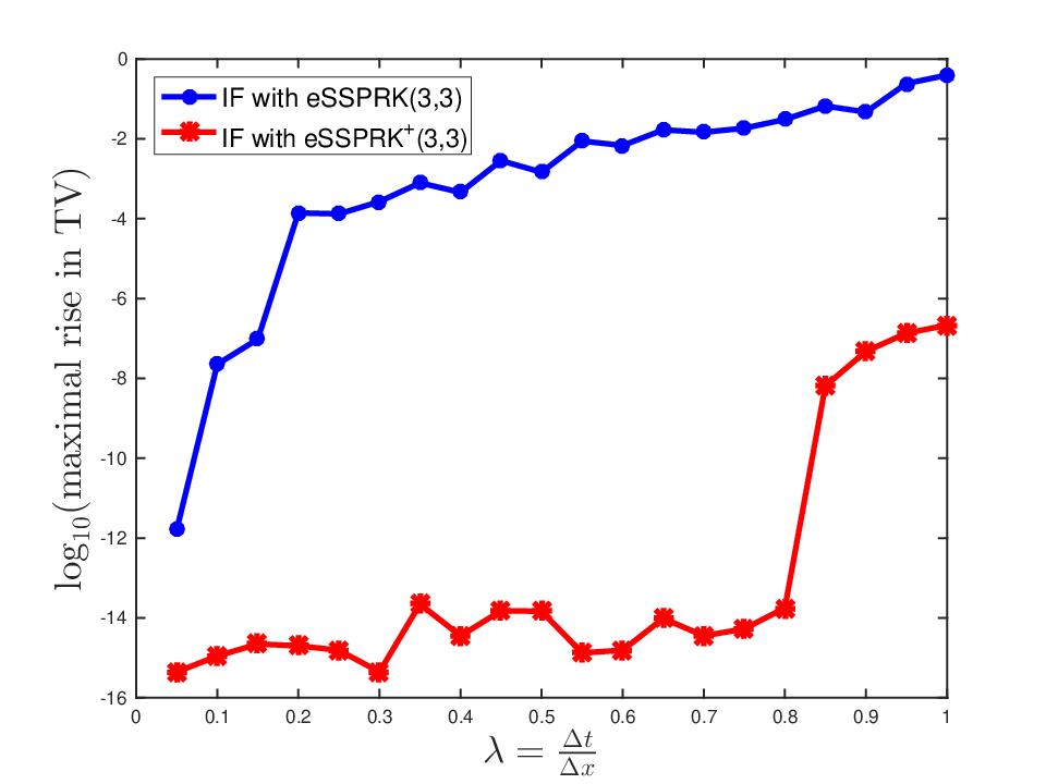
In Figure 1 we show the $\log_{10}$ of the maximal rise in total variation vs. the value of $\lambda=\frac{\Delta t}{\Delta x}$ of the evolution using (2.1) (in blue) and using (2.1) (in red). The results from (2.1) maintain a small maximal rise in total variation up to $\lambda\approx 0.8$, while in the results from (2.1) we observe that the maximal rise in total variation is large even for very small values of $\lambda$. This behavior is due to the fact that basing an integrating factor Runge–Kutta method on an explicit SSP Runge–Kutta method is not enough to ensure the preservation of a strong stability property – the method must also satisfy the non-decreasing abscissa condition to ensure that the strong stability property is preserved.

To understand the results in [15] recall that each stage of the explicit Runge–Kutta method (1.1) applied to the transformed problem (10) becomes

	$\displaystyle u^{(i)}$	$\displaystyle=$	$\displaystyle\sum_{j=0}^{i-1}\left(\alpha_{i,j}e^{L(t_{i}-t_{j})}u^{(j)}+\Delta t\beta_{i,j}e^{L(t_{i}-t_{j})}N(u^{(j)})\right)$
		$\displaystyle=$	$\displaystyle\sum_{j=0}^{i-1}\left(\alpha_{i,j}e^{L(c_{i}-c_{j})\Delta t}u^{(j)}+\Delta t\beta_{i,j}e^{L(c_{i}-c_{j})\Delta t}N(u^{(j)})\right)$
		$\displaystyle=$	$\displaystyle\sum_{j=0}^{i-1}e^{L(c_{i}-c_{j})\Delta t}\left(\alpha_{i,j}u^{(j)}+\Delta t\beta_{i,j}N(u^{(j)})\right).$

In the following, we consider each piece of this formula. Each of the following results is taken directly from [15] and the proofs appear in that work. We first consider the behavior of the exponential operator $e^{\tau L}$. The following theorem ensures that this term is strongly stable as long as $\tau\geq 0$:

Note that in the following results we no longer require the condition (9) but rather the weaker condition (14). Pairing this exponential with a forward Euler type step still preserves strong stability:

Finally, we put the pieces together:

In [15] we used these results to motivate the search for explicit SSP Runge–Kutta methods with non-decreasing abscissas, that would pair well with an integrating factor approach to produce SSPIFRK methods. We found explicit SSP Runge–Kutta methods of up to $s=10$ stages and order $p=4$ and demonstrated the performance of the corresponding explicit SSP integrating factor Runge–Kutta methods on widely used test cases.

In [16] we show that it is not absolutely necessary to have non-decreasing abscissas: even if there are some decreasing abscissas one can preserve the strong stability property by replacing the operator $L$ by an operator $\tilde{L}$ that satisfies

$$\|e^{-\tau\tilde{L}}u^{n}\|\leq\|u^{n}\|\;\;\;\;\forall\;\tau\geq 0,$$

whenever the difference of abscissas $c_{i}-c_{j}$ is negative. For hyperbolic partial differential equations, $\tilde{L}$ is simply the spatial discretization that is stable for the backwards in time version of the equation. This approach is employed in the classical SSP literature, called downwinding. In that case, negative coefficients $\beta_{i,j}$ preserve the SSP property as long as the operator is replaced by a downwinded operator [10, 11, 21].

In [22] a SSP optimization problem was defined for TSRK methods. The derivation of the optimization problem begins with the matrix form (19) of the TSRK:

$$\mathbf{w}=\mathbf{S}\mathbf{x}+\Delta t\mathbf{T}\mathbf{f}$$

We then add $r\mathbf{T}\mathbf{w}$ to each side of the method

$$\left(\mathbf{I}+r\mathbf{T}\right)\mathbf{w}=\mathbf{S}\mathbf{x}+r\mathbf{T}\left(\mathbf{w}+\frac{\Delta t}{r}\mathbf{f}\right)$$

and rearrange to obtain

$$\mathbf{w}=\mathbf{R}\mathbf{x}+\mathbf{P}\left(\mathbf{w}+\frac{\Delta t}{r}\mathbf{f}\right).$$

Where $\mathbf{P}=r\left(\mathbf{I}+r\mathbf{T}\right)^{-1}\mathbf{T}$ and $\mathbf{R}=\left(\mathbf{I}+r\mathbf{T}\right)^{-1}\mathbf{S}=\left(\mathbf{I}-\mathbf{P}\right)\mathbf{S}$. Note that the row sums of $[\mathbf{R}~\mathbf{P}]$ are each equal to one

$\displaystyle\mathbf{R}\mathbf{e}+\mathbf{P}\mathbf{e}=\left(\mathbf{I}-\mathbf{P}\right)\mathbf{S}\mathbf{e}+\mathbf{P}\mathbf{e}=\mathbf{I}\mathbf{S}\mathbf{e}-\mathbf{P}\mathbf{S}\mathbf{e}+\mathbf{P}\mathbf{e}=\mathbf{e}-\mathbf{P}\mathbf{e}+\mathbf{P}\mathbf{e}=\mathbf{e}.$

It is easy to see that if $\mathbf{R}$ and $\mathbf{P}$ have no negative values, then the method is a convex combination of forward Euler steps, and so is SSP with SSP coefficient defined by

$\displaystyle\mathcal{C}(\mathbf{S},\mathbf{T})$

$\displaystyle=\sup_{r}\left\{r:(\mathbf{I}+r\mathbf{T})^{-1}\mbox{ exists and }\mathbf{P}\geq 0,\mathbf{R}\geq 0\right\}.$

This leads directly to the optimization problem: We wish to find coefficients $\mathbf{T}$ and $\mathbf{S}$ for explicit SSP two-step Runge–Kutta methods that maximize the value of $r$ while satisfying

	$\displaystyle\left(\mathbf{I}+r\mathbf{T}\right)^{-1}\mathbf{S}\geq 0$		(22a)
	$\displaystyle r\left(\mathbf{I}+r\mathbf{T}\right)^{-1}\mathbf{T}\geq 0$		(22b)
	$\displaystyle\tau_{\rho}=0\;\;\;\mbox{for}\;\;\;\rho=1,...,p.$		(22c)

This requires that $\left(\mathbf{I}+r\mathbf{T}\right)^{-1}$ exists. The inequalities (22a) and (22b) are understood componentwise. The $\tau_{\rho}$ in (22c) are the order conditions listed in Appendix A.

In [22] a SSP optimization problem was defined for the TSRK methods, and optimized explicit TSRK methods of up to eighth order were found numerically. The SSP coefficients $\mathcal{C}$ of these methods up to seventh order are in Table 1. Of course, a method with more stages will have a higher SSP coefficient, but also require more computations. To account for this we define the effective SSP coefficient $\mathcal{C}_{\textup{eff}}=\frac{1}{s}\mathcal{C}$, which is the SSP coefficient normalized by the number of stages, in Table 2. An eleven stage eighth order method has an SSP cefficient $\mathcal{C}=0.341$ and an effective SSP Coefficient $\mathcal{C}_{\textup{eff}}=0.031$.

These methods break the fourth-order barrier of (one-step) SSP Runge–Kutta methods and have significantly larger SSP coefficients than the corresponding order multi-step methods. Numerical tests in [22] showed that these high order SSP two-step Runge-Kutta methods are beneficial for preserving the order and strong stability properties when used with high order spatial discretizations for the time integration of a variety of hyperbolic PDEs. It was proved in [22] that explicit SSP TSRK methods have order at most eight. In [23] it was shown that adding more steps overcomes this order barrier as well.

It can be easily shown that if we use an explicit SSP multi-step method

$\displaystyle u^{n+1}$

$\displaystyle=$

$\displaystyle\sum_{l=1}^{k}\left(\alpha_{l}u^{n-k+l}+\Delta t\beta_{l}F(u^{n-k+l})\right),$

(23)

which satisfies

$$u^{n+1}\leq\max_{l=1,...,k}\left\{\|u^{n-k+l}\|\right\}.$$

with SSP coefficient $\mathcal{C}=\max_{l}\frac{\alpha_{l}}{\beta_{l}}$, the result is SSP as well, with the same SSP coefficient:

Notice that for multi-step methods the notion of SSP includes all the previous steps considered.

However, SSP multi-step methods require many steps for high order and have small SSP coefficients as shown in [9]. Now that we see that building explicit SSP multi-step integrating factor methods is trivial, we are ready to approach the main question of this paper: is it possible to extend our results in [15] to two-step Runge–Kutta methods?

Any explicit SSP TSRK method of the form (18) that is SSP with SSP coefficient $\mathcal{C}=r$ can be re-written in the matrix-vector form (19), which can also be represented as

	$\displaystyle y_{1}$	$\displaystyle=u^{n}$
	$\displaystyle y_{i}$	$\displaystyle=v_{i,1}u^{n-1}+v_{i,2}u^{n}+\hat{\alpha}_{i}\left(u^{n-1}+\frac{\Delta t}{r}F(u^{n-1})\right)$		(26a)
		$\displaystyle+\sum_{j=1}^{i-1}\alpha_{i,j}\left(y_{j}+\frac{\Delta t}{r}F(y_{j})\right)\;\;\;\;2\leq i\leq s+1$
	$\displaystyle u^{n+1}$	$\displaystyle=y_{s+1},$

where $0\leq v_{i}\leq 1$, $\hat{\alpha}_{i}\geq 0$, and $\alpha_{i,j}\geq 0$. Here, the consistency condition $\mathbf{R}\mathbf{e}+\mathbf{P}\mathbf{e}=\mathbf{e}$ can be written as $v_{i,1}+v_{i,2}+\hat{\alpha}_{i}+\sum_{j=1}^{i-1}\alpha_{i,j}=1$ for each row $i$.

We note that the time-levels for each stage, also called the abscissas,

$$\mathbf{c}=\left(c_{1},c_{2},c_{3},...,c_{s},c_{s+1}\right)=\left(0,c_{2},c_{3},...,c_{s},1\right)$$

can be computed (in the matrix form) by $\mathbf{D}$, $\mathbf{A}$, and $\hat{\mathbf{A}}$ where $\mathbf{c}=\hat{\mathbf{A}}\mathbf{e}+\mathbf{A}\mathbf{e}-\mathbf{D}_{i,1}$. The abscissa corresponding to $u^{n}$ is $0$, the ones corresponding to all the internal stages $j=2,...,s$ are $c_{j}$ and the one corresponding to the final stage $u^{n+1}$ is $1$.

Applying (26) to the transformed equation becomes

	$\displaystyle y_{1}$	$\displaystyle=u^{n}$
	$\displaystyle y_{i}$	$\displaystyle=v_{i,1}e^{(c_{i}+1)\Delta t}u^{n-1}+v_{i,2}u^{n}+\hat{\alpha}_{i}e^{(c_{i}+1)\Delta t}\left(u^{n-1}+\frac{\Delta t}{r}N(u^{n-1})\right)$		(27a)
		$\displaystyle+\sum_{j=1}^{i-1}\alpha_{i,j}e^{(c_{i}-c_{j})\Delta t}\left(y_{j}+\frac{\Delta t}{r}N(y_{j})\right)\;\;\;\;2\leq i\leq s+1$
	$\displaystyle u^{n+1}$	$\displaystyle=y_{s+1}$

The following theorem tells us what conditions an explicit SSP TSRK method (26) has to satisfy to preserve the strong stability of a numerical solution when coupled with an integrating factor approach as in (27).

This theorem shows us that to find optimal SSP two-step Runge–Kutta methods that are suitable for use with the integrating factor approach, we must augment the optimization problem with additional conditions reflecting the need for non-decreasing abscissas.

To see how this theorem matters in practice, consider, once again, the motivating example in Subsection 2.1 where we solve Equation (11) using an integrating factor approach. In this case, we use $a=2$ so $Lu\approx-2u_{x}$. Otherwise, everything is the same as in Subsection 2.1. We evolve the transformed problem forward 25 time-steps for various time-steps using the eSSP-TSRK$(10,5)$ method in [22] and a new eSSP-TSRK${}^{+}(10,5)$ method that has non-decreasing abscissas. The $\log_{10}$ of the maximal rise in total variation at each stage vs. the value $\lambda=\frac{\Delta t}{\Delta x}$ is shown in Figure 2. We observe that the new method preserves the TVD behavior of the spatial discretization up to a large $\lambda$, while the eSSP-TSRK$(10,5)$ method in [22] does not preserve the TVD property of the spatial discretization.

Consider the van der Pol problem, a nonlinear system of ODEs of the form

	$\displaystyle u_{1}^{\prime}$	$\displaystyle=$	$\displaystyle u_{2}$
	$\displaystyle u_{2}^{\prime}$	$\displaystyle=$	$\displaystyle(-u_{1}+(1-u_{1}^{2})u_{2}).$

The problem can be written as $\mathbf{u}_{t}=L\mathbf{u}+N(\mathbf{u})$ where $\mathbf{u}=(u_{1};u_{2})$ and

$$L=\left(\begin{array}[]{rr}0&1\\ -1&0\\ \end{array}\right),\;\;\;N(\mathbf{u})=\left(\begin{array}[]{c}0\\ (1-u_{1}^{2})u_{2}\end{array}\right).$$

We initialize the problem with $\mathbf{u}_{0}=(2;0)$. Using a variety of SSPIF-TSRK methods, we run the problem to final time $T_{final}=2$, with $\Delta t=0.01,0.02,0.04,0.05,0.08,0.10$. The initial values and the exact solution (for error calculation) was calculated by Matlab’s ODE45 routine with tolerances set to AbsTol=$2\times 10^{-14}$ and RelTol=$2\times 10^{-14}$. We tested the SSPIF-TSRK methods based on the eSSP-TSRK⁺ methods whose SSP coefficients are presented in Table 3 above. We calculated the orders by finding the slopes of the $\log_{10}(errors)$ using Matlab’s polyfit function. The results, shown in Figure 4 for several selected methods, validate that the methods exhibit the expected order of convergence.

References

- [1] A.H. Al Mohy and N.J. Higham, Computing the action of the matrix exponential of a matrix, with an application to exponential integrators, SIAM Journal on Scientific Computing 33(2) (2011), pp. 488–511.
- [2] E. M. Constantinescu and A. Sandu, Optimal strong-stability-preserving general linear methods, SIAM Journal of Scientific Computing 32(5) (2010), pp. 3130-3150.
- [3] A.J. Christlieb, S. Gottlieb, Z. Grant, and D. C. Seal, Explicit Strong Stability Preserving Multistage Two-Derivative Time-Stepping Schemes, Journal of Scientific Computing 68(3) (2016), pp. 914-942.
- [4] S. Conde, S. Gottlieb, Z. Grant, J.N. Shadid, Implicit and Implicit-Explicit Strong Stability Preserving RungeÐKutta Methods with High Linear Order, Journal of Scientific Computing 73(2) (2017), pp. 667–690.
- [5] S. Cox and P. Matthews, Exponential time differencing for stiff systems, Journal of Computational Physics, 176 (2002), pp. 430–455.
- [6] L. Ferracina and M.N. Spijker, Strong stability of singly-diagonally-implicit Runge-Kutta methods, Applied Numerical Mathematics 58 (2008), pp. 1675-1686.
- [7] S. Gaudreault, G. Rainwater, M. Tokman, KIOPS: A fast adaptive Krylov subspace solver for exponential integrators, Journal of Computational Physics 372 (2018), pp. 236-255.
- [8] S. Gottlieb, Z. Grant, and L. Isherwood, Optimized strong stability preserving integrating factor two-step Runge–Kutta methods. https://github.com/SSPmethods/SSPIF-TSRK-methods.
- [9] S. Gottlieb, D. I. Ketcheson, and C.-W. Shu, Strong Stability Preserving Runge–Kutta and Multistep Time Discretizations, World Scientific Press, 2011.
- [10] S. Gottlieb and C.-W. Shu, Total variation diminishing Runge–Kutta methods, Mathematics of Computation, 67 (1998), pp. 73–85.
- [11] S. Gottlieb, C.-W. Shu, and E. Tadmor, Strong Stability Preserving High-Order Time Discretization Methods, SIAM Review, 43 (2001), pp. 89–112.
- [12] Z. Grant, S. Gottlieb, D.C. Seal, A Strong Stability Preserving Analysis for Explicit Multistage Two-Derivative Time-Stepping Schemes Based on Taylor Series Conditions, To appear in Communication on Applied Mathematics and Computation 1(1) (2019), pp. 21-59.
- [13] J.S. Hesthaven, Numerical methods for conservation laws: From analysis to algorithms, SIAM Publishing, Philadelphia (2017).
- [14] W. Hundsdorfer, S.J. Ruuth and R.J. Spiteri, Monotonicity-preserving linear multistep methods, SIAM Journal on Numerical Analysis 41 (2003), pp. 605–623.
- [15] L. Isherwood, S. Gottlieb, Z. Grant, Strong Stability Preserving Integrating Factor Runge–Kutta Methods. SIAM Journal on Numerical Analysis 56(6) (2018), pp. 3276–3307.
- [16] L. Isherwood, S. Gottlieb, Z. Grant, Downwinding for Preserving Strong Stability in Explicit Integrating Factor Runge–Kutta Methods, Pure and Applied Mathematics Quarterly 14(1) (2019), pp. 3-25.
- [17] G.-S. Jiang and C.-W. Shu, Efficient Implementation of Weighted ENO Schemes, Journal of Computational Physics 126(1) (1996), pp. 202-228.
- [18] D. I. Ketcheson, Highly efficient strong stability preserving Runge–Kutta methods with low-storage implementations, SIAM Journal on Scientific Computing, 30 (2008), pp. 2113–2136.
- [19] D.I. Ketcheson, C.B. Macdonald and S. Gottlieb, Optimal implicit strong stability preserving Runge-Kutta methods, Applied Numerical Mathematics 52 (2009), pp. 373–392.
- [20] D. I. Ketcheson, Computation of optimal monotonicity preserving general linear methods, Mathematics of Computation 78 (2009), pp. 1497–1513.
- [21] D. I. Ketcheson, Step sizes for strong stability preservation with downwind-biased operators, SIAM Journal on Numerical Analysis 49 (4) (2011), pp. 1649–1660.
- [22] D.I. Ketcheson, S. Gottlieb, and C. B. Macdonald, Strong stability preserving two- step Runge-Kutta methods, SIAM Journal on Numerical Analysis 49 (2012), pp. 2618-2639.
- [23] C. Bresten, S. Gottlieb, Z. Grant, D. Higgs, D.I. Ketcheson, and A. Nemeth, Explicit strong stability preserving multistep Runge-Kutta methods, Mathematics of Computation 86 (2017), pp. 747-769.
- [24] J. F. B. M. Kraaijevanger, Contractivity of Runge–Kutta methods, BIT, 31 (1991), pp. 482–528.
- [25] H.W.J. Lenferink, Contractivity-preserving implicit linear multistep methods, Mathematics of Computation 56 (1991), pp. 177–199.
- [26] R. J. LeVeque, Numerical Methods for Conservation Laws, ETH Lectures in Mathematics Series, Birkhauser-Verlag, (1990).
- [27] J. Niesen and W.M. Wright, Algorithm 919: A Krylov subspace algorithm for evaluating the -functions appearing in exponential integrators, ACM Transactions on Mathematical Software 38(3) (2012), pp. 22.
- [28] S. J. Ruuth and R. J. Spiteri, Two barriers on strong-stability-preserving time discretization methods, Journal of Scientific Computation, 17 (2002), pp. 211–220.
- [29] C.-W. Shu, Total-variation diminishing time discretizations, SIAM Journal on Scientific Statistical Computing 9 (1988), pp. 1073–1084.
- [30] C.-W. Shu and S. Osher, Efficient implementation of essentially non-oscillatory shock-capturing schemes, Journal of Computational Physics 77 (1988), pp. 439–471.
- [31] R.B. Sidje, EXPOKIT: A software package for computing matrix exponentials, ACM Transactions on Mathematical Software 24(1) (1998), pp. 130–156.
- [32] M.N. Spijker, Contractivity in the numerical solution of initial value problems, Numerische Mathematik 42 (1983), pp. 271–290.
- [33] M. Spijker, Stepsize conditions for general monotonicity in numerical initial value problems, SIAM Journal on Numerical Analysis, 45 (2008), pp. 1226–1245.
- [34] R. J. Spiteri and S. J. Ruuth, A new class of optimal high-order strong-stability-preserving time discretization methods, SIAM Journal on Numerical Analysis, 40 (2002), pp. 469–491.