Analytic view on Coupled Single-Electron Lines

The greatest simplification of matrix 8 is when we set all $t_{k^{\prime}\rightarrow m^{\prime}}=t_{o\rightarrow m}$ = $|t|$, and all $E_{p}(k)=E_{p}(m^{\prime})=E_{p}$ for $N$=3. Let us first consider the case of two insulating lines (all wells on each line are completely decoupled so there is no electron tunneling between the barriers and the barrier energies are high) where there are trapped electrons so $|t|=0$ (electrons are confined in quantum wells and cannot move towards neighbouring wells). In such a case, we deal with a diagonal matrix that has three different eigenvalues on its diagonal and has three different eigenenergy values

so $E_{3}<E_{2}<E_{1}$. In the limit of infinite distance between SELs, we have nine degenerate eigenergies. They are set to $E_{pk}$ which corresponds to six decoupled quantum systems (the first electron is delocalized into three upper wells, while the second electron is delocalized into three lowers wells).

Let us also consider the case of ideal metal where electrons are completely delocalized. In such a case, all $t_{k\rightarrow l(k^{\prime}\rightarrow l^{\prime})}$ $\gg$ $E_{p}(l(s^{\prime}))$ which brings Hamiltonian diagonal terms to be negligible in comparison with other terms. In such a case, we can set all diagonal terms to be zero which is an equivalent to the case of infinitely spaced SELs lines. It simply means that in the case of ideal metals, two lines are not ‘seeing’ each other.

Let us now turn to the case where processes associated with hopping between wells have similar values of energy to the energies denoted as $E_{p}(k(l^{\prime}))$. In such a case, the Hamiltonian matrix can be parametrized only by three real value numbers due to symmetries depicted in Fig. 1B (we divide the matrix by a constant number $|t|$) so

For a fixed $|t|$, we change the distance $d$ and observe that $q_{1_{1}}$ can be arbitrary large, while $q_{1_{2}}$ and $q_{1_{3}}$ have finite values for $d$=0. Going into the limit of infinite distance $d$, we observe that all $q_{1_{1}}$, $q_{1_{2}}$ and $q_{1_{3}}$ approach a finite value $\frac{2E_{p}}{|t|}$. We obtain the simplified Hamiltonian matrix that is a Hermitian conjugate and has a property $H_{k,k}=H_{N-k+1,N-k+1}$. It is in the form

We can analytically find nine energy eigenvalues and they correspond to the entangled states. We have

The last 3 energy eigenvalues are the most involving analytically and are the roots of a 3rd order polynomial

We omit writing direct and very lengthy formulas since the solutions of a 3rd-order polynomial are commonly known. The eigenvectors have the structure given in Appendix.

We can readily recognize that all nine energy eigenvectors are entangled. In particular, $\left|E_{1}\right\rangle=\left|1,0,0\right\rangle_{u}\left|1,0,0\right\rangle_{l}-\left|0,1,0\right\rangle_{u}\left|0,1,0\right\rangle_{l}+\left|0,0,1\right\rangle_{u}\left|0,0,1\right\rangle_{l}$ or $\left|E_{2}\right\rangle=\left|1,0,0\right\rangle_{u}\left|0,1,0\right\rangle_{l}-\left|0,1,0\right\rangle_{u}\left|1,0,0\right\rangle_{l}-\left|0,1,0\right\rangle_{u}\left|0,0,1\right\rangle_{l}+\left|0,0,1\right\rangle_{u}\left|0,1,0\right\rangle_{l}$, so they have no equivalence in the classical picture of two charged balls in channels that are repelling each other.

At first we are analyzing available spectrum of eigenenergies as in the case of insulator-to-metal phase transition [9], which can be implemented in a tight-binding model by a systematic increase of the hopping term from small to large values, while at the same time keeping all other parameters constant, as depicted in Fig.2. Described tight-binding model can minimic metal (t=1), semiconductor (t=0.1) and insulator state (t=0.01). We can recognized 2 SELs eigenergy spectra dependence on distance between two lines. Characteristic narrowing of bands is observed when one moves from big towards small distance d between SELs (what can be related to the ration of W/U in Hubbard model) and it is one of the signs of transition from metalic to insulator regime (Mott-insulator phase transition [9]). One of the plot referring to t=0.01 describes Anderson localization of electrons and in such case energy eigenspectra are determined by formula III-A and hopping terms $t$ can be completly neglected since electrons are localized in quantum well potential minimias.

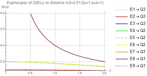
Bottom plots of Fig. 2. describe the ability of tunning eigenenergy spectra by change quantum well lenghts (a+b), $E_{p}$ and $t$ parameter. Last two parameters are directly voltage controlled as one is referring to Fig.1, where 8 voltage signals are used for controlling effective tight-binding Hamiltonian. It is informative to notice that change of quantum wells lenght expressed by a+b does not affect the eigenenergy of 2SELs significantly. Observed change changes the ratio of electrostatic to kinetic energy and thus is similar to the change in energy eigenspectra generated by different distances d. We can spot narrowing bands when we are moving from the situation of lower to the situation higher electrostatic energy of interacting electron and again it it typical for metal-insulator phase transition. Change of ratio kinetic to electrostatic energy can be obtained by keeping quantum well size constant, constant distance between 2 SELs and by change of hopping constant $t$ that is the measure of electron ability in conducting electric or heat current. Again one observes the narrowing of bands when we reduce t so the dominant energy of electron is due to electron-electron interaction. The last plot of Fig.2 describes our ability of tunning eigenenergy spectra of system in linear way just by change of $E_{p}$ parameter. In very real way we can recognize the ability of tunning the chemical potential (equivalent to Fermi energy at temperatures T=0K) by controlling voltages given in Fig.1. in our artifcial lattice system. Due to controllability of energy eigenspectra by controlling voltages from Fig.1 one can recognize 2 SELs system as the first stage of implementation of programmable quantum matter. In general case considered 2SELs Hamiltonian consists 6 different $E_{p}$ parameters and 6 different $t$ parameters that can be controlled electrostatically (12 parameters under electrostatic control) by 2SELS controlling voltages $V_{0}(t),..,V_{3}(t),V_{0^{\prime}}(t),..,V_{3^{\prime}}(t)$ depicted in Fig.1.

The numerical modeling of electron transport across coupled SELs is about solving a set of nine coupled recurrent equations of motion as it is in the case of time-dependent 2 SELs Hamiltonian. In this work we consider time-independent Hamiltonian implying constant occupation of energetic levels. Therefore the quantum state can be written in the form $\left|\psi(t^{\prime})\right\rangle$ $=\alpha_{1}e^{\frac{\hbar}{i}E_{1}t^{\prime}}\left|E_{1}\right\rangle+$..$+\alpha_{9}e^{\frac{\hbar}{i}E_{9}t^{\prime}}\left|E_{9}\right\rangle$, so the probability of occupancy of energetic level $E_{1}$ is $|\alpha_{1}|^{2}=|\left\langle E_{1}\right|\left|\psi(t)\right\rangle|^{2}=p_{E1}=constant$, etc. Since we have obtained analytical form of all states $\left|E_{k}\right\rangle$ and eigenenergies $E_{k}$ we have analytical form of quantum state dynamics $\left|\psi(t^{\prime})\right\rangle$ with time. From obtained analytical solutions presented in the Appendix we recognize that every eigenenergy state is the linear combination of positon-based states $\left|k\right\rangle\bigotimes\left|l^{\prime}\right\rangle$ what will imply that quantum state can never be fully localized at two nodes k and l’ as it is pointed by analytically obtained eigenstates of the 2SELs Hamiltonian that are given in the Appendix. In the conducted numerical simulations we visualize analytical solutions. We set $\hbar=1$ and $\alpha_{1}=..=\alpha_{8}=\frac{1}{9}$, $\alpha_{9}=\sqrt{1-\frac{8}{81}}$ or $\alpha_{1}=\alpha_{2}=\frac{1}{2}$,$\alpha_{9}=\frac{\sqrt{2}}{2}$,$\alpha_{3}=..=\alpha_{8}$ that will correspond to top or bottom plots of Fig.3. We can recognize that probability of occupancy of (1,1’) from Fig.1. (when two electrons are at input of 2SELs) is given by $|(\left\langle 1,0,0\right|\bigotimes\left\langle 1,0,0\right|)\left|\psi(t)\right\rangle|^{2}=|\gamma_{1}(t)|^{2}=p_{1}(t)$ (two electrons as SELs inputs) can be compared with occupancy of (3,3’) given by $p_{9}(t)=|\gamma_{9}(t)|^{2}=|(\left\langle 0,0,1\right|\bigotimes\left\langle 0,0,1\right|)\left|\psi(t)\right\rangle|^{2}$ (2 electrons at SELs outputs) as depicted in Fig. 3. We identify probability of finding first electron at input as the sum of $p_{1}(t)+p_{2}(t)+p_{3}(t)$.

Various symmetries can be traced in the bottom of Fig.3. as between probability $p_{2}(t)$ and $p_{8}(t)$ or in the upper part of Fig. 3 when $p_{2}(t)=p_{8}(t)$ or $\phi_{2}(t)=phase(\gamma_{2}(t))=\phi_{8}(t)$. The same symmetry relations applies to the case of probability $p_{4}(t)$ and $p_{6}(t)$ as well as $\phi_{4}(\gamma_{4}(t))$ and $\phi_{6}(\gamma_{6}(t))$. These symmetries has its origin in the fact that 2 SELs system is symmetric along x axes what can be recoginezed in symmetries of simplified Hamiltonian matrix 15. It shall be underlined that in the most general case when system matrix has no symmetries the energy eigenspectra might have less monotonic behaviour.

The quantum system dynamics over time is expressed by the equation of motion $\hat{H}(t^{\prime})\left|\psi(t^{\prime})\right\rangle=i\hbar\frac{d}{dt^{\prime}}\left|\psi(t^{\prime})\right\rangle$ that can be represented in discrete time step by relation $\frac{dt^{\prime}}{i\hbar}\hat{H}(t^{\prime})\left|\psi(t^{\prime})\right\rangle+\left|\psi(t^{\prime})\right\rangle=\left|\psi(t^{\prime}+dt^{\prime})\right\rangle$. It leads to the following equations of motion for quantum state expressed by equation (II) as follows

Symbol $[.]$ denotes functional dependence of $\vec{f}(\vec{\gamma}(t^{\prime}),dt^{\prime})$ on Hamiltonian $\hat{H}(t^{\prime})$. The measurement can be represented by projection operators $\hat{\Pi}(t^{\prime})$ equivalent to the matrix that acts on the quantum state over time. The lack of measurement can simply mean that the state projects on itself so the projection is the identity operation ($\hat{\Pi}(t^{\prime})=\hat{I}_{9\times 9}$). Otherwise, the quantum state is projected on its subset and hence the projection operator can change in a non-continuous way over time. We can formally write the quantum state dynamics with respect to time during the occurrence of measurement process (interaction of external physical system with the considered quantum system) as

Let us refer to some example by assuming that a particle in the upper SELs was detected by the upper output detector (Fig. 1b). In such a case, the following projector $\hat{\Pi}(t,t+\Delta t)$ is different from the identity in time interval $(t,t+\Delta t)$ with $1_{1_{t,t+\Delta t}}=1$ set to 1 in this time interval and 0 otherwise. The projector acts on the quantum state (diagonal matrix is given by diag symbol). It is given as

The repulsion (anticorrelation in position) of two electrons occurs in two parallel SELs and can be used in the construction of quantum SWAP gate. Therefore, the results obtained analytically and numerically on the two interacting SELs has its meaning in the development of quantum technologies [8] and also point to the interlink between the fundamental and applied science. It is important to underline that the tight-binding model allows for a quick detection of entangled states and for a transfer of this information into Schrödinger formalism, which has its importance in the design of quantum computer consisting of many coupled entangled qubits (fundamental modelling due to the large Hilbert space is limited to 10 qubits). Quite obviously, the Schrödinger equation gives detailed space resolution of quantum mechanical phenomena taking place in 2 or $N$ electrostatically coupled SELs that might contain an arbitrary number of quantum wells. Incorporation of spin effects is also possible in the given framework, but is beyond the scope of this work. The tight-binding model can be derived from the Schrödinger formalism (and vice versa) and is the simplistic version of the Hubbard model that is a very universal model capable of descring various collective phenomena in condensed matter physics. Therefore, it is expected that the tight-binding model can be also effective in describing physical effects in various programmable (electrostatically controlled) CMOS nanostructures. It shall be also underlined that the described position-dependent qubits are analogical to superconducting Cooper pair boxes where quantum phase transitions have been observed [4], [10]. The hopping term in the tight-binding model of semiconductor position-dependent qubits is analogical to energy of Josephson coupling in superconducting Cooper pair box (or in other types of superconducting qubits). Therefore, the existence of quantum phase transitions [11] is expected to occur in the studied SELs system since quantum phase transitions occurs in arrays of electrostatically coupled Josephson junctions. Therefore one is expecting to spot quantum phase transition in SELs coupled to superconducting Cooper pair boxes.

References

- [1] B.Patra, R.Incandela, J.Van Dijk, H.Homulle, L.Song, M.Shahmohammadi, R.B.Staszewski, and et al. Cryo-cmos circuits and systems for quantum computing applications. IEEE Journal of Solid-State Circuits, 53(1):309–321, 2018.
- [2] P. Giounanlis, E. Blokhina, K. Pomorski, D. R. Leipold, and R. B. Staszewski. Modeling of semiconductor electrostatic qubits realized through coupled quantum dots. IEEE Access, pages 1–16, 2019.
- [3] K.Pomorski, H.Akaike, A.Fujimaki, and K.Rusek. Relaxation method in description of ram memory cell in rsfq computer. COMPEL, 38(1):395–414, 2019
- [4] M.-S. Choi, J. Yi, M. Y. Choi, J. Choi, and S.-I. Lee. Quantum phase transitions in josephson-junction chains. Phys. Rev. B, 57:R716–R719, 1998.
- [5] H. Q. Xu. Method of calculations for electron transport in multiterminal quantum systems based on real-space lattice models. Phys. Rev. B, 66:165305,
- [6] T. Fujisawa, T. Hayashi, HD Cheong, YH Jeong, and Y. Hirayama. Rotation and phase-shift operations for a charge qubit in a double quantum dot. Physica E: Low-dimensional Systems and Nanostructures, 21(2-4):1046–1052, 2004.
- [7] K. D. Petersson, J. R. Petta, H. Lu, and A. C. Gossard. Quantum coherence in a one-electron semiconductor charge qubit. Phys. Rev. Lett., 105:246804, 2010.
- [8] P. Giounanlis, E. Blokhina, D. Leipold and R. B. Staszewski, ”Occupancy Oscillations and Electron Transfer in Multiple-Quantum-Dot Qubits and their Circuit Representation,” 2018 25th IEEE International Conference on Electronics, Circuits and Systems (ICECS), Bordeaux, 2018, pp. 153-156, doi: 10.1109/ICECS.2018.8618063
- [9] Jozef Spalek, Wstep do fizyki materii skondensowanej, PWN, 2015
- [10] D. Maile, S. Andergassen, and W. Belzig. Quantum phase transition with dissipative frustration. Phys. Rev. B, 97, 2018.
- [11] S.Sachdev. Quantum phase transitions. Cambridge Univ. Press, 2011.