Entrainment to Subharmonic Trajectories in
Oscillatory Discrete-Time SystemsThanks: An abridged version of this paper has been submitted to the 27th Mediterranean Conference on Control and Automation (MED 2019).

Rami Katz Michael Margaliot Emilia Fridman Thanks: This research was partially supported by research grants from the Israel Science Foundation and the Binational Science Foundation. Thanks: RK and EF are with School of Elec. Eng., Tel Aviv University, Israel. Thanks: MM (Corresponding Author) is with the School of Elec. Eng. and the Sagol School of Neuroscience, Tel-Aviv University, Tel-Aviv˜69978, Israel. E-mail: michaelm@eng.tau.ac.il

Abstract

A matrix $A$ is called totally positive (TP) if all its minors are positive, and totally nonnegative (TN) if all its minors are nonnegative. A square matrix $A$ is called oscillatory if it is TN and some power of $A$ is TP. A linear time-varying system is called an oscillatory discrete-time system (ODTS) if the matrix defining its evolution at each time $k$ is oscillatory. We analyze the properties of $n$ -dimensional time-varying nonlinear discrete-time systems whose variational system is an ODTS, and show that they have a well-ordered behavior. More precisely, if the nonlinear system is time-varying and $T$ -periodic then any trajectory either leaves any compact set or converges to an $(n-1)T$ -periodic trajectory, that is, a subharmonic trajectory. These results hold for any dimension $n$ . The analysis of such systems requires establishing that a line integral of the Jacobian of the nonlinear system is an oscillatory matrix. This is non-trivial, as the sum of two oscillatory matrices is not necessarily oscillatory, and this carries over to integrals. We derive several new sufficient conditions guaranteeing that the line integral of a matrix is oscillatory, and demonstrate how this yields interesting classes of discrete-time nonlinear systems that admit a well-ordered behavior.

Index Terms:

Nonlinear systems, totally positive matrices, totally nonnegative matrices, cooperative systems, entrainment, asymptotic stability, systems biology.

I Introduction

Positive dynamical systems arise naturally when the state-variables represent physical quantities that can only take nonnegative values [8, 20]. For example, in compartmental systems the state-variables represent the “density” at each compartment [24], in models of traffic flow or communication networks the state-variables represent the state of queues in the system [26], and in Markov chains the state-variables are probabilities [13].

Here, we introduce and analyze a new class of positive systems called oscillatory discrete-time systems. Recall that a matrix $A\in\mathbb{R}^{n\times m}$ is called totally positive (TP) if every minor of $A$ is positive, and totally nonnegative (TN) if every minor of $A$ is non-negative.¹¹ 1 Unfortunately, the terminology in this field is not uniform. We follow the terminology used in [7]. TN and TP matrices have a remarkable variety of interesting mathematical properties [7, 18]. One important property is that multiplying a vector by a TP matrix cannot increase the number of sign variations in the vector.

Oscillatory matrices are in the “middle ground” between TN and TP matrices. A matrix $A\in\mathbb{R}^{n\times n}$ is called oscillatory if $A$ is TN and there exists an integer $k>0$ such that $A^{k}$ is TP. For example, it is easy to verify that all the minors of

A:=\begin{bmatrix}0.2&0.1&0\\ 9&11&1\\ 0&1&3\end{bmatrix}

(1)

are nonnegative so $A$ is (TN) (but not TP as it has zero entries), and also that all the minors of $A^{2}=\begin{bmatrix}0.94&1.12&0.1\\ 100.8&122.9&14\\ 9&14&10\end{bmatrix}$ are positive, so $A$ is oscillatory.

The product of two TP/TN/oscillatory matrices is a TP/TN/oscillatory matrix, but the sum of two TP/TN/oscillatory matrices is not necessarily a TP/TN/oscillatory matrix. For example, the matrix $A=\begin{bmatrix}1&0.1\\ 9&1\end{bmatrix}$ and its transpose $A^{\prime}$ are TP (and thus in particular TN and oscillatory), yet $A+A^{\prime}=\begin{bmatrix}2&9.1\\ 9.1&2\end{bmatrix}$ is not TN (and thus not TP nor oscillatory), as $\det(A+A^{\prime})<0$ .

TP matrices have important applications in the asymptotic analysis of both continuous-time and discrete-time dynamical systems. Schwarz [25] introduced the notion of a totally positive differential system (TPDS). This is the linear time-varying (LTV) system

\dot{x}(t)=A(t)x(t),

(2)

satisfying that the associated transition matrix $\Phi(t_{1},t_{0})$ is TP for any pair $(t_{1},t_{0})$ with $t_{1}>t_{0}$ . The transition matrix is the matrix satisfying $x(t_{1})=\Phi(t_{1},t_{0})x(t_{0})$ for all $x(t_{0})\in\mathbb{R}^{n}$ . In the particular case where $A(t)\equiv A$ the transition matrix is $\Phi(t,t_{0})=\exp((t-t_{0})A)$ , and then (2) is TPDS iff $A$ is tridiagonal with positive entries on the super- and sub-diagonals. Schwarz used the VDP to show that the number of sign variations in $x(t)$ is a (integer-valued) Lyapunov function for the TPDS (2). It was recently shown [16] that TPDSs have important applications in the stability analysis of continuous-time nonlinear cooperative dynamical systems with a tridiagonal Jacobian.

An extension to discrete-time systems, called a totally positive discrete-time system (TPDTS), has been suggested recently [1]. The LTV

x(k+1)=A(k)x(k),

(3)

with $A:\mathbb{N}\to\mathbb{R}^{n\times n}$ , is called a TPDTS if $A(k)$ is TP for all $k\in\mathbb{N}$ . It was shown that time-varying nonlinear systems, whose variational equation is a TPDTS, satisfy strong asymptotic properties including entrainment to a periodic excitation. The variational equation is an LTV with a matrix described by a line integral of the Jacobian of the nonlinear system. Since the sum of two TP matrices is not necessarily TP, it is not trivial to verify that this line integral is indeed TP.

The main contributions of this paper are two-fold. First, we introduce the new notion of an oscillatory discrete-time system (ODTS). The LTV (3) is called an ODTS if $A(k)$ is oscillatory for all time $k$ . This is an important generalization of a TPDTS, as oscillatory matrices are much more common than TP matrices. We analyze the properties of discrete-time time-varying nonlinear systems, whose variational equation is an ODTS, and show that they satisfy useful asymptotic properties. In particular, if the $n$ -dimensional time-varying nonlinear system is $T$ -periodic then every solution either leaves every compact set or converges to an $(n-1)T$ -periodic solution, i.e. a subharmonic solution.

The variational equation associated with the nonlinear system is an LTV with a matrix described by a line integral of the Jacobian of the nonlinear system. Since the sum of two oscillatory matrices is not necessarily oscillatory, it is not trivial to verify that this line integral is indeed oscillatory.

The second contribution of this paper is deriving several new sufficient conditions guaranteeing that the line integral of a matrix is oscillatory. Our first condition considers the special case of a system with scalar nonlinearities. In this case we show that the integration can be performed in closed-form. The other conditions are based on sufficient conditions for a matrix to be oscillatory or TP. We demonstrate how these conditions yield new classes of discrete-time nonlinear systems with a well-ordered behavior.

The remainder of this paper is organized as follows: Section II reviews known definitions and results that will be used later on including the VDPs of TN and TP matrices, and TPDTSs. The next two sections describe our main results. Section III defines and analyzes ODTSs. Section IV provides several sufficient conditions verifying that the line integral of the Jacobian of a time-varying nonlinear system is oscillatory. This section also details several applications of the theoretical results. The final section concludes and describes several topics for further research.

We use standard notation. The set of nonnegative integers is $\mathbb{N}:=\{0,1,2,\dots\}$ . Matrices [vectors] are denoted by capital [small] letters. The transpose of a matrix $A$ is denoted $A^{\prime}$ . We use $\operatorname{diag}(v_{1},\dots,v_{n})$ to denote the $n\times n$ diagonal matrix with entries $v_{1},\dots,v_{n}$ on the diagonal.

II Preliminaries

We begin by reviewing the VDP of TN and TP matrices. More details and proofs can be found in the excellent monographs [7, 18, 9]. For a vector $z\in\mathbb{R}^{n}$ with no zero entries the number of sign variations in $z$ is

\sigma(z):=\left|\{i\in\{1,\dots,n-1\}:z_{i}z_{i+1}<0\}\right|.

(4)

For example, for $n=3$ consider the vector $z(\varepsilon):=\begin{bmatrix}2&\varepsilon&-3\end{bmatrix}^{\prime}$ . Then for any $\varepsilon\in\mathbb{R}\setminus\{0\}$ , $\sigma(z(\varepsilon))$ is well-defined and equal to one. More generally, the domain of definition of $\sigma$ can be extended, via continuity, to the set:

	$\displaystyle V:=$	$\displaystyle\{z\in\mathbb{R}^{n}:z_{1}\not=0,\;z_{n}\not=0,\;\text{and if }z_{i}=0$
		$\displaystyle\text{ for some~$i\in\{2,\dots,n-1\}$ then }z_{i-1}z_{i+1}<0\}.$

We recall two more definitions for the number of sign variations in a vector [7] that are well-defined for any $y\in\mathbb{R}^{n}$ . Let

s^{-}(y):=\sigma(\bar{y}),

where $\bar{y}$ is the vector obtained from $y$ by deleting all zero entries, and let

s^{+}(y):=\max_{x\in P(y)}\sigma(x),

where $P(y)$ is the set of all vectors obtained by replacing every zero entry of $y$ by either $-1$ or $+1$ . For example, for $y=\begin{bmatrix}-1&0&0&4\end{bmatrix}^{\prime}$ , $s^{-}(y)=1$ and $s^{+}(y)=3$ . These definitions imply that

0\leq s^{-}(y)\leq s^{+}(y)\leq n-1\text{ for all }y\in\mathbb{R}^{n}.

(5)

An important observation is that $s^{-}(y)=s^{+}(y)$ iff $y\in V$ .

A classical result [7] states that if $A\in\mathbb{R}^{n\times m}$ is TP then

s^{+}(Ax)\leq s^{-}(x)\text{ for all }x\in\mathbb{R}^{m}\setminus\{0\},

whereas if $A$ is TN (and in particular if it is TP) then

s^{-}(Ax)\leq s^{-}(x)\text{ for all }x\in\mathbb{R}^{m}.

(6)

These are the VDPs of TP and TN matrices. For example, the matrix $A=\begin{bmatrix}1&2\\ 1&4\end{bmatrix}$ is TP and for $x=\begin{bmatrix}1&-1\end{bmatrix}^{\prime}$ , we have

s^{+}(Ax)=s^{+}(\begin{bmatrix}-1&-3\end{bmatrix}^{\prime})<s^{-}(x).

For square matrices (which is the relevant case when considering the transition matrices of dynamical systems) more precise results are known. Recall that a matrix is called strictly sign-regular of order $k$ (denoted $SSR_{k}$ ) if its minors of order $k$ are either all positive or all negative. For example, $A=\begin{bmatrix}1&2\\ 3&4\end{bmatrix}$ is $SSR_{1}$ because all its entries are positive, and $SSR_{2}$ because it single minor of order $2$ is negative. It was recently shown [3] that if $A\in\mathbb{R}^{n\times n}$ is non-singular then for any $k\in\{1,\dots,n-1\}$ we have that $A$ is $SSR_{k}$ iff

x\in\mathbb{R}^{n}\setminus\{0\}\text{ and }s^{-}(x)\leq k-1\implies s^{+}(Ax)\leq k-1.

For example, for $k=1$ this implies that for a non-singular matrix $A\in\mathbb{R}^{n\times n}$ the following two conditions are equivalent: (1) all the entries of $A$ are either all positive or all negative; and (2) for every $x\not=0$ with all entries non-negative or all non-positive the vector $Ax$ has all entries positive or all negative.

We now review applications of total positivity to discrete-time dynamical systems.

II-A Totally Positive Discrete-Time Systems

Consider the discrete-time LTV (3) with $A:\mathbb{N}\to\mathbb{R}^{n\times n}$ . The system is called a TPDTS [1] if $A(k)$ is TP for all $k\in\mathbb{N}$ . Intuitively speaking, this is the discrete-time analogue of a TPDS. The VDP and (5) imply that for any $x(0)\in\mathbb{R}^{n}\setminus\{0\}$ we have

\dots\leq s^{-}(x(1))\leq s^{+}(x(1))\leq s^{-}(x(0))\leq s^{+}(x(0)).

(7)

In other words, both $s^{-}(x(k))$ and $s^{+}(x(k))$ can be viewed as integer-valued Lyapunov functions for the trajectories of a TPDTS. Furthermore, there can be no more then $n-1$ strict inequalities in (7), as $s^{-}$ and $s^{+}$ take values in $\{0,1,\dots,n-1\}$ . This implies that there exists $m\in\mathbb{N}$ such that $s^{-}(x(k))=s^{+}(x(k))$ for all $k\geq m$ , i.e. $x(k)\in V$ for all $k\geq m$ . In particular, $x_{1}(k)\not=0$ (and $x_{n}(k)\not=0$ ) for all $k\geq m$ . Moreover, it was shown in [1] that there exists $p\in\mathbb{N}$ such that the following eventual monotonicity property holds: either $x_{1}(k)>0$ for all $k\geq p$ or $x_{1}(k)<0$ for all $k\geq p$ (and similarly for $x_{n}(k)$ ).

This property can be applied to study the asymptotic properties of time-varying nonlinear discrete-time systems. Consider the system

x(k+1)=f(k,x(k)).

(8)

We assume that $f:\mathbb{N}\times\mathbb{R}^{n}\to\mathbb{R}^{n}$ is $C^{1}$ with respect to its second variable, and denote its Jacobian by $J(k,x):=\frac{\partial}{\partial x}f(k,x)$ . We also assume that the trajectories of (8) evolve on a compact and convex state-space $\Omega\subset\mathbb{R}^{n}$ . For $a\in\Omega$ and $j\in\mathbb{N}$ , let $x(j,a)$ denote the solution of (8) at time $j$ with $x(0)=a$ .

Fix $a,b\in\Omega$ and let $z(k):=x(k,b)-x(k,a)$ . Then (see, e.g. [1])

z(k+1)=M(k)z(k),

(9)

where

\displaystyle M(k)=M(k,a,b):=\int_{0}^{1}J(k,rx(k,b)+(1-r)x(k,a))\mathop{}\!\mathrm{d}r.

(10)

The LTV system (9) is called the variational equation associated with (8), as it describes how the variation between the two solutions $x(k,b)$ and $x(k,a)$ evolves in time.

We pose two assumptions.

Assumption 1

The matrix

F(k,a,b):=\int_{0}^{1}J(k,ra+(1-r)b)\mathop{}\!\mathrm{d}r

(11)

is TP for all $k\in\mathbb{N}$ and all $a,b\in\Omega$ .

Note that this implies that (9) is a TPDTS.

Assumption 2

There exists $T\in\{1,2,\dots\}$ such that the map in (8) is $T$ -periodic, that is,

f(k,a)=f(k+T,a)\text{ for all }k\in\mathbb{N}\text{ and all }a\in\Omega.

Note that in the particular case where $f$ is time-invariant this holds (vacuously) for every $T\in\mathbb{N}$ .

Theorem 1

[1] If Assumptions 1 and 2 hold then every solution of (8) emanating from $\Omega$ converges to a $T$ -periodic solution of (8).

If the time-dependence in $f$ is due to an input (or excitation) $u$ , that is, $f(k,x(k))=g(u(k),x(k))$ for some map $g$ then Assumption 2 holds if $u$ is $T$ -periodic. Thm. 1 then implies that the system entrains to the periodic excitation, as every solution converges to a periodic solution with the same period $T$ . Entrainment is an important property in many natural and artificial systems [14, 15, 23]. For example, many biological processes in our bodies, like the sleep-wake cycle, entrain to the 24h-periodic solar day.

In the special case where $f$ is time-invariant Thm. 1 yields the following result.

Corollary 1

[1] Consider the time-invariant nonlinear system

x(k+1)=f(x(k))

(12)

whose trajectories evolve on a compact and convex state-space $\Omega\subset\mathbb{R}^{n}$ . Suppose that

F(a,b):=\int_{0}^{1}J(ra+(1-r)b)\mathop{}\!\mathrm{d}r

(13)

is TP for all $a,b\in\Omega$ . Then every solution of (12) emanating from $\Omega$ converges to an equilibrium point.

Note that the equilibrium point is not necessarily unique.

The condition on $F(a,b)$ implies that every minor of $J(x)$ is positive for all $x\in\Omega$ . In particular, the first-order minors, i.e. the entries of $J(x)$ are positive, so the nonlinear system is strongly cooperative [31, 29]. The conditions here require more than strong cooperativity and as a consequence yield more powerful results on the asymptotic behavior of the system (see, e.g. [30, 11]).

In the particular case of planar systems, the conditions here require that the entries of $J(x)$ are positive, and that $\det J(x)$ is positive. The latter condition is known to be an orientation-preserving condition that has been used in the analysis of planar cooperative systems [30].

The next result, which seems to be new, shows that total positivity (in fact, a slightly weaker condition) implies an orientation-preserving property (with respect to a specific order) for any dimension $n$ . For two vectors $x,y\in\mathbb{R}^{n}$ , we write $x\ll y$ if $x_{i}<y_{i}$ for all $i\in\{1,\dots,n\}$ . Let $D_{\pm}\in\mathbb{R}^{n\times n}$ be the diagonal matrix with $d_{ii}=(-1)^{i+1}$ for all $i\in\{1,\dots,n\}$ . Note that $(D_{\pm})^{-1}=D_{\pm}$ . We say that $z\in\mathbb{R}^{n}$ is alternating if $z_{i}z_{i+1}<0$ for all $i\in\{1,\dots,n-1\}$ . This implies of course that $s^{-}(z)=s^{+}(z)=n-1$ .

Lemma 1

Let $P\in\mathbb{R}^{n\times n}$ be TN and nonsingular. If $x,y\in\mathbb{R}^{n}$ are such that

D_{\pm}PD_{\pm}x\ll D_{\pm}PD_{\pm}y

(14)

then

x\ll y.

The proof is placed in the Appendix.

Example 1

Consider the TP matrix $P=\begin{bmatrix}1&2\\ 3&8\end{bmatrix}$ . Then (14) becomes $\begin{bmatrix}1&-2\\ -3&8\end{bmatrix}(x-y)\ll 0$ and this holds iff $x_{1}-y_{1}<0$ and $\frac{3}{8}<\frac{x_{2}-y_{2}}{x_{1}-y_{1}}<\frac{1}{2}$ , so in particular $x\ll y$ .

In the context of the LTV $z(k+1)=Pz(k)$ , $z(0)=z_{0}\in\mathbb{R}^{n}$ , Lemma 1 implies the following. Suppose that $P$ is TN and non-singular and let $y(k):=D_{\pm}z(k)$ . Then it is not possible that for some $i\geq 1$ we have

y(0)\ll y(1)\ll\dots\ll y(i-1)\ll y(i)\text{ and }y(i)\gg y(i+1).

(15)

Indeed, the last inequity here yields

D_{\pm}PD_{\pm}y(i-1)\gg D_{\pm}PD_{\pm}y(i),

so Lemma 1 gives

y(i-1)\gg y(i),

and this contradicts (15).

Smillie [27] and Smith [28] proved convergence to an equilibrium and entrainment in a certain class of continuous-time nonlinear dynamical systems. Their results are based on using the number of sign variations in the solution of the associated (continuous-time) variational system as an integer-valued Lyapunov function. It was recently shown that these results are closely related to the theory of TPDSs [16]. Thm. 1 and Corollary 1 may be regraded as discrete-time analogues of these results.

It is well-known that asymptotically stable linear systems entrain to periodic excitations. However, nonlinear systems do not necessarily entrain. This is true even for strongly monotone systems. Ref. [32] provides interesting examples of continuous-time, strongly cooperative dynamical systems whose vector field is $T$ periodic and admit a solution that is periodic with minimal period $nT$ , for any integer $n\geq 2$ . Furthermore, this subharmonic solution may be asymptotically stable.

In order to apply Thm. 1 and Corollary 1 one needs to verify that the line integral of the Jacobian is TP. This is not trivial because the sum of two TP matrices is not necessarily a TP matrix, and this is naturally carried over to integrals.

Example 2

It is straightforward to verify that $A(t)=\begin{bmatrix}1.01&t+1\\ \frac{1}{t+1}&1\end{bmatrix}$ is TP for all $t\in[0,1]$ , yet $\int_{0}^{1}A(t)\mathop{}\!\mathrm{d}t=\begin{bmatrix}1.01&3/2\\ \ln(2)&1\end{bmatrix}$ is not TP (and not even TN), as it has a negative determinant.

A matrix $A\in\mathbb{R}^{n\times n}$ is called oscillatory if it is TN and there exists $k\in\mathbb{N}$ such that $A^{k}$ is TP. The smallest such $k$ is called the exponent of the oscillatory matrix $A$ . Oscillatory matrices are in the “middle ground” between TN and TP matrices, and are much more common than TP matrices in applications. Indeed, it is well-known that a TN matrix $A\in\mathbb{R}^{n\times n}$ is oscillatory if and only if it is non-singular and irreducible [7, Ch. 2], and that in this case $A^{n-1}$ is TP. The next example demonstrates this.

Example 3

Consider the tridiagonal matrix

A=\begin{bmatrix}a_{1}&b_{1}&0&\dots&0\\ c_{1}&a_{2}&\ddots&\dots&\vdots\\ 0&\ddots&\ddots&\dots&\vdots\\ \vdots&\ddots&\ddots&\dots&b_{n-1}\\ 0&\dots&\dots&c_{n-1}&a_{n}\end{bmatrix}

(16)

with $b_{i},c_{i}\geq 0$ for all $i$ . In this case, the dominance condition

a_{i}\geq b_{i}+c_{i-1}\quad\text{for all }i\in\{1,\dots,n\},

(17)

with $c_{0}:=0$ and $b_{n}:=0$ , guarantees that $A$ is TN (see e.g. [7, Ch. 0]). If, furthermore, $b_{i},c_{i}>0$ for all $i$ then $A$ is irreducible. Thus, if $A$ is also non-singular then it is oscillatory.

The next two sections describe our main results.

III Oscillatory Discrete-Time Systems

We begin by introducing the new notion of an ODTS.

Definition 1

The discrete-time LTV

y(k+1)=A(k)y(k),

(18)

with $A:\mathbb{N}\to\mathbb{R}^{n\times n}$ , is called an ODTS of order $p$ if $A(k)$ is oscillatory for all $k\in\mathbb{N}$ , and every product of $p$ matrices in the form:

A(k_{p})\dots A(k_{2})A(k_{1}),\quad 0\leq k_{1}<\dots<k_{p},

is TP.

For example, if $A(k)$ is TP for all $k$ then (18) is an ODTS of order $1$ . Also, since the product of any $n-1$ oscillatory matrices is TP [18], (18) is always an ODTS of order $n-1$ .

We now describe the applications of ODTS to the time-varying nonlinear system:

x(k+1)=f(k,x(k)),

(19)

where $f(k,x)$ satisfies Assumption 2. We assume that the trajectories of (19) evolve in a compact and convex state-space $\Omega\in\mathbb{R}^{n}$ . For $k\in\mathbb{N}$ and $a,b\in\Omega$ , let

F(k,a,b):=\int_{0}^{1}J(k,ra+(1-r)b)\mathop{}\!\mathrm{d}r.

We pose the following assumption.

Assumption 3

The system

z(k+1)=F(k,\cdot,\cdot)z(k)

(20)

is an ODTS of order $h$ .

We can now state the main result in this section.

Theorem 2

Suppose that Assumptions 2 and 3 hold. Let $u:=hT$ . Then every solution of (19) emanating from $\Omega$ converges to a $u$ -periodic solution of (19).

Remark 1

If $F(k,a,b)$ is TP for all $k\in\mathbb{N}$ and all $a,b\in\Omega$ then Assumption 3 holds with $h=1$ so Thm. 2 implies that every solution of (19) emanating from $\Omega$ converges to a $T$ -periodic solution of (19). This recovers the TPDS case. If $F(k,a,b)$ is oscillatory for all $k\in\mathbb{N}$ and all $a,b\in\Omega$ then in particular every product of $n-1$ matrices is TP, so Thm. 2 implies that every solution of (19) emanating from $\Omega$ converges to an $(n-1)T$ -periodic solution of (19).

Remark 2

The LTV (18) is of course a special case of (19) with Jacobian $J(k,x(k))=A(k)$ , and thus $F(k,a,b)=A(k)$ for all $a,b\in\Omega$ and all $k\in\mathbb{N}$ . We conclude that if $A(k)=A(k+T)$ for all $k\in\mathbb{N}$ then every solution of an ODTS of order $h$ converges to periodic solution of (18) with period $u:=hT$ .

Proof:

Pick $\alpha,\beta\in\Omega$ with $\alpha\neq\beta$ . Let

z(k):=x(k,\beta)-x(k,\alpha)

and recall that $z$ satisfies the variational equation (9), with

M(k,\alpha,\beta):=\int_{0}^{1}J(k,rx(k,\beta)+(1-r)x(k,\alpha))\mathop{}\!\mathrm{d}r.

Assumption 3 implies that $M(k,\alpha,\beta)$ is oscillatory. Let $v(k):=z(ku)$ . Then

v(k+1)=M((k+1)u-1,\alpha,\beta)\dots M(ku,\alpha,\beta)v(k).

(21)

The product on the right-hand side includes $u=hT$ matrices, and is TP, as the product of any $h$ matrices is TP, and the product of any two TP matrices is TP. Thus, (21) is a TPDS. Thm. 6 in [1] implies the following eventual monotonicity property: there exists $m\in\mathbb{N}$ such that either $v_{1}(k)>0$ for all $k\geq m$ or $v_{1}(k)<0$ for all $k\geq m$ .

Pick $a\in\Omega$ and let $x(k,a)$ denote the trajectory of (19) emanating from $a$ . Let $b:=x(u,a)$ . If $x(k,a)$ is $u$ -periodic then there is nothing to prove. Therefore, we can assume that the trajectories $x(k,a)$ and $x(k,b)$ are not identical. Note that Assumption 2 implies that both trajectories are solutions of (19). By the eventual monotonicity property, there exists $m\in\mathbb{N}$ such that, without loss of generality,

\displaystyle x_{1}((k+1)u,a)-x_{1}(ku,a)>0\text{ for all }k\geq m.

(22)

Let

	$\displaystyle\omega_{u}(a):=\{$	$\displaystyle p:\text{ there exist }m_{i}\in\mathbb{N}\text{ with }m_{1}<m_{2}<\dots$
		$\displaystyle\text{ such that }\lim_{i\to\infty}x(m_{i}u,a)=p\},$

that is, the $u$ -omega limit set corresponding to $a$ . By compactness of $\Omega$ it follows that $\omega_{u}(a)\neq\emptyset$ . We now show that $\omega_{u}(a)$ is a singleton. Assume that there exist $p,q\in\omega_{u}(a)$ , with $p\neq q$ . We claim that $p_{1}=q_{1}$ . Indeed, there exist sequences $\left\{m_{k}\right\}_{k=1}^{\infty}$ and $\left\{s_{k}\right\}_{k=1}^{\infty}$ such that $p=\lim_{m_{k}\to\infty}x(m_{k}u,a)$ and $q=\lim_{s_{k}\to\infty}x(s_{k}u,a)$ . Passing to sub-sequences, if needed, we may assume that $m_{k}<s_{k}<m_{k+1}$ for all $k\in\mathbb{N}$ . Now (22) implies that $p_{1}=q_{1}$ . We conclude that any two points in $\omega_{u}(a)$ have the same first coordinate.

Consider the trajectories emanating from $p$ and $q$ , that is, $x(k,p)$ and $x(k,q)$ . Since $p,q\in\omega_{u}(a)$ and $\omega_{u}(a)$ is an invariant set,

x(ku,p),x(ku,q)\in\omega_{u}(a)\text{ for all }k\in\mathbb{N}.

This implies that

x_{1}(ku,p)=x_{1}(ku,q)\text{ for all }k\in\mathbb{N}.

However, this contradicts the eventual monotonicity of (21). We conclude that $\omega_{u}(a)$ is a singleton, and this completes the proof. ∎

Remark 3

Note that the proof of Thm. 2 relies on the fact that any product of $u=hT$ matrices in (21) is TP. In practice, it may be the case that a product of a smaller number of matrices in the variational equation is TP. In this case, every solution $x(k,a)$ will converge to a periodic solution of (19) with period less than $hT$ . Nevertheless, the minimal period of the limit solution must divide $hT$ .

The next subsection provides several sufficient conditions guaranteeing that Assumption 3 indeed holds, and applications to several dynamical systems.

IV Conditions guaranteeing that a matrix line integral is oscillatory

Our first sufficient condition is based on the sufficient condition for a matrix to be oscillatory described in Example 3.

IV-A Discretizing nonlinear tridiagonal strongly cooperative systems

Consider the nonlinear time-varying dynamical system $\dot{x}=f(t,x)$ . Let

x(k+1)=x(k)+\varepsilon f(k,x(k))

(23)

denote its Euler discretization, with $\varepsilon>0$ .

Lemma 2

Suppose that the trajectories of (23) evolve on a compact and convex set $\Omega\subset\mathbb{R}^{n}$ , and that

J(k,a):=I+\varepsilon\frac{\partial}{\partial x}f(k,a)

(24)

is tridiagonal, with positive entries on the super- and sub-diagonals for all $k\in\mathbb{N}$ and all $a\in\Omega$ . Then for any $\varepsilon>0$ sufficiently small Assumption 3 holds with $h=n-1$ .

Note that since $J(k,a)$ is tridiagonal, it is not TP, so the TPDTS framework cannot be used to analyze this case.

Proof:

Pick $k\in\mathbb{N}$ and $a\in\Omega$ . The assumptions on the Jacobian imply that $J(k,a)$ is irreducible for all $\varepsilon>0$ , and nonsingular for every $\varepsilon>0$ sufficiently small. Also, $J(k,a)$ satisfies the dominance condition described in Example 3 for any $\varepsilon>0$ sufficiently small, and is thus TN. Furthermore, all these properties carry over to the matrix $F$ defined in (20). ∎

The next example demonstrates Lemma 2 in a simple case.

Example 4

Consider the continuous-time system:

\dot{x}=\begin{bmatrix}0&1&0\\ 1&0&1\\ 0&1&0\end{bmatrix}x.

Its Euler discretization is $x(k+1)=Ax(k)$ with

A:=\begin{bmatrix}1&\varepsilon&0\\ \varepsilon&1&\varepsilon\\ 0&\varepsilon&1\end{bmatrix},

with $\varepsilon>0$ . The matrix $A$ is irreducible, and it is nonsingular for any $\varepsilon\not=1/\sqrt{2}$ . Combining this with Example 3 implies that $A$ is oscillatory for any $\varepsilon\in(0,1/2]$ . The eigenvalues of $A$ are

	$\displaystyle\lambda_{1}$	$\displaystyle:=1+\varepsilon\sqrt{2},$
	$\displaystyle\lambda_{2}$	$\displaystyle:=1,$
	$\displaystyle\lambda_{3}$	$\displaystyle:=1-\varepsilon\sqrt{2},$

with corresponding eigenvectors

	$\displaystyle v^{1}$	$\displaystyle:=\begin{bmatrix}1,\sqrt{2},1\end{bmatrix}^{\prime},$
	$\displaystyle v^{2}$	$\displaystyle:=\begin{bmatrix}-1,0,1\end{bmatrix}^{\prime},$
	$\displaystyle v^{3}$	$\displaystyle:=\begin{bmatrix}1,-\sqrt{2},1\end{bmatrix}^{\prime}.$

Pick $x(0)\in\mathbb{R}^{3}$ . Let $c_{i}\in\mathbb{R}$ be such that $x(0)=\sum_{i=1}^{3}c_{i}v^{i}.$ Then

x(k)=\sum_{i=1}^{3}c_{i}\lambda_{i}^{k}v^{i},

and this implies that for any $\varepsilon\in(0,1/2]$ any solution $x(k)$ that remains in a compact set converges to either $c_{1}v^{1}$ or to the origin.

The next example describes an application of Lemma 2 to a nonlinear model from systems biology.

Example 5

Cells often sense and respond to various stimuli by modification of protein production. One mechanism for this is phosphorelay (also called phosphotransfer), in which a phosphate group is transferred through a serial 1D chain of proteins from an initial histidine kinase (HK) down to a final response regulator (RR). The nonlinear compartmental system:

$\displaystyle\dot{x}_{1}$	$\displaystyle=(p_{1}-x_{1})c-\eta_{1}x_{1}(p_{2}-x_{2})-\xi_{1}x_{1},$
$\displaystyle\dot{x}_{2}$	$\displaystyle=\eta_{1}x_{1}(p_{2}-x_{2})-\eta_{2}x_{2}(p_{3}-x_{3})-\xi_{2}x_{2},$

$\displaystyle\dot{x}_{n-1}$	$\displaystyle=\eta_{n-2}x_{n-2}(p_{n-1}-x_{n-1})-\eta_{n-1}x_{n-1}(p_{n}-x_{n})$
	$\displaystyle-\xi_{n-1}x_{n-1},$
$\displaystyle\dot{x}_{n}$	$\displaystyle=\eta_{n-1}x_{n-1}(p_{n}-x_{n})-\eta_{n}x_{n},$	(25)

has been suggested as a model for phosphorelay [6]. Here $c:[t_{1},\infty)\to\mathbb{R}_{+}$ is the strength at time $t$ of the stimulus activating the HK, $x_{i}(t)$ is the concentration of the phosphorylated form of the protein at the $i$ ’th layer at time $t$ , the parameter $p_{i}>0$ denotes the total protein concentration at that layer, and $\eta_{i},\xi_{i}>0$ are parameters that describe reaction rates. Note that $\eta_{n}x_{n}(t)$ is the flow at time $t$ of the phosphate group to an external receptor molecule.

In the particular case where $p_{i}=1$ and $\xi_{i}=0$ for all $i$ Eq. (5) becomes the ribosome flow model (RFM) [22]. This is the dynamic mean-field approximation of a fundamental model from non-equilibrium statistical physics called the totally asymmetric simple exclusion process (TASEP) [4]. The RFM describes the unidirectional flow along a chain of $n$ sites. The state-variable $x_{i}\in[0,1]$ describes the normalized occupancy at site $i$ , where $x_{i}=0$ [ $x_{i}=1$ ] means that site $i$ is completely free [full], and $\eta_{i}$ is the capacity of the link that connects site $i$ to site $i+1$ . This has been used to model and analyze mRNA translation (see, e.g., [19, 21, 17, 34]), where every site corresponds to a group of codons on the mRNA strand, $x_{i}(t)$ is the normalized occupancy of ribosomes at site $i$ at time $t$ , $c(t)$ is the initiation rate at time $t$ , and $\eta_{i}$ is the elongation rate from site $i$ to site $i+1$ .

Write (5) as $\dot{x}=f(x)$ . Then $\frac{\partial}{\partial x}f(x)$ is tridiagonal, with entries $\eta_{i}x_{i}$ on the super-diagonal, and $\eta_{i}(p_{i+1}-x_{i+1})$ , $i=1,\dots,n-1$ , on the sub-diagonal.

Consider the corresponding discretized system (23). It is not difficult to show that $\Omega:=[0,p_{1}]\times\dots\times[0,p_{n}]$ is an invariant set of (23) for any $\varepsilon>0$ sufficiently small. Furthermore, for any $a\in\Omega$ we have that $x(k,a)\in\operatorname{int}(\Omega)$ for all $k\geq 1$ and then the conditions in Lemma 2 on $J(k,a)$ defined in (24) hold. Fig. 1 depicts the trajectories of the discretized system with $n=4$ , $\varepsilon=0.1$ , $\xi_{i}=3$ , $\eta_{i}=1$ , $p_{1}=0.8$ , $p_{2}=p_{3}=p_{4}=2$ , initial condition $x(0)=\begin{bmatrix}0.5&0.1&0.6&0.3\end{bmatrix}^{\prime}$ , and the periodic stimulus $c(k)=3+\sin(k\pi/4)$ . Note that this means that the map is $T$ -periodic with (minimal) period $T=8$ . Combining Thm. 2 and Lemma 2, we conclude that any solution of the discretized system converges to a periodic solution with period $(n-1)T=24$ . It may be seen that the specific solution depicted in Fig. 1 converges to a periodic solution with period $8$ .

Refer to caption — Fig. 1: The trajectory $x_{1}(k)$ (marked by o), $x_{2}(k)$ (*), $x_{3}(k)$ (x), and $x_{4}$ (+) in Example 5.

In general, our approach is to find sufficient conditions guaranteeing that the line integral of a matrix is oscillatory without actually calculating the integral. However, there is an important special case where the integral can be computed explicitly.

IV-B The case of strictly monotone scalar nonlinearities

Let $f_{i}:\mathbb{R}\to\mathbb{R}$ , $i=1,\dots,n$ , be $C^{1}$ functions such that

f^{\prime}_{i}(y):=\frac{d}{dy}f_{i}(y)>0\text{ for all }i\text{ and all }y\in\mathbb{R}.

(26)

Consider the time-varying nonlinear system:

x(k+1)=C(k)\begin{bmatrix}f_{1}(x_{1}(k))\\ f_{2}(x_{2}(k))\\ \vdots\\ f_{n}(x_{n}(k))\end{bmatrix},

(27)

with $C:\mathbb{N}\to\mathbb{R}^{n\times n}$ .

Theorem 3

Suppose that the trajectories of (27) evolve on a compact and convex state-space $\Omega$ , and that $C(k)$ is $T$ -periodic. If $z(k+1)=C(k)z(k)$ is an ODTS of order $h$ then every solution of (27) emanating from $\Omega$ converges to an $hT$ -periodic solution of (27).

Proof:

The Jacobian of (27) is $J(k,x)=C(k)\operatorname{diag}(f^{\prime}_{1}(x_{1})),\dots,f^{\prime}_{n}(x_{n}))$ . Substituting this in (11) and integrating yields

\displaystyle F(k,a,b)

\displaystyle=C(k)\operatorname{diag}(g_{1}(a_{1},b_{1}),\dots,g_{n}(a_{n},b_{n})),

(28)

with

\displaystyle g_{i}(a_{i},b_{i})

\displaystyle:=\begin{cases}\frac{f_{i}(a_{i})-f_{i}(b_{i})}{a_{i}-b_{i}}&\text{ if }a_{i}\not=b_{i},\\ f^{\prime}_{i}(b_{i})&\text{ if }a_{i}=b_{i}.\end{cases}

Note that (26) and the fact that $\Omega$ is compact imply that there exists $\delta>0$ such that $g_{i}(a_{i},b_{i})\geq\delta$ for all $a,b\in\Omega$ and all $i$ .

Pick $1\leq r\leq n$ , and indexes $1\leq i_{1}<\dots<i_{r}\leq n$ and $1\leq j_{1}<\dots<j_{r}\leq n$ . Let $F(\alpha|\beta)$ denote the minor of $F=F(k,a,b)$ indexed by rows $i_{1},\dots,i_{r}$ and columns $j_{1},\dots,j_{r}$ . Then applying the Cauchy-Binet formula (see, e.g [7]) to (28) yields

F(\alpha|\beta)=C(\alpha|\beta)g_{j_{1}}g_{j_{2}}\dots g_{j_{r}}.

(29)

Since all the $g_{i}$ ’s are positive, this means that the total positivity properties of $C$ are copied to $F$ . Applying Thm. 2 completes the proof. ∎

The next example demonstrates Thm. 3.

Example 6

Consider the system:

\displaystyle\begin{bmatrix}x_{1}(k+1)\\ x_{2}(k+1)\end{bmatrix}=C(k)\begin{bmatrix}\tanh(x_{1}(k))\\ \tanh(x_{2}(k))\end{bmatrix},

(30)

where

	$\displaystyle c_{11}(k)$	$\displaystyle=2+\cos(k\pi+0.5),$
	$\displaystyle c_{12}(k)$	$\displaystyle=2-\sin(\frac{k\pi}{2}+1.5),$
	$\displaystyle c_{21}(k)$	$\displaystyle\equiv 1/2,$
	$\displaystyle c_{22}(k)$	$\displaystyle=3+\cos(\frac{k\pi}{3}+2).$

Note that $C(k)$ is TP for all $k\in\mathbb{N}$ , and that

1\leq|c_{ij}(k)|\leq 4\text{ for all }i,j,k,

(31)

and that the map in (30) is periodic with (minimal) period $T=12$ .

We claim that (for example) the square

\Omega:=[1,8]\times[1,8]

is an invariant set for the dynamics. To show this, suppose that $x(k)\in\Omega$ . Then $x_{1}(k),x_{2}(k)\geq 1$ , so $x(k+1)\geq\begin{bmatrix}1&1\\ 1/2&2\end{bmatrix}\begin{bmatrix}\tanh(1)\\ \tanh(1)\end{bmatrix}\geq\begin{bmatrix}1\\ 1\end{bmatrix}$ . Also, since $\tanh(z)\leq 1$ for all $z$ , and $c_{ij}(k)\leq 4$ , we have $x_{1}(k+1),x_{2}(k+1)\leq 8$ , so $x(k+1)\in\Omega$ .

It is clear that this system satisfies the conditions in Thm. 3, with $h=1$ , and thus the system entrains. The trajectory of the system for $x_{1}(0)=2$ and $x_{2}(0)=3$ is depicted in Fig. 2. It may be seen that $x_{1}(k),x_{2}(k)$ indeed converges to a $T$ -periodic solution with $T=12$ .

From here on we consider the following general problem.

Problem 1

Consider a measurable and essentially bounded matrix function $A:[0,1]\to\mathbb{R}^{n\times m}$ . When is

\bar{A}:=\int_{0}^{1}A(t)\mathop{}\!\mathrm{d}t

an oscillatory matrix?

Since our motivation is the analysis of line integrals of Jacobians of dynamical systems, we assume throughout that $m=n$ . Some of the conditions given below actually guarantee that $\bar{A}$ is TP (and thus, in particular, oscillatory with exponent one).

IV-C Sufficient condition based on the checkerboard partial order

For $A,B\in\mathbb{R}^{n\times n}$ we write $A\leq B$ [ $A\ll B$ ] if $a_{ij}\leq b_{ij}$ [ $a_{ij}<b_{ij}$ ] for all $i,j$ .

Definition 2

The checkerboard partial order on $\mathbb{R}^{n\times n}$ is defined by

A\leq^{\dagger}B\iff D_{\pm}AD_{\pm}\leq D_{\pm}BD_{\pm}.

In other words, $A\leq^{\dagger}B$ iff

(-1)^{i+j}a_{ij}\leq(-1)^{i+j}b_{ij}\text{ for all }i,j\in\{1,\dots,n\}.

(32)

Note that (32) implies that the matrix interval $\left\{C\in\mathbb{R}^{n\times n}:A\leq^{\dagger}C\leq^{\dagger}B\right\}$ is compact. For more on such matrix intervals, see [10] and the references therein.

It is well-known [7] that if $A,B$ are TP and $A\leq^{\dagger}C\leq^{\dagger}B$ then $C$ is TP.

Theorem 4

Let $A:[0,1]\to\mathbb{R}^{n\times n}$ be a Riemann integrable matrix function. If there exist $\delta>0$ and TN matrices $G$ and $H$ such that

\displaystyle\delta+(-1)^{i+j}g_{ij}\leq(-1)^{i+j}a_{ij}(t)\leq-\delta+(-1)^{i+j}h_{ij}

(33)

for all $i,j$ and all $t\in[0,1]$ then $\bar{A}$ is TP.

Proof:

Recall that the set of $n\times n$ TP matrices is dense in the set of $n\times n$ TN matrices [33]. Combining this with (33) implies that there exist TP matrices $P$ and $Q$ such that

P\leq^{\dagger}A(t)\leq^{\dagger}Q\text{ for all }t\in[0,1].

(34)

We claim that this implies that every minor of $\bar{A}$ is positive. We will show that $\det\bar{A}>0$ . The proof for any other minor is very similar. Fix $k\in\{1,2\dots,\}$ and consider the partition of $[0,1]$ defined by

t_{0}:=0,\;t_{1}:=1/k,\;t_{2}:=2/k,\dots,t_{k}:=1.

Consider the Riemann sum $B:=\sum_{\ell=0}^{k-1}(t_{\ell+1}-t_{\ell})A(t_{\ell})$ . Then for any $i,j\in\{1,\dots,n\}$ we have

(-1)^{i+j}b_{ij}=\sum_{\ell=0}^{k-1}(-1)^{i+j}(t_{\ell+1}-t_{\ell})a_{ij}(t_{\ell}),

and combining this with (34) gives

	$\displaystyle\sum_{\ell=0}^{k-1}(-1)^{i+j}(t_{\ell+1}-t_{\ell})p_{ij}$	$\displaystyle\leq(-1)^{i+j}b_{ij}$
		$\displaystyle\leq\sum_{\ell=0}^{k-1}(-1)^{i+j}(t_{\ell+1}-t_{\ell})q_{ij}.$

Since $\sum_{\ell=0}^{k-1}(t_{\ell+1}-t_{\ell})=t_{k}-t_{0}=1$ , we conclude that

P\leq^{\dagger}B\leq^{\dagger}Q.

By compactness of the set $\{C\in\mathbb{R}^{n\times n}:P\leq^{\dagger}C\leq^{\dagger}Q\}$ and the fact that any $C$ in this set is TP, there exists $\alpha>0$ such that $\det B\geq\alpha$ . Taking $k\to\infty$ and using the continuity of the determinant, we conclude that $\det\bar{A}\geq\alpha>0$ . ∎

Suppose that every entry $a_{ij}(t)$ of $A(t)$ attains a maximum value $\bar{a}_{ij}$ and a minimum $\underline{a}_{ij}$ over $[0,1]$ . Define $P,Q$ by

p_{ij}:=\begin{cases}\underline{a}_{ij},&\text{ if }i+j\text{ is even},\\ \bar{a}_{ij},&\text{ if }i+j\text{ is odd},\end{cases}

and

q_{ij}:=\begin{cases}\bar{a}_{ij},&\text{ if }i+j\text{ is even},\\ \underline{a}_{ij},&\text{ if }i+j\text{ is odd},\end{cases}

Then (34) holds, so the required condition is that $P$ and $Q$ are TP.

The next result describes an application of Thm. 4 to a dynamical system.

Corollary 2

Consider the nonlinear system:

x(k+1)=Ax(k)+\varepsilon g(x(k)),

(35)

where $g$ is $C^{1}$ and $\varepsilon>0$ is small. Suppose that $A$ is TP, and that the trajectories of (35) evolve on a compact and convex set $\Omega\subset\mathbb{R}^{n}$ . Define $B\in\mathbb{R}^{n\times n}$ by

b_{ij}:=\max_{x\in\Omega}\left|\frac{\partial g_{i}(x)}{\partial x_{j}}\right|,

and define matrix functions $P,Q:\mathbb{R}\to\mathbb{R}^{n\times n}$ by

P(v):=A-vD_{\pm}BD_{\pm},\quad Q(v):=A+vD_{\pm}BD_{\pm}.

(36)

Then there exists $w>0$ such that for all $v\in[0,w)$ and all $x\in\Omega$

P(v)\leq^{\dagger}J(x)\leq^{\dagger}Q(v),

and $P(v),Q(v)$ are TP, and for any $\varepsilon\in[0,w)$ every solution of (35) emanating from $\Omega$ converges to an equilibrium point.

Proof:

It follows from (36) that $P(0)=Q(0)=A$ , and $P(v)\leq^{\dagger}A\leq^{\dagger}Q(v)$ for all $v\geq 0$ . By continuity of the minors, there exists $w>0$ such that

P(v),Q(v)\text{ are TP for all }v\in[0,w).

The Jacobian of (35) is $J(x)=A+\varepsilon\frac{\partial}{\partial x}g(x),$ so for any $s,r\in\{1,\dots,n\}$ and any $x\in\Omega$ we have

	$\displaystyle\|J_{sr}(x)\|$	$\displaystyle=\|a_{sr}+\varepsilon\frac{\partial}{\partial x_{r}}g_{s}(x)\|$
		$\displaystyle\leq a_{sr}+\varepsilon b_{sr}.$

It is straightforward to verify that this implies that for any $v\geq 0$ and any $\varepsilon\in[0,v]$ we have

(-1)^{s+r}p_{sr}(v)\leq(-1)^{s+r}J_{sr}(x)\leq(-1)^{s+r}q_{sr}(v),

that is,

P(v)\leq^{\dagger}J(x)\leq^{\dagger}Q(v).

Now fix $\varepsilon\in[0,w)$ . Pick $v\in[\varepsilon,w)$ . Then for these values all the conditions in Thm. 4 hold, so the matrix $F(a,b)$ in (13) is TP for all $a,b\in\Omega$ , and this completes the proof. ∎

Example 7

Consider (35) with $n=3$ ,

A=0.65\begin{bmatrix}1&\exp(-1)&\exp(-4)\\ \exp(-1)&1&\exp(-1)\\ \exp(-4)&\exp(-1)&1\end{bmatrix},

(37)

and $g(k,x(k))=\begin{bmatrix}\tanh((50+50\sin(k\pi/5))x_{3}(k))&0&0\end{bmatrix}^{\prime}$ . This model may represent a cooperative linear chain where the effect of $x_{i}(k)$ on $x_{j}(k+1)$ decays exponentially with the “distance” $(i-j)^{2}$ between $x_{i}$ and $x_{j}$ . It is well-known that $A$ in (37) is TP (see [9, Ch. II]). The nonlinear term represents a time-varying and $T$ -periodic, with $T=10$ , positive feedback from $x_{3}$ to $x_{1}$ .

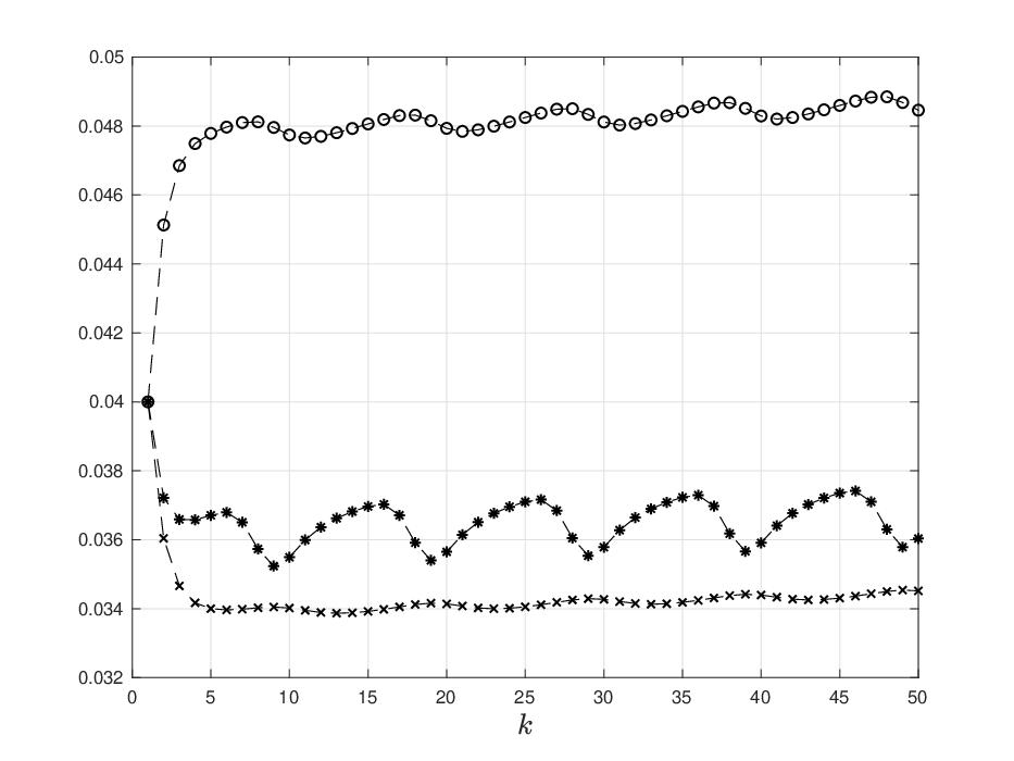
It is clear that we can take the “bounding matrix” $B\in\mathbb{R}^{3\times 3}$ as the matrix with $b_{13}=1$ , and zero in all other entries. It is not difficult to verify that for this $B$ we have that $P(v),Q(v)$ defined in (36) are TP for all $v\in[0,w)$ , with $w:=0.65\exp(-4)$ . Fig. 3 depicts the solution of the system with $\varepsilon=0.0118<w$ and initial condition $x(0)=(2/50)\begin{bmatrix}1&1&1\end{bmatrix}^{\prime}$ . It may be seen that every $x_{i}(k)$ converges to a periodic solution with period $T=10$ .

IV-D Integrating TP Hankel Matrices

Recall that $A\in\mathbb{R}^{n\times n}$ is called a Hankel matrix if for any $i,j,p,q$ with $i+j=p+q$ we have $a_{ij}=a_{pq}$ . For example, for $n=3$ a Hankel matrix has the form

A=\begin{bmatrix}a_{11}&a_{12}&a_{13}\\ a_{12}&a_{13}&a_{23}\\ a_{13}&a_{23}&a_{33}\end{bmatrix}.

Note that a Hankel matrix is in particular symmetric. Our main result in this subsection is that the integral of a time-varying TP Hankel matrix is TP.

Theorem 5

Let $A:[0,1]\to\mathbb{R}^{n\times n}$ be a measurable matrix function such that $A(t)\in L^{\infty}([0,1])$ . Suppose that $A(t)$ is a TP Hankel matrix for almost every $t\in[0,1]$ . Then $\bar{A}$ is TP.

Remark 4

Note that for $n=2$ this implies that if $A:[0,1]\to\mathbb{R}^{2\times 2}$ is a continuous matrix function with $A(t)$ symmetric and TP for all $t\in[0,1]$ then $\bar{A}$ is TP (compare with Example 2).

To prove Thm. 5 we recall several definitions and results. A set of indices $I\subseteq\left\{1,\cdots,n\right\}$ is called an interval if it has the form $I=\{p,p+1,p+2,\dots,q\}$ . A square sub-matrix of a matrix $B\in\mathbb{R}^{n\times n}$ with row indices $I\subseteq\left\{1,\cdots,n\right\}$ and column indices $J\subseteq\left\{1,\cdots,n\right\}$ is called a contiguous sub-matrix if both $I$ and $J$ are intervals.

It is well-known and straightforward to show that the following three conditions are equivalent: (1) $B\in\mathbb{R}^{n\times n}$ is a Hankel matrix; (2) every contiguous sub-matrix of $B$ is a Hankel matrix; (3) every contiguous sub-matrix of $B$ is symmetric.

We can now prove Thm. 5.

Proof:

We start by showing that $\det\bar{A}>0$ . First, note that the function $t\mapsto\det(A(t))$ is measurable (as it is a polynomial in the entries $a_{i,j}(t)$ , $i,j\in\left\{1,\dots,n\right\}$ ) and essentially bounded. Therefore, it is Lebesgue integrable. For $N\in\{1,2,\dots,\}$ , let

B_{N}:=\left\{t\in[0,1]:\det(A(t))\geq N^{-1}\right\}.

Since $A(t)$ is TP for almost every $t\in[0,1]$ and

B_{1}\subseteq B_{2}\subseteq\dots,

the monotone convergence theorem (see e.g. [5]) yields

\lim_{N\rightarrow\infty}\mu(B_{N})=1,

where $\mu$ is the Lebesgue measure on $[0,1]$ . Therefore, there exists $N_{0}\in\mathbb{N}$ such that $\mu(B_{N_{0}})>\frac{1}{2}$ . Markov’s inequality (see e.g. [5]) yields

	$\displaystyle\int_{0}^{1}\left(\det{A(t)}\right)^{\frac{1}{n}}\mathop{}\!\mathrm{d}\mu(t)$	$\displaystyle\geq N_{0}^{-\frac{1}{n}}\mu(B_{N_{0}})$
		$\displaystyle>N_{0}^{-\frac{1}{n}}/2.$		(38)

Since $A(t)$ is Hankel and TP for almost all $t\in[0,1]$ , it is symmetric with positive principal minors, so $A(t)$ is positive-definite for almost all $t\in[0,1]$ . Minkowki’s determinant inequality (see e.g. [12, p. 115]) states that $B\mapsto(\det B)^{\frac{1}{n}}$ is a concave function over the space of semi-positive definite matrices of order $n$ . Thus, by using (IV-D) and Jensen’s inequality (see e.g. [5]) we obtain

	$\displaystyle(\det\bar{A})^{\frac{1}{n}}$	$\displaystyle=\left(\det\int_{0}^{1}A(t)\mathop{}\!\mathrm{d}\mu(t)\right)^{\frac{1}{n}}$
		$\displaystyle\geq\int_{0}^{1}(\det A(t))^{\frac{1}{n}}\mathop{}\!\mathrm{d}\mu(t)$
		$\displaystyle\geq N_{0}^{-\frac{1}{n}}/2,$

so $\det\bar{A}>0$ .

Recall that every contiguous sub-matrix of $A(t)$ is also a TP and Hankel matrix for almost all $t\in[0,1]$ , so the same argument shows that every contiguous minor of $\bar{A}$ is positive. It is well-known [7, Chapter 3] that if all the contiguous minors of a matrix are positive then the matrix is TP, so we conclude that $\bar{A}$ is TP. ∎

The next example demonstrates an application of Remark 4 to a dynamical system.

Example 8

Consider the nonlinear system:

	$\displaystyle x_{1}(k+1)$	$\displaystyle=h_{1}(x_{1}(k))+g(x_{1}(k),x_{2}(k)),$
	$\displaystyle x_{2}(k+1)$	$\displaystyle=h_{2}(x_{2}(k))+g(x_{1}(k),x_{2}(k)),$		(39)

with $h_{1},h_{2},g\in C^{1}$ , whose trajectories evolve on a compact and convex state-space $\Omega\subset\mathbb{R}^{2}$ . Suppose that $\frac{\partial}{\partial x_{1}}g(x_{1},x_{2})=\frac{\partial}{\partial x_{2}}g(x_{1},x_{2})$ for all $x_{1},x_{2}\in\Omega$ (e.g. $g(x_{1},x_{2})=\tanh(x_{1}+x_{2})$ ). Note that this implies that the Jacobian

J(x)=\begin{bmatrix}h_{1}^{\prime}(x_{1})+\frac{\partial}{\partial x_{1}}g(x_{1},x_{2})&\frac{\partial}{\partial x_{2}}g(x_{1},x_{2})\\ \frac{\partial}{\partial x_{1}}g(x_{1},x_{2})&h_{2}^{\prime}(x_{2})+\frac{\partial}{\partial x_{2}}g(x_{1},x_{2})\\ \end{bmatrix}

is symmetric. If $J(x_{1},x_{2})$ is TP for all $(x_{1},x_{2})\in\Omega$ then combining Corollary 1 and Remark 4 implies that any solution of (8) emanating from $\Omega$ converges to an equilibrium point.

V Conclusion

We introduced a new class of positive discrete-time LTV systems called ODTSs of order $p$ . Discrete-time nonlinear systems, whose variational system is an ODTS of order $p$ , have a well-ordered behavior. More precisely, if the map defining the dynamical system is $T$ -periodic then every solution either leaves any compact set or converges to a $pT$ -periodic solution, i.e. a subharmonic solution. This is important because, as noted by Smith [30], “…in the class of all discrete dynamical systems, we do not know so many special classes which have relatively simple dynamics.”

The ODTS framework requires establishing that certain line integrals of the Jacobian of the time-varying nonlinear system are oscillatory matrices. This is non-trivial, as the sum of two oscillatory matrices is not necessarily oscillatory, and this naturally extends to integrals. We derived several sufficient conditions guaranteeing that the line integral of a matrix is oscillatory (or TP).

Topics for further research include the following. First, extending the oscillatory framework to other dynamical models e.g. systems with time-delays or discretized PDEs. Second, cooperative discrete-time systems arise frequently as the Poincaré maps of continuous-time systems. It may be of interest to explore the implications of oscillatory Poincaré maps. Third, it may be of interest to generalize the ODTS framework to discrete-time systems with control inputs, as was done for continuous-time monotone systems in [2].

Appendix

Proof:

Let $z:=D_{\pm}(x-y)$ . Then (14) implies that $v:=D_{\pm}Pz\ll 0$ . Thus, the vector $Pz=D_{\pm}v$ is alternating, with

(Pz)_{1}=v_{1}<0.

Applying the VDP (6) yields

n-1=s^{-}(Pz)\leq s^{-}(z).

Thus, $s^{-}(z)=n-1$ , i.e. $z$ is alternating. Recall that if a matrix $H$ is TN, and non-singular and $s^{-}(Hq)=s^{-}(q)$ for some $q\in\mathbb{R}^{n}\setminus\{0\}$ then the first non-zero entry in $Hq$ and the first non-zero entry in $q$ have the same sign [9, p. 254]. Since $s^{-}(Pz)=s^{-}(z)=n-1$ , and $(Pz)_{1}<0$ , the first non-zero entry of $z$ is negative. Since $z$ is alternating this implies that $D_{\pm}z\ll 0$ , and this completes the proof. ∎

References

[1] R. Alseidi, M. Margaliot, and J. Garloff, “On the spectral properties of nonsingular matrices that are strictly sign-regular for some order with applications to totally positive discrete-time systems,” J. Math. Anal. Appl., vol. 474, pp. 524–543, 2019.
[2] D. Angeli and E. D. Sontag, “Monotone control systems,” IEEE Trans. Automat. Control, vol. 48, pp. 1684–1698, 2003.
[3] T. Ben-Avraham, G. Sharon, Y. Zarai, and M. Margaliot, “Dynamical systems with a cyclic sign variation diminishing property,” IEEE Trans. Automat. Control, 2019, to appear. [Online]. Available: http://arxiv.org/abs/1807.02779
[4] R. A. Blythe and M. R. Evans, “Nonequilibrium steady states of matrix-product form: a solver’s guide,” J. Phys. A: Math. Gen., vol. 40, no. 46, pp. R333–R441, 2007.
[5] V. I. Bogachev, Measure Theory. Berlin Heidelberg: Springer-Verlag, 2007, vol. 1.
[6] A. Csikasz-Nagy, L. Cardelli, and O. S. Soyer, “Response dynamics of phosphorelays suggest their potential utility in cell signaling,” J. Royal Society Interface, vol. 8, pp. 480–488, 2011.
[7] S. M. Fallat and C. R. Johnson, Totally Nonnegative Matrices. Princeton, NJ: Princeton University Press, 2011.
[8] L. Farina and S. Rinaldi, Positive Linear Systems: Theory and Applications. John Wiley, 2000.
[9] F. R. Gantmacher and M. G. Krein, Oscillation Matrices and Kernels and Small Vibrations of Mechanical Systems. Providence, RI: American Mathematical Society, 2002, translation based on the 1941 Russian original.
[10] J. Garloff, “Intervals of almost totally positive matrices,” Linear Algebra Appl., vol. 363, pp. 103–108, 2003.
[11] M. W. Hirsch and H. L. Smith, “Competitive and cooperative systems: A mini-review,” in Positive Systems, L. Benvenuti, A. De Santis, and L. Farina, Eds. Berlin, Heidelberg: Springer, 2003, pp. 183–190.
[12] M. Marcus and H. Minc, A Survey of Matrix Theory and Matrix Inequalities. Courier Corporation, 1992, vol. 14.
[13] M. Margaliot, L. Grüne, and T. Kriecherbauer, “Entrainment in the master equation,” Royal Society Open Science, vol. 5, no. 4, p. 171582, 2018.
[14] M. Margaliot, L. Grüne, and T. Kriecherbauer, “Entrainment in the master equation,” Royal Society Open Science, vol. 5, no. 4, p. 172157, 2018.
[15] M. Margaliot, E. D. Sontag, and T. Tuller, “Entrainment to periodic initiation and transition rates in a computational model for gene translation,” PLOS ONE, vol. 9, no. 5, p. e96039, 2014.
[16] M. Margaliot and E. D. Sontag, “Revisiting totally positive differential systems: A tutorial and new results,” Automatica, vol. 101, pp. 1–14, 2019.
[17] I. Nanikashvili, Y. Zarai, A. Ovseevich, T. Tuller, and M. Margaliot, “Networks of ribosome flow models for modeling and analyzing intracellular traffic,” Sci. Rep., vol. 9, no. 1703, 2019.
[18] A. Pinkus, Totally Positive Matrices. Cambridge, UK: Cambridge University Press, 2010.
[19] G. Poker, Y. Zarai, M. Margaliot, and T. Tuller, “Maximizing protein translation rate in the nonhomogeneous ribosome flow model: A convex optimization approach,” J. Royal Society Interface, vol. 11, no. 100, p. 20140713, 2014.
[20] A. Rantzer and M. E. Valcher, “A tutorial on positive systems and large scale control,” in Proc. 57th IEEE Conf. on Decision and Control, Miami Beach, FL, USA, 2018, pp. 3686–3697.
[21] A. Raveh, M. Margaliot, E. D. Sontag, and T. Tuller, “A model for competition for ribosomes in the cell,” J. Royal Society Interface, vol. 13, no. 116, 2016.
[22] S. Reuveni, I. Meilijson, M. Kupiec, E. Ruppin, and T. Tuller, “Genome-scale analysis of translation elongation with a ribosome flow model,” PLOS Computational Biology, vol. 7, p. e1002127, 2011.
[23] G. Russo, M. di Bernardo, and E. D. Sontag, “Global entrainment of transcriptional systems to periodic inputs,” PLOS Computational Biology, vol. 6, p. e1000739, 2010.
[24] I. W. Sandberg, “On the mathematical foundations of compartmental analysis in biology, medicine, and ecology,” IEEE Trans. Circuits and Systems, vol. 25, no. 5, pp. 273–279, 1978.
[25] B. Schwarz, “Totally positive differential systems,” Pacific J. Math., vol. 32, no. 1, pp. 203–229, 1970.
[26] R. Shorten, F. Wirth, and D. Leith, “A positive systems model of TCP-like congestion control: asymptotic results,” IEEE/ACM Trans. Networking, vol. 14, no. 3, pp. 616–629, 2006.
[27] J. Smillie, “Competitive and cooperative tridiagonal systems of differential equations,” SIAM J. Math. Anal., vol. 15, pp. 530–534, 1984.
[28] H. L. Smith, “Periodic tridiagonal competitive and cooperative systems of differential equations,” SIAM J. Math. Anal., vol. 22, no. 4, pp. 1102–1109, 1991.
[29] H. L. Smith, Monotone Dynamical Systems: An Introduction to the Theory of Competitive and Cooperative Systems, ser. Mathematical Surveys and Monographs. Providence, RI: Amer. Math. Soc., 1995, vol. 41.
[30] H. L. Smith, “Planar competitive and cooperative difference equations,” J. Differ. Equ. Appl., vol. 3, no. 5-6, pp. 335–357, 1998.
[31] H. L. Smith, “Monotone dynamical systems: Reflections on new advances & applications,” Discrete and Continuous Dynamical Systems, vol. 37, pp. 485–504, 2017.
[32] P. Takáč, “Linearly stable subharmonic orbits in strongly monotone time-periodic dynamical systems,” Proc. AMS, vol. 115, no. 3, pp. 691–698, 1992.
[33] A. M. Whitney, “A reduction theorem for totally positive matrices,” J. d’Analyse Mathématique, vol. 2, no. 1, pp. 88–92, 1952.
[34] Y. Zarai, M. Margaliot, and T. Tuller, “On the ribosomal density that maximizes protein translation rate,” PLOS ONE, vol. 11, no. 11, pp. 1–26, 2016.

Entrainment to Subharmonic Trajectories in Oscillatory Discrete-Time SystemsThanks: An abridged version of this paper has been submitted to the 27th Mediterranean Conference on Control and Automation (MED 2019).

Abstract

Index Terms:

I Introduction

II Preliminaries

II-A Totally Positive Discrete-Time Systems

Assumption 1

Assumption 2

Theorem 1

Corollary 1

Lemma 1

Example 1

Example 2

Example 3

III Oscillatory Discrete-Time Systems

Definition 1

Assumption 3

Theorem 2

Remark 1

Remark 2

Proof:

Remark 3

IV Conditions guaranteeing that a matrix line integral is oscillatory

IV-A Discretizing nonlinear tridiagonal strongly cooperative systems

Lemma 2

Proof:

Example 4

Example 5

IV-B The case of strictly monotone scalar nonlinearities

Theorem 3

Proof:

Example 6

Problem 1

IV-C Sufficient condition based on the checkerboard partial order

Definition 2

Theorem 4

Proof:

Corollary 2

Proof:

Example 7

IV-D Integrating TP Hankel Matrices

Theorem 5

Remark 4

Proof:

Example 8

V Conclusion

Appendix

Proof:

References

Entrainment to Subharmonic Trajectories in
Oscillatory Discrete-Time SystemsThanks: An abridged version of this paper has been submitted to the 27th Mediterranean Conference on Control and Automation (MED 2019).