Energy Efficient Node Deployment in Wireless Ad-hoc Sensor Networks

Recent developments in wireless communications, digital electronics and computational power have enabled a large number of applications of wireless ad-hoc sensor networks (WASNs) in various fields such as agriculture, industry and military. In a general WASN, spatially dispersed and dedicated sensors collect data, e.g. temperature, sound, pressure and radio signals from the physical environment, and then forward the gathered information to one or more fusion centers (FCs) via wireless communications.

In order to collect accurate data from the physical surroundings, high sensing quality or sensitivity is required. In general, sensing quality diminishes as the distance between the sensor and target point increases [1, 3, 4, 2, 5, 6]. Thus, two distance-dependent measures, i.e., sensing coverage [1, 7, 8, 9, 10] and sensing uncertainty [2, 15, 14, 16, 12, 11, 13] are widely studied in the literature to evaluate the sensing quality. In the binary coverage model [1, 7, 8, 9, 10], each sensor node can only detect the events within the sensing radius $R_{s}$. Then, sensing coverage represents the percentage of events that is covered by at least one sensor [1, 7, 8, 9]. But when the number of sensors is large enough, such that the full coverage can be achieved, coverage degree [10], i.e., the minimum number of sensors that any event can be detected by, is a better sensing quality measure. Another common model, centroidal Voronoi tessellation, formulates the sensing quality as a source coding problem with sensing uncertainty as its distortion [2, 15, 14, 16, 12, 11, 13].

Energy efficiency is another key metric in WASNs as it is inconvenient or even infeasible to recharge the batteries of numerous and densely deployed sensors. In general, wireless communication, sensing and data processing are three primary energy consumption components of a node. However, in many WASN applications, wireless communication among nodes is more power hungry compared to other components [17, 18]. Therefore, wireless communication dominates the node energy consumption in practice.

There are four primary energy saving methods for WASNs in the literature: (1) topology control [19, 20], in which unnecessary energy consumption is reduced by properly switching the nodes’ states (sleeping or working); (2) clustering [22, 21] which is used to balance the energy consumption among nodes in one-hop communication models by iteratively selecting cluster heads; (3) energy-efficient routing [23, 24, 25], a widely used method that attempts to find the optimal routing paths to forward data to FCs while the communication cost between two nodes are held fixed; and (4) deployment optimization that plays an important role in the energy consumption of WASNs since the communication cost between two nodes depends on their distance. Our previous works [26, 27] proposed Lloyd-like algorithms to save communication energy in homogeneous and heterogeneous WASNs by optimizing the node deployment. Nonetheless, a pre-existing network infrastructure, which only includes two-hop communications, is a basic assumption in [26, 27]. Compared to one-hop and two-hop communications, the generalized multi-hop communications can, on average, reduce the transmission distance and save more energy. However, to the best of our knowledge, the optimal node deployment with generalized multi-hop communications in WASNs is still an open problem.

In this paper, we study the node deployment problem in WASNs with arbitrary multi-hop routing algorithms. Our primary goal is to find the optimal FC and sensor deployment to minimize both sensing uncertainty and total energy consumption of the network. By deriving the routing-dependent necessary conditions of the optimal deployments in such WASNs, we design a Lloyd-like algorithm to deploy nodes.

The rest of this paper is organized as follows: In Section II, we introduce the system model and problem formulation. In Section III, we study the optimal FC and sensor deployment for a given routing algorithm. A numerical algorithm is proposed in Section IV to optimize the node deployment. Section V presents the experimental results and Section VI concludes the paper.

We consider a wireless ad-hoc sensor network consisting of $M$ FCs and $N$ sensors over a target region $\Omega\in\mathbb{R}^{2}$. For convenience, we define $\mathcal{I}_{S}=\{1,\dots,N\}$ to be the set of node indices for sensors and $\mathcal{I}_{F}=\{N+1,\dots,N+M\}$ to be the set of node indices for FCs. When $i\in\mathcal{I}_{S}$, Node $i$ refers to Sensor $i$; however, when $i\in\mathcal{I}_{F}$, Node $i$ refers to FC $(i-N)$. Let $\mathbf{P}=(p_{1},\dots,p_{N},p_{N+1},\dots,p_{N+M})^{T}\in\mathbb{R}^{(N+M)\times 2}$ be the node deployment, where $p_{i}\in\Omega$ is Node $i$’s location. Throughout this paper, we assume that each event is sensed by only one sensor. Therefore, for each node deployment $\mathbf{P}$, there exists a cell partitioning $\mathbf{W}=(W_{1},\dots,W_{N})^{T}$ comprised of $N$ disjoint subsets of $\mathbb{R}^{2}$ whose union is $\Omega$, and each sensor, say $i$, only monitors the events occurred in the cell $W_{i}\subseteq\Omega$. The spatial density function that reflects the frequency of random events taking place over the target region $\Omega$ is denoted via a continuous and differentiable function $f(\omega):\Omega\to\mathbb{R}^{+}$. Let $\mathbf{\Gamma}(\mathbf{W})=\left(\Gamma_{1}(\mathbf{W}),\dots,\Gamma_{N}(\mathbf{W})\right)^{T}\in\mathbb{R}^{N}$ where $\Gamma_{i}(\mathbf{W})$ is the amount of data generated at Node (Sensor) $i$ in the unit time. Since Sensor $i$ detects the events in the region $W_{i}$, $\Gamma_{i}(\mathbf{W})$ is proportional to the volume of $W_{i}$, i.e., $\Gamma_{i}(\mathbf{W})=\kappa\int_{W_{i}}f(\omega)d\omega$ where $\kappa$ is a constant, [26].

According to [23], this WASN can be modeled as a directed acyclic graph $\mathcal{G}(\mathcal{I}_{S}\bigcup\mathcal{I}_{F},\mathcal{E})$ where $\mathcal{E}$ is the set of directed links $(n,k)$ such that $n\in\mathcal{I}_{S}$ and $k\in\mathcal{I}_{S}\bigcup\mathcal{I}_{F}$. In particular, sensors and FCs are source nodes and sink nodes of this network, respectively, and there is no cycle in the flow network since each cycle can be eliminated by reducing the flows along the cycle without influencing the in-flow and out-flow links to that cycle. We define $\mathbf{F}=[F_{i,j}]_{N\times(N+M)}$ to be the flow matrix, where $F_{i,j}$ is the amount of data transmitted through the link $(i,j)$ in the unit time. Since $\mathbf{F}$ depends on the cell partitioning $\mathbf{W}$, we can define the normalized flow matrix as follows:

Since the flow $F_{i,j}$ can be determined by the cell partitioning $\mathbf{W}$ and normalized flow matrix $\mathbf{S}$, in the remaining of this paper we use $\mathbf{F}(\mathbf{W},\mathbf{S})$ instead of $\mathbf{F}$. Let $F_{i}(\mathbf{W},\mathbf{S})\triangleq\sum_{j=1}^{N+M}F_{i,j}(\mathbf{W},\mathbf{S})$ be the total flow originated from Node $i$. Since the in-flow to each sensor, say $i$, should be equal to the out-flow, we have $\sum_{j=1}^{N}F_{j,i}(\mathbf{W},\mathbf{S})+\Gamma_{i}(\mathbf{W})=\sum_{j=1}^{N+M}F_{i,j}(\mathbf{W},\mathbf{S}).$ In what follows, we provide an example to elucidate how to calculate $F(\mathbf{W},\mathbf{S})$ in terms of $\mathbf{W}$ and $\mathbf{S}$.

Example 1. We consider a WASN with three sensor nodes and one FC, i.e., $N=3$ and $M=1$. The parameter $\kappa$ is set to $4$. For a cell partitioning $\mathbf{W}$ with cell volumes $v_{1}(W)=v_{2}(W)=0.25$, $v_{3}(W)=0.5$, and the normalized flow matrix $\mathbf{S}=\begin{array}[]{rccccl}\hbox{\multirowsetup$\left.\vbox{\vrule height=0.0pt,width=0.0pt}\textnormal{}\right[$}&0&0.5&0.5&0&\hbox{\multirowsetup$\left]\vbox{\vrule height=0.0pt,width=0.0pt}\textnormal{}\right.$}\\ &0&0&0.4&0.6&\\ &0&0&0&1&\\ \end{array}$, the corresponding flow network is illustrated in Fig. 1.

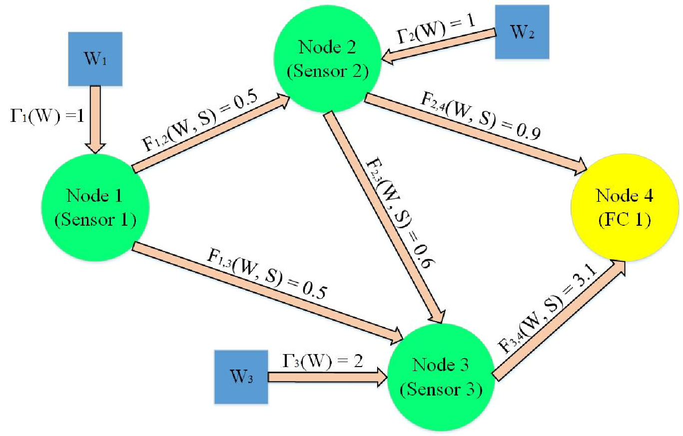
The amount of data generated from each sensor node can be calculated as: $\Gamma_{1}(\mathbf{W})\!=\!\kappa v_{1}(\mathbf{W})\!=\!1$, $\Gamma_{2}(\mathbf{W})\!=\!\kappa v_{2}(\mathbf{W})\!=\!1$, and $\Gamma_{3}(\mathbf{W})\!=\!\kappa v_{3}(\mathbf{W})\!=\!2$. As a leaf node, Sensor 1 does not receive data from any other sensor nodes, and only transmits its sensed data; thus, $F_{1}(\mathbf{W},\mathbf{S})\!=\!\Gamma_{1}(\mathbf{W})\!=\!1$. The flows from Sensor $1$ are then $F_{1,2}(\mathbf{W},\mathbf{S})\!=\!s_{1,2}\!\times\!F_{1}(\mathbf{W},\mathbf{S})\!=\!0.5$ and $F_{1,3}(\mathbf{W},\mathbf{S})\!=\!s_{1,3}\!\times\!F_{1}(\mathbf{W},\mathbf{S})\!=\!0.5$, respectively. Sensor $2$’s flows come from $F_{1,2}(\mathbf{W},\mathbf{S})$ and the data gathered from the region $W_{2}$. Hence, $F_{2}(\mathbf{W},\mathbf{S})\!=\!\Gamma_{2}(\mathbf{W})\!+\!F_{1,2}(\mathbf{W},\mathbf{S})\!=\!1.5$. Therefore, the flows from Sensor $2$ are $F_{2,3}(\mathbf{W},\mathbf{S})\!=\!s_{2,3}\!\times\!F_{2}(\mathbf{W},\mathbf{S})\!=\!0.6$ and $F_{2,4}(\mathbf{W},\mathbf{S})\!=\!s_{2,4}\!\times\!F_{2}(\mathbf{W},\mathbf{S})\!=\!0.9$. Similarly, for Sensor $3$, we have $F_{3}(\mathbf{W},\mathbf{S})\!=\!\Gamma_{3}(\mathbf{W})\!+\!F_{1,3}(\mathbf{W},\mathbf{S})\!+\!F_{2,3}(\mathbf{W},\mathbf{S})\!=\!3.1$; hence, the unique flow from Sensor $3$ is $F_{3,4}(\mathbf{W},\mathbf{S})\!=\!s_{3,4}\times F_{3}(\mathbf{W},\mathbf{S})\!=\!3.1$.

Now, we have enough materials to formulate the energy consumption in a WASN. In general, FCs are equipped with reliable energy sources and their energy consumption is not the main concern. In what follows, we focus on the sensor energy consumption. The average power consumption (Watts) through link $(i,j)$ consists of two components: average-transmitter-power, $\overline{\mathcal{P}}^{T}_{i,j}$, and average-receiver-power, $\overline{\mathcal{P}}^{R}_{i,j}$. Sensor $i$’s average-transmitter-power through link $(i,j)$ can be expressed as $\overline{\mathcal{P}}^{T}_{i,j}=\mathcal{P}^{T}_{i,j}\times r_{i,j}$, where $\mathcal{P}^{T}_{i,j}$ is Sensor $i$’s instant-transmitter-power through link $(i,j)$, and $r_{i,j}$ is the link-busy-ratio, i.e., the percentage of time that data is going through link $(i,j)$. To achieve a reliable communication between two nodes, the instant-transmission-power (Joules/second) required for Node $i$ to transmit data to Node $j$ should be set to $\mathcal{P}^{T}_{i,j}=\xi_{i,j}||p_{i}-p_{j}||^{\alpha}$, where $||.||$ denotes the Euclidean distance, $\alpha$ is the path-loss parameter, $\xi_{i,j}$ is a constant determined by Node $i$’s antenna gain, Node $j$’s antenna gain, and Node $j$’s SNR threshold. In this paper, we consider free-space path-loss, i.e., $\alpha=2$ and homogeneous sensors and FCs, i.e., $\xi_{i,j}=\xi$. Therefore, the instant-transmitter-power through link $(i,j)$ is modeled as $\mathcal{P}^{T}_{i,j}=\xi||p_{i}-p_{j}||^{2}$. It is reasonable to assume that the link $(i,j)$ has idle time, and it is busy only when there is data to transmit from Node $i$ to Node $j$. Hence, link $(i,j)$’s link-busy-ratio can be written as $\frac{F_{i,j}(\mathbf{W},\mathbf{S})\times T/\zeta_{i,j}}{T}=\frac{F_{i,j}(\mathbf{W},\mathbf{S})}{\zeta_{i,j}}$, where $\zeta_{i,j}$ is the instant-data-rate through link $(i,j)$ which is determined by the bandwidth of $(i,j)$. In this paper, we assume that all links have the same bandwidth, i.e., $\zeta_{i,j}=\zeta$. Therefore, Sensor $i$’s average-transmitter-power through link $(i,j)$ can be rewritten as $\overline{\mathcal{P}}^{T}_{i,j}=\beta||p_{i}-p_{j}||^{2}F_{i,j}(\mathbf{W},\mathbf{S})$, where $\beta=\frac{\xi}{\zeta}$. According to [28], Sensor $j$’s average-receiver-power through link $(i,j)$ can be modeled as $\overline{\mathcal{P}}^{R}_{i,j}=\rho F_{i,j}(\mathbf{W},\mathbf{S})$, where $\rho$ is a constant coefficient for receiving data. In sum, the average power consumption over link $(i,j)$ can be written as

and the total power consumption can be written as

According to [2, 15, 14, 16, 12, 11, 13], for a given node deployment $\mathbf{P}$ and cell partitioning $\mathbf{W}$, the sensing uncertainty can be formulated as:

Taking sensing uncertainty and energy consumption into consideration, the objective (cost) function is then defined as the Lagrangian function of Eqs. (3) and (4):

where $\lambda\geq 0$ is the Lagrangian multiplier. Our main goal in this paper is to minimize the cost function defined in (5) over the node deployment $\mathbf{P}$, cell partitioning $\mathbf{W}$, and the normalized flow matrix $\mathbf{S}$.

In this section, we study the optimality conditions for node deployment $\mathbf{P}$, cell partitioning $\mathbf{W}$ and the normalized flow matrix $\mathbf{S}$ to minimize the objective function defined in (5). Let

be the Link $(i,j)$’s energy cost (Joules/bit). Without loss of generality, we assume that Sensor $i$’s sensing data goes through $K_{i}$ paths $\{L^{(i)}_{k}(\mathbf{S})\}_{k\in\{1,\dots,K_{i}\}}$, where $L^{(i)}_{k}(\mathbf{S})=l^{(i)}_{k,0}\to l^{(i)}_{k,1}\to\cdots\to l^{(i)}_{k,J^{(i)}_{k}}$, $l^{(i)}_{k,0}=i$, $l^{(i)}_{k,J^{(i)}_{k}}\in\mathcal{I}_{F}$, and $J^{(i)}_{k}$ is the number of nodes on the $k$-th path except Node $i$. Then, the data rate (bit/s) and the path cost (Joules/bit) corresponding to the $k$-th path can be written as

and

respectively. Note that $\sum_{k}\mu_{k}^{(i)}(\mathbf{W},\mathbf{S})=F_{i}(\mathbf{W},\mathbf{S})$ which means the data from Node $i$ eventually reach a FC. Sensor $i$’s power coefficient, denoted as $g_{i}(\mathbf{P},\mathbf{S})$, is then defined to be the energy consumption (Joules/bit) for transmitting $1$ bit data from Sensor $i$ to the FCs, i.e, we have²² 2 The term $F_{i}(\mathbf{W},\mathbf{S})$ is canceled in Eq. (9), indicating that power coefficient $g_{i}(\mathbf{P},\mathbf{S})$ is independent of $\mathbf{W}$.:

In what follows, we provide an example to clarify how to calculate the sensor power coefficients.

Example 2. Consider the WASN described in Fig. 1, and let $\mathbf{P}=((0,0),(0,1),(1,0),(1,1))$, $\beta\!=\!1$ and $\rho\!=\!1$. We aim to find Sensor 1’s power coefficient $g_{1}(\mathbf{P},\mathbf{S})$. The link energy costs for this network can be calculated as $e_{1,2}(\mathbf{P})=e_{1,3}(\mathbf{P})\!=\!2$, $e_{2,3}(\mathbf{P})\!=\!3$, and $e_{2,4}(\mathbf{P})\!=\!e_{3,4}(\mathbf{P})\!=\!1$. Note that Sensor $1$’s data goes through the following 3 paths: $L^{(1)}_{1}(\mathbf{S})\!=\!1\!\to\!2\!\to\!4$, $L^{(1)}_{2}(\mathbf{S})\!=\!1\!\to\!3\!\to\!4$, and $L^{(1)}_{3}(\mathbf{S})\!=\!1\!\to\!2\!\to\!3\!\to\!4$. The data rate through the above paths are, respectively, $\mu_{1}^{(1)}(\mathbf{W},\mathbf{S})\!=\!F_{1}(\mathbf{W},\mathbf{S})\!\times\!s_{1,2}\!\times\!s_{2,4}\!=\!0.3F_{1}(\mathbf{W},\mathbf{S})$, $\mu_{2}^{(1)}(\mathbf{W},\mathbf{S})\!=\!F_{1}(\mathbf{W},\mathbf{S})\!\times\!s_{1,3}\!\times\!s_{3,4}\!=\!0.5F_{1}(\mathbf{W},\mathbf{S})$, and $\mu_{3}^{(1)}(\mathbf{W},\mathbf{S})\!=\!F_{1}(\mathbf{W},\mathbf{S})\!\times\!s_{1,2}\!\times\!s_{2,3}\!\times\!s_{3,4}\!=\!0.2F_{1}(\mathbf{W},\mathbf{S})$. Moreover, we can calculate the path costs using Eq. (8) as follows: $\overline{e}^{(1)}_{1}(\mathbf{P})=e_{1,2}(\mathbf{P})+e_{2,4}(\mathbf{P})=3$, $\overline{e}^{(1)}_{2}(\mathbf{P})=e_{1,3}(\mathbf{P})+e_{3,4}(\mathbf{P})=3$, and $\overline{e}^{(1)}_{3}(\mathbf{P})=e_{1,2}(\mathbf{P})+e_{2,3}(\mathbf{P})+e_{3,4}(\mathbf{P})=6$. Then, Sensor $1$’s power coefficient is $g_{1}(\mathbf{P},\mathbf{S})=0.3\times 3+0.5\times 3+0.2\times 6=3.6$.

Note that the average power consumption for transmitting Sensor $i$’s data is $g_{i}(\mathbf{P},\mathbf{S})\Gamma_{i}(\mathbf{W})\!=\!g_{i}(\mathbf{P},\mathbf{S})\kappa\int_{\mathbf{W}_{i}}\!\!f(\omega)d\omega$. Thus, the total power consumption (3) can be rewritten as:

Therefore, the cost function in (5) can be rewritten as:

Given the node deployment $\mathbf{P}$ and normalized flow matrix $\mathbf{S}$, the optimal cell partitioning, also referred to as power diagrams in [30], is equal to:

Moreover, given the link costs $\{e_{ij}(\mathbf{P})\}$s and generated sensing data rates $\{\Gamma_{i}(\mathbf{W})\}$s, the total power consumption can be minimized by Bellman-Ford Algorithm [24, 25]. For convenience, we represent the functionality of Bellman-Ford Algorithm by $\mathcal{R}(\mathbf{P},\mathbf{W})$, where $\mathbf{P}$ and $\mathbf{W}$ are inputs and $\mathbf{S}$ is the output, i.e., $\mathcal{R}(\mathbf{P},\mathbf{W})=\arg\min_{\mathbf{S}}\overline{\mathcal{P}}(\mathbf{P},\mathbf{W},\mathbf{S})$. Since sensing uncertainty $\mathcal{H}(\mathbf{P},\mathbf{W})$ is independent of $\mathbf{S}$, we have:

The optimal flow matrix for the given $\mathbf{P}$ and $\mathbf{W}$ is then $\mathbf{F}(\mathbf{W},\mathcal{R}(\mathbf{P},\mathbf{W}))$. The following theorem provides the necessary conditions for the optimal deployment.

The proof of Theorem 1 is provided in Appendix A. Let $\mathcal{N}^{P}_{i}(\mathbf{S})\triangleq\{j|F_{j,i}(\mathbf{W},\mathbf{S})>0\}$ be the set of Node $i$’s predecessors, and $\mathcal{N}^{S}_{i}(\mathbf{S})\triangleq\{j|F_{i,j}(\mathbf{W},\mathbf{S})>0\}$ be the set of Node $i$’s successors. Hence, Eqs. (14) and (15) can be simplified as

for each $i\in\mathcal{I}_{S}$, and

for each $i\in\mathcal{I}_{F}$, respectively. In other words, Sensor $i$’s optimal location is a linear combination of its geometric centroid, predecessors, and successors while FC $j$’s optimal location is a linear combination of its predecessors.

Before introducing our new Routing-aware Lloyd (RL) Algorithm to solve the deployment problem, we quickly review Lloyd Algorithm [29]. Lloyd Algorithm iterates between two steps: (i) Voronoi partitioning and (ii) Moving each node to the geometric centroid of its corresponding Voronoi region. Based on Lloyd Algorithm, we use the necessary conditions in Theorem 1 to design RL Algorithm and optimize the node deployment in WASNs. Starting with a random initialization for node deployment $\mathbf{P}$ in the target region $\Omega$, first, we design a quantizer with $N$ ($M$) points for the sensor density function and place the sensors (FCs) on the corresponding centroids to encourage an even distribution of sensors among FCs and account for a possibly poor initial node deployment. RL Algorithm then iterates between three steps: (i) Update node locations according to Eqs. (14) and (15); (ii) Run Bellman-Ford Algorithm to obtain the flow matrix $\mathbf{F}(\mathbf{P},\mathbf{W})$ and update the normalized flow matrix $\mathbf{S}$ and sensor power coefficients $g_{i}(\mathbf{P},\mathbf{S})$; and (iii) Calculate the cell partitioning according to Eq. (16) and update the value of volumes $v_{n}$ and centroids $c_{n}$. The algorithm continues until the stop criterion is satisfied. The details of RL Algorithm is provided in Algorithm 1.

The proof of Theorem 2 is provided in Appendix B.

In this section, we provide the experimental results for a WASN including 4 FCs and 40 sensors. To make a fair comparison, we use the same target region and density function as in [26, 27], i.e., $\Omega=[0,10]^{2}$ and $f(\omega)=\frac{1}{\int_{\Omega}dA}=0.01$. Other parameters are set as follows: $\beta=1$, $\rho=0.1$, $\kappa=1$, $\epsilon=10^{-6}$.

Note that there is no existing work except our previous paper [26] considering both sensing uncertainty and energy consumption. Bellman-Ford Algorithm [24, 25] is the best routing algorithm to minimize the total energy consumption, but it does not take node deployment into account. To compare with Bellman-Ford Algorithm, we apply random deployment and Lloyd Algorithm [29] for the node deployment part. Random deployment + Bellman-Ford (RBF) employs Bellman-Ford Algorithm on 100 random node deployments and selects the best one. Similarly, Lloyd + Bellman-Ford (LBF) first applies Lloyd Algorithm to both FCs and Sensors to obtain a node deployment with small cost, and then employs Bellman-Ford Algorithm to reduce the average power. Furthermore, we compare RL with CL [26] which combines two Lloyd-like algorithms to optimize the node deployment with one-hop communications.

Performance comparisons³³ 3 To better exhibit the performance of LBF, CL, RL, we do not show the results of RBF with excessive powers ($\overline{\mathcal{P}}>6$) in Fig. 2. for different values of $\lambda\in\left\{0,0.05,0.15,0.25,0.5,1,1.5,2,3,4,5,7,10,16\right\}$ are provided in Fig. 2. Note that CL and RL can adjust the node deployment in terms of the Lagrangian multiplier $\lambda$ while RBF and LBF are independent of $\lambda$. In particular, since LBF determines the node deployment by Lloyd Algorithm before employing Bellman-Ford Algorithm, LBF’s performance is almost independent of the initial deployments, and its experimental results in Fig. 2 converge to a point with small sensing uncertainty but large power consumption. Overall, the proposed RL algorithm saves more energy or reduces more sensing uncertainty compared to other algorithms. It also provides a trade-off between the average power and sensing uncertainty.

The node deployments of the four algorithms (RBF, LBF, CL, and RL) in the WASN with $\lambda=0.25$ are illustrated in Figs. 3a, 3b, 3c, and 3d. FCs and sensors are denoted by five-pointed stars and circles, respectively. Flows are denoted by black dotted lines. As shown in Fig. 3, cell partitions in LBF, CL and RL algorithms tend to have similar shapes; however, RBF does not result in a similar pattern. Moreover, sensors in Fig. 3b are placed on top of their corresponding centroids while sensors in Fig. 3c are placed between their corresponding FC and centroid. However, in Fig. 3d, location of each sensor depends on its centroid, predecessors, and successors, as provided in Theorem 1. Note that in Figs. 3b, 3c and 3d, sensors inside each cluster tend to be close to each other with their FC in the middle; however, the same relationship does not appear in Fig. 3a. Besides, CL only uses one-hop communications, i.e., sensors are directly connected to the FC while other algorithms utilize multi-hop communications to reduce the average power. The corresponding cost function given $\lambda=0.25$ for RBF, LBF, CL, and RL are, respectively, $1.87$, $1.25$, $1.17$, $1.01$; thus, our RL Algorithm achieves a lower cost function and outperforms other algorithms.

In this paper, we formulated the node deployment in WASNs as an optimization problem to make a trade-off between sensing uncertainty and energy consumption. The necessary conditions for the optimal deployment imply that each sensor location should be a linear combination of its centroid, predecessors and successors. Based on these necessary conditions, we proposed a Lloyd-like algorithm to minimize the total cost. Our experimental results show that the proposed algorithm significantly reduces both sensing uncertainty and energy consumption. Although we only considered Bellman-Ford Algorithm as the routing algorithm in this paper, the proposed system model in Section II can be applied to arbitrary routing algorithms, such as Flow Augmentation Algorithm [23] (a network lifetime maximization routing algorithm). The optimal deployment with maximum network lifetime will be our future work.

References

- [1] S. Meguerdichian, F. Koushanfar, M. Potkinjak, and M. B. Srivastava, “Coverage Problems in Wireless Ad-hoc Sensor Networks,” IEEE Int. Conf. Comput. Commun., Apr. 2001.
- [2] A. Breitenmoser, M. Schwager, J. C. Metzger, R. Siegwart, and D. Rus, “Voronoi coverage of non-convex environments with a group of networked robots,” IEEE Int. Conf. Robot. Autom., 2010.
- [3] S. Meguerdichian, F. Koushanfar, G. Qu, and M. Potkonjak, “Exposure in wireless ad-hoc sensor networks”, ACM Int. Conf. Mobile Comput. Netw., 2001.
- [4] A. Gusrialdi and L. Zeng, “Distributed Deployment Algorithms for Robotic Visual Sensor Networks in Non-Convex Environment”, IEEE Int. Conf. Netw., Sens. Control, 2011.
- [5] T. S. Helal, P. Mozumdar, and L. Akter, “Evaluating the Performance of Optimal Control based Sensor Deployment Algorithms for Realistic Terrain Model,” IEEE Int. Conf. Elect. Comput. Eng., 2014.
- [6] L. Yang, J. Liang, and W. Liu, “Radar sensor (RS) deployment for multi-target detection”, IEEE Int. Conf. Wireless Commun. Signal Process., Oct. 2014.
- [7] M. R. Senouci and A. Mellouk, “Localized Movement-Assisted Sensor Deployment Algorithm for Hole Detection and Healing,” IEEE Trans. Parallel Distrib. Syst., vol. 25, no. 5, pp. 1267-1276, May 2014.
- [8] Y. Zou and K. Chakrabarty, “Sensor deployment and target localization in distributed sensor networks,” ACM Trans. Embedded Comput. Syst., vol. 3, no. 1, pp. 61¨C91, 2004.
- [9] Y. Yoon and Y.-H. Kim, “An efficient genetic algorithm for maximum coverage deployment in wireless sensor networks,” IEEE Trans. Cybern., vol. 43, no. 5, pp.1473-1483, Oct. 2013.
- [10] G. Xing, X. Wang, Y. Zhang, C. Lu, R. Pless, and C. Gill, “Integrated Coverage and Connectivity Configuration for Energy Conservation in Sensor Networks,” ACM Trans. Sensor Netw., vol. 1, pp. 36-72, Aug. 2005.
- [11] J. Cortes, S. Martinez, T. Karatas, and F. Bullo, “Coverage Control for Mobile Sensing Networks,” IEEE Trans. Robot. Autom., vol. 20, no. 2, Apr. 2004.
- [12] Y. Song, B. Wang; Z. Shi, K. R. Pattipati, and S. Gupta, “Distributed Algorithms for Energy-Efficient Even Self-Deployment in Mobile Sensor Networks,” IEEE Trans. Mobile Comput., vol. 13, no. 5, pp. 1035-1047, May 2014.
- [13] F. Li, J. Luo, S. Xin, and Y. He, “Autonomous deployment of wireless sensor networks for optimal coverage with directional sensing model,” Computer Networks, vol. 108, pp. 120-132, Oct. 2016.
- [14] J. Guo and H. Jafarkhani, “Sensor Deployment with Limited Communication Range in Homogeneous and Heterogeneous Wireless Sensor Networks,” IEEE Trans. Wireless Commun., vol. 15, no. 10, pp. 6771-6884, Oct. 2016.
- [15] E. Koyuncu and H. Jafarkhani, “On the Minimum Average Distortion of Quantizers With Index-Dependent Distortion Measures,” IEEE Trans. Signal Process., vol. 65, no. 17, pp. 4655-4669, Sept. 2017.
- [16] J. Guo and H. Jafarkhani, “Movement-efficient Sensor Deployment in Wireless Sensor Networks,” IEEE Int. Conf. Commun., May 2018.
- [17] G. Anastasi, M. Conti, M. D. Francesco, and A. Passarella, “Energy Conservation in Wireless Sensor Networks: A Survey,” Ad Hoc Networks, vol. 7, no. 3, pp. 537-568, May. 2009.
- [18] M. A. Razzaque and S. Dobson, “Energy-Efficient Sensing in Wireless Sensor Networks Using Compressed Sensing,” Sensors, vol. 14, no. 2, pp. 2822-2859, 2014.
- [19] X Li, Y. Mao, and Y. Liang, “A Survey on Topology Control in Wireless Sensor Networks,” Int. Conf. Control, Autom., Robot. Vision, pp. 251-255, Dec. 2008.
- [20] X. Zhou, W. Qiu, “Sensor Network Energy Saving Sleep Scheduling Algorithm Research,” Int. Conf. Inform. Commun. Technol., pp. 1-5, May. 2014.
- [21] V. Kawadia and P. R. Kumar, “Power Control and Clustering in Ad Hoc Networks,” IEEE Int. Conf. Comput. Commun., Apr. 2003.
- [22] O. Younis and S. Fahmy, “Distributed clustering in Ad-Hoc Sensor Networks: A Hybrid, Energy-Efficient Approach,” IEEE Int. Conf. Comput. Commun., Mar. 2004.
- [23] J. H. Chang and L. Tassiulas, “Energy conserving routing in wireless adhoc networks,” IEEE Int. Conf. Comput. Commun., Mar. 2000.
- [24] L. R. Ford, Network Flow Theory, Santa Monica, CA, USA: RAND Corporation, 1956.
- [25] R. Bellman, “On a routing problem,” Quarterly of Applied Mathematics, vol. 16, no. 1, pp. 87-90, Apr. 1958.
- [26] J. Guo, E. Koyuncu, H. Jafarkhani “A source coding perspective on node deployment in two-tier networks,” IEEE Trans. Commun., vol. 66, no. 7, pp. 3035 - 3049, Jul. 2018.
- [27] S. Karimi-Bidhendi, J. Guo, and H. Jafarkhani, “Using Quantization to Deploy Heterogeneous Nodes in Two-Tier Wireless Sensor Networks,” to appear in ISIT 2019, also available at https://arxiv.org/abs/1901.06742.
- [28] Y. T. Hou, Y. Shi, H. D. Sherali, and F. Midkiff, “On Energy Provisioning and Relay Node Placement for Wireless Sensor Networks,” IEEE Trans. Wireless Commun., vol. 5, no. 5, pp. 2579-2590, Sept. 2005.
- [29] S. Lloyd, “Least squares quantization in PCM,” IEEE Transactions on Information Theory, vol. 28, no. 2, pp. 129¨C137, Mar. 1982.
- [30] A. Okabe, B. Boots, K. Sugihara, and S. N. Chiu, Spatial Tessellations: Concepts and Applications of Voronoi Diagrams, 2nd ed., Wiley Series in Probability and Statistics. New York, NY: John Wiley & Sons, 2000.
- [31] J. Cort¨¦s, S. Mart¨ªnez, and F. Bullo, “Spatially-distributed coverage optimization and control with limited-range interactions,” ESAIM, vol. 11, no. 4, pp. 691-719, Oct. 2005.