跳到论文正文
W Papers独立论文阅读器 arXiv:1904.06257 论文正文 计算阅读时间 · 0%
引用这篇论文根据当前论文元数据生成,正式投稿前建议核对。


License: arXiv.org perpetual non-exclusive license
arXiv:1904.06257v5 [math-ph] 31 Mar 2022

Shaken dynamics: an easy way to parallel Markov Chain Monte Carlo

Valentina Apollonio1    Roberto D’Autilia1    Benedetto Scoppola2    Elisabetta Scoppola1    Alessio Troiani3,4
Abstract

We define a class of Markovian parallel dynamics for spin systems on arbitrary graphs with nearest neighbor interaction described by a Hamiltonian function H⁡(σ)H(\sigma).
These dynamics turn out to be reversible and their stationary measure is explicitly determined.
Convergence to equilibrium and relation of the stationary measure to the usual Gibbs measure are discussed when the dynamics is defined on ℤ2\mathbb{Z}^{2}.
Further it is shown how these dynamics can be used to define natively parallel algorithms to face problems in the context of combinatorial optimization.

1 Dipartimento di Matematica e Fisica, Università Roma Tre
Largo San Murialdo, 1 - 00146 Roma, Italy

2 Dipartimento di Matematica, Università di Roma “Tor Vergata”
Via della Ricerca Scientifica, 1 - 00133 Roma, Italy

3 Dipartimento di Matematica “Tullio Levi–Civita”, Università di Padova
Via Trieste, 63 - 35121 Padova, Italy

4 Dipartimento di Matematica “Guido Castelnuovo”, Università di Roma “La Sapienza”
Piazzale Aldo Moro, 5 - 00185 Roma, Italy

1 Introduction

We introduce a class of parallel dynamics, called shaken dynamics, to study spin systems on arbitrary graphs G=(V,E)G=(V,E) with general interaction given by

H(σ)=−∑e={x,y}∈EJx​yσxσy−2∑x∈Vλxσx\displaystyle H(\sigma)=-\sum_{e=\{x,y\}\in E}J_{xy}\sigma_{x}\sigma_{y}-2\sum_{x\in V}\lambda_{x}\sigma_{x} (1)

with Jx​yJ_{xy} and λx\lambda_{x} in ℝ\mathbb{R} for x,y∈Vx,y\in V, and σ∈{−1,+1}V\sigma\in\{-1,+1\}^{V} a configuration on GG. The novelty of these dynamics is that transitions between configurations are obtained through a combination of pairs of half steps each characterized by an asymmetric interaction.

The shaken dynamics introduced here extend a class of PCA on spin systems, appeared in previous papers [6, 7, 12, 16], characterized by transition probabilities defined in terms of a pair Hamiltonian, i.e.

P⁡(σ,τ)=e−β​H​(σ,τ)∑τ′e−β​H​(σ,τ′)P(\sigma,\tau)=\frac{e^{-\beta H(\sigma,\tau)}}{\sum_{\tau^{\prime}}e^{-\beta H(\sigma,\tau^{\prime})}}

with H⁡(σ,τ)=∑xhx​(σ)​τxH(\sigma,\tau)=\sum_{x}h_{x}(\sigma)\tau_{x} and β=1T\beta=\frac{1}{T}, where TT is the temperature of the system. For each vertex xx the local field hx​(σ)h_{x}(\sigma) depends on the value of the spins in a neighborhood of xx and on the value of the spin at site xx itself through a self-interaction parameter q>0q>0. The dynamics considered in the aforementioned papers turn out to be reversible when the interaction with the spins in the neighborhood is symmetric and irreversible otherwise. On one hand, reversibility allows for a better control of the stationary measure. On the other hand, irreversible dynamics may exhibit a faster convergence to equilibrium (see, e.g., [9, 7]), though the control of the invariant measure is in general more complicated.

For the shaken dynamics we show that reversibility holds despite the presence of a non symmetric interaction. This fact allows for a rather robust control of the invariant measure on arbitrary graphs also in the case of non-zero external field and different choices of boundary conditions.

We study extensively the shaken dynamics on the square lattice. In this case we show that, for suitable values of the parameters, its stationary measure tends, in the thermodynamic limit, to the Gibbs measure with Hamiltonian (1). This result is complemented by a thorough numerical investigation carried over in [8]. Moreover, we analyze the convergence to equilibrium of the shaken dynamics in the low-temperature regime. We show that the asymmetric interaction induces a faster convergence with respect to symmetric PCA and single spin flip dynamics. In this respect, it is apparent that the shaken dynamics retains some of the properties of the irreversible PCA considered in [7, 17, 12]. Hence, shaken dynamics benefits of the advantages of both reversible and irreversible dynamics.

A notable feature of shaken dynamics is the fact that their invariant measure turns out to be the marginal of the Gibbs measure on an induced bipartite graph GbG^{b} whose geometry is related to that of the original graph GG. Tuning the self-interaction parameter qq tunes the geometry of GbG^{b}. Leveraging on this feature we show how it is possible to control the critical behavior of the stationary measure of the shaken dynamics defined on the triangular lattice, extending, in this way, the analogous result provided in [1] for the square lattice.

It is worth mentioning that one of the main reasons of interest on PCA, and, in general, on parallel dynamics, is related to their numerical applications. Indeed, parallelization could, at least in principle, speed up Markov Chain Monte Carlo. Even though until a few years ago parallel computing was expensive and tricky, we have now powerful and cheap parallel architectures, for instance based on GPU or even FPGA. In this regard, we show how the class of shaken dynamics defined on general graphs provides a straightforward manner to define natively parallel Monte Carlo algorithms that can be used to tackle discrete optimization problems. Algorithms exploiting shaken dynamics are not bound to any particular computing architecture or graph structure and, hence, their performances are likely to benefit from the development of parallel computing often driven by applications not necessarily linked to academic research.

Shaken dynamics on general graphs are defined in Section 2. It is shown how a shaken dynamics on an arbitrary G=(V,E)G=(V,E) is related to a dynamics on a corresponding bipartite graph Gb=(Vb,Eb)G^{b}=(V^{b},E^{b}) where spins in each partition are alternatively updated. Theorem 2.3 identifies the stationary measure of the shaken dynamics and shows that it is the marginal of the Gibbs measure on the configuration space {−1,+1}Vb\{-1,+1\}^{V^{b}}. Section 3 is devoted to studying the shaken dynamics on ℤ2\mathbb{Z}^{2} with homogeneous interaction. It is shown that, if the temperature of the system is sufficiently small, the invariant measure is close to the Gibbs measure for the Ising model on the square lattice. As far as convergence to equilibrium is concerned, the Section provides, in the low temperature regime, a comparison for the tunneling times from the metastable to the stable state between the shaken dynamics, a symmetric PCA and a single spin flip dynamics. Here theoretical results are complemented by numerical simulations. The result concerning the critical behavior for the shaken dynamics on the triangular lattice is provided in Section 4. In Section 5 the definition of shaken dynamics is generalized and Section 6 shows how these dynamics can be used in the context of combinatorial optimization. Proofs are provided in Section 7. Finally, Section 8 is devoted to final remarks including the possible applications of the shaken dynamics to model tidal dissipative effects in planetary systems.

2 Shaken dynamics on general graphs

Let G=(V,E)G=(V,E) be a finite weighted graph and 𝒳V={−1,1}V{\cal X}_{V}=\{-1,1\}^{V} be the set of spin configurations on VV. We consider the nearest neighbor interaction between spins given by the Ising Hamiltonian in the general form:

H⁡(σ)\displaystyle H(\sigma) =−∑e={x,y}∈EJx​yσxσy−2∑x∈Vλxσx\displaystyle=-\sum_{e=\{x,y\}\in E}J_{xy}\sigma_{x}\sigma_{y}-2\sum_{x\in V}\lambda_{x}\sigma_{x} (2)
=−∑x∑y12Jx​y𝟙{x,y}∈Eσxσy−2∑x∈Vλxσx=−⟨12𝒥σ+2λ,σ⟩\displaystyle=-\sum_{x}\sum_{y}\frac{1}{2}J_{xy}\mathbb{1}_{\{x,y\}\in E}\sigma_{x}\sigma_{y}-2\sum_{x\in V}\lambda_{x}\sigma_{x}=-\langle\frac{1}{2}{\cal J}\sigma+2\lambda,\sigma\rangle

where the weight Jx​y∈ℝJ_{xy}\in\mathbb{R} associated to the edge {x,y}\{x,y\}, represents the interaction, and can be written in compact form as a symmetric matrix 𝒥{\cal J} and we denote by ⟨⋅,⋅⟩\langle\cdot,\cdot\rangle the scalar product. The vector λ={λx}x∈V\lambda=\{\lambda_{x}\}_{x\in V} is an external field, possibly non constant.

We introduce a class of bipartite weighted graphs Gb=(Vb,Eb)G^{b}=(V^{b},E^{b}) doubling the interaction graph GG. The idea is to duplicate the vertex set into two identical copies, V(1)V^{(1)} and V(2)V^{(2)}, representing the two parts of the vertex set of the bipartite graph. For each x∈Vx\in V we denote by x(1),x(2)x^{(1)},x^{(2)} the vertices corresponding to x∈Vx\in V in V(1)V^{(1)} and in V(2)V^{(2)} respectively. The edges between x(1)x^{(1)} and x(2)x^{(2)} are all present, for any x∈Vx\in V. On the other hand the edges between x(1)x^{(1)} and y(2)y^{(2)}, with x≠yx\not=y, or between y(1)y^{(1)} and x(2)x^{(2)}, can be present only if {x,y}∈E\{x,y\}\in E. Exactly one edge among the two possibilities (x(1),y(2))(x^{(1)},y^{(2)}) and (y(1),x(2))(y^{(1)},x^{(2)}) is in EbE^{b} if {x,y}∈E\{x,y\}\in E. This means that for any graph GG there are many doubling graphs GbG^{b}. Note that similar doubling graphs have already been introduced in literature for different purposes (see [11]). More precisely:

Definition 2.1

A bipartite weighed graph Gb=(Vb,Eb)G^{b}=(V^{b},E^{b}) is the doubling graph of G=(V,E)G=(V,E) if

  • the vertex set Vb=V(1)∪V(2)V^{b}=V^{(1)}\cup V^{(2)} where the two parts V(1)V^{(1)} and V(2)V^{(2)} are two identical copies of VV;

  • for any x∈Vx\in V the edge (x(1),x(2))∈Eb(x^{(1)},x^{(2)})\in E^{b} and we call it a self-interaction edge;

  • if {x,y}∈E\{x,y\}\in E then one, and only one, between the two edges {x(1),y(2)}\{x^{(1)},y^{(2)}\} and {y(1),x(2)}\{y^{(1)},x^{(2)}\} is in EbE^{b}. We call this kind of edge an interaction edge.

To construct a doubling graph starting from the interaction graph G=(V,E)G=(V,E), define a new oriented graph Go=(V,Eo)G^{o}=(V,E^{o}) simply orienting the edges in an arbitrary way. Using the oriented edges the set EbE^{b} is constructed as follows. For any x∈Vx\in V we have the self-interaction edge (x(1),x(2))∈Eb(x^{(1)},x^{(2)})\in E^{b} with weight w⁡(x(1),x(2))=qw(x^{(1)},x^{(2)})=q and for x≠y∈Vx\not=y\in V we have (x(1),y(2))∈Eb(x^{(1)},y^{(2)})\in E^{b} if and only if (x,y)∈Eo(x,y)\in E^{o} with weight w⁡(x(1),y(2))=Jx​yw(x^{(1)},y^{(2)})=J_{xy}.

Note that the edges in EbE^{b} are not oriented. However, by construction, the graph is bipartite, so that for any e={x,y}∈Ebe=\{x,y\}\in E^{b} we have x∈V(1),y∈V(2)x\in V^{(1)},y\in V^{(2)} or viceversa and so we consider in the definition the natural order in the edges in EbE^{b} by setting e=(e(1),e(2))e=(e^{(1)},e^{(2)}) with e(1)∈V(1),e(2)∈V(2)e^{(1)}\in V^{(1)},e^{(2)}\in V^{(2)}. For this reason we can use the oriented edges in EoE^{o} in order to define EbE^{b}.

We will sometimes omit the superscripts (1) and (2) and we will always consider (x,y)(x,y) the ordered pair with x∈V(1),y∈V(2)x\in V^{(1)},\;y\in V^{(2)}, and {x,y}\{x,y\} the unordered pair with x,y∈Vbx,y\in V^{b}.

Figure 1: An undirected graph (a) and a possible choice for the related directed graph (b)
Figure 2: The doubling of the graph of Fig. 1(a) obtained from the directed graph of Fig. 1(b)
Definition 2.2

The pair Hamiltonian H⁡(σ(1),σ(2))H(\sigma^{(1)},\sigma^{(2)}) is the doubling of the Hamiltonian (2) with interaction graph GG if there exists a doubling graph Gb=(Vb,Eb)G^{b}=(V^{b},E^{b}) of GG such that H⁡(𝛔)H(\hbox{{\boldmath$\sigma$}}), defined on the spin configurations 𝛔≡(σ(1),σ(2))∈𝒳Vb={−1,1}Vb\hbox{{\boldmath$\sigma$}}\equiv(\sigma^{(1)},\sigma^{(2)})\in{\cal X}_{V^{b}}=\{-1,1\}^{V^{b}}, can be written as

H(𝝈)=−∑{x,y}∈Ebw(x,y)𝝈x𝝈y−∑x∈Vbλx𝝈x\displaystyle H(\hbox{{\boldmath$\sigma$}})=-\sum_{\{x,y\}\in E^{b}}w(x,y)\hbox{{\boldmath$\sigma$}}_{x}\hbox{{\boldmath$\sigma$}}_{y}-\sum_{x\in V^{b}}\lambda_{x}\hbox{{\boldmath$\sigma$}}_{x} (3)

with w⁡(x,y)=q>0w(x,y)=q>0 if {x,y}\{x,y\} is a self interaction edge and w⁡(x,y)=Jx​y∈ℝw(x,y)=J_{xy}\in\mathbb{R} otherwise and with λx(1)=λx(2)=λx∈ℝ\lambda_{x^{(1)}}=\lambda_{x^{(2)}}=\lambda_{x}\in\mathbb{R}.

In a more explicit way we can write

H⁡(𝝈)≡H⁡(σ(1),σ(2))=−∑(x,y)∈EbJx​yσ(1)xσ(2)y−∑x∈V(qσ(1)x⋅σ(2)x+λx(σ(1)x+σ(2)x))=−∑x∈V(σ(1)xhx2→1(σ(2))+λxσ(2)x)=−∑x∈V(σ(2)xhx1→2(σ(1))+λxσ(1)x)\displaystyle\begin{aligned} H(\hbox{{\boldmath$\sigma$}})&\equiv H(\sigma^{(1)},\sigma^{(2)})\\ &=-\sum_{(x,y)\in E^{b}}J_{xy}\sigma^{(1)}_{x}\sigma^{(2)}_{y}-\sum_{x\in V}\Big(q\sigma^{(1)}_{x}\cdot\sigma^{(2)}_{x}+\lambda_{x}(\sigma^{(1)}_{x}+\sigma^{(2)}_{x})\Big)\\ &=-\sum_{x\in V}\Big(\sigma^{(1)}_{x}h_{x}^{2\to 1}(\sigma^{(2)})+\lambda_{x}\sigma^{(2)}_{x}\Big)\\ &=-\sum_{x\in V}\Big(\sigma^{(2)}_{x}h_{x}^{1\to 2}(\sigma^{(1)})+\lambda_{x}\sigma^{(1)}_{x}\Big)\end{aligned} (4)

with

hx2→1(σ(2))=∑y∈V:(x,y)∈Eb(Jx​yσy(2))+qσx(2)+λxh_{x}^{2\to 1}(\sigma^{(2)})=\sum_{y\in V:(x,y)\in E^{b}}\Big(J_{xy}\sigma^{(2)}_{y}\Big)+q\sigma^{(2)}_{x}+\lambda_{x}

and

hx1→2(σ(1))=∑y∈V:(y,x)∈Eb(Jx​yσy(1))+qσx(1)+λxh_{x}^{1\to 2}(\sigma^{(1)})=\sum_{y\in V:(y,x)\in E^{b}}\Big(J_{xy}\sigma^{(1)}_{y}\Big)+q\sigma^{(1)}_{x}+\lambda_{x}

By defining 𝒥o{{\cal J}^{o}} the matrix of oriented interaction, i.e., 𝒥ox​y=Jx​y​𝟙(x,y)∈Eo{{\cal J}^{o}}_{xy}=J_{xy}\mathbb{1}_{(x,y)\in E^{o}}, and its transposed 𝒥oT{{\cal J}^{o}}^{T} corresponding to the opposite orientation, we can write

hx2→1​(σ(2))\displaystyle h_{x}^{2\to 1}(\sigma^{(2)}) =\displaystyle= (𝒥o​σ(2))x+q​σx(2)+λx\displaystyle({{\cal J}^{o}}\sigma^{(2)})_{x}+q\sigma^{(2)}_{x}+\lambda_{x}
hx1→2​(σ(1))\displaystyle h_{x}^{1\to 2}(\sigma^{(1)}) =\displaystyle= (𝒥oT​σ(1))x+q​σx(1)+λx\displaystyle({{\cal J}^{o}}^{T}\sigma^{(1)})_{x}+q\sigma^{(1)}_{x}+\lambda_{x}

and

H⁡(σ(1),σ(2))=−⟨σ(1),𝒥o​σ(2)⟩−q⁡⟨σ(1),σ(2)⟩−⟨λ,σ(1)⟩−⟨λ,σ(2)⟩=−⟨𝒥oT​σ(1),σ(2)⟩−q⁡⟨σ(1),σ(2)⟩−⟨λ,σ(1)⟩−⟨λ,σ(2)⟩\displaystyle\begin{aligned} H(\sigma^{(1)},\sigma^{(2)})&=-\langle\sigma^{(1)},{{\cal J}^{o}}\sigma^{(2)}\rangle-q\langle\sigma^{(1)},\sigma^{(2)}\rangle-\langle\lambda,\sigma^{(1)}\rangle-\langle\lambda,\sigma^{(2)}\rangle\\ &=-\langle{{\cal J}^{o}}^{T}\sigma^{(1)},\sigma^{(2)}\rangle-q\langle\sigma^{(1)},\sigma^{(2)}\rangle-\langle\lambda,\sigma^{(1)}\rangle-\langle\lambda,\sigma^{(2)}\rangle\end{aligned}

If we consider the case σ(1)=σ(2)=σ\sigma^{(1)}=\sigma^{(2)}=\sigma, i.e., σx(1)=σx(2)\sigma^{(1)}_{x}=\sigma^{(2)}_{x} for any x∈Vx\in V, then we have H⁡(𝝈)≡H⁡(σ,σ)=H⁡(σ)−q​|V|H(\hbox{{\boldmath$\sigma$}})\equiv H(\sigma,\sigma)=H(\sigma)-q|V|. Indeed we have immediately 𝒥=𝒥o+𝒥oT{\cal J}={{\cal J}^{o}}+{{\cal J}^{o}}^{T}.

We construct now the shaken dynamics on the state space 𝒳V{\cal X}_{V} by considering two subsequent updating defined as follows:

P1→2​(σ,σ′):=e−β​H​(σ,σ′)Z→σ=∏x∈Veβ​hx1→2​(σ)​σx′2​cosh⁡β​hx1→2​(σ) with Z→σ=∑ζ∈𝒳Ve−β​H​(σ,ζ)P^{1\to 2}(\sigma,\sigma^{\prime}):=\frac{e^{-\beta H(\sigma,\sigma^{\prime})}}{\overrightarrow{Z}_{\sigma}}=\prod_{x\in V}\frac{e^{\beta h^{1\to 2}_{x}(\sigma)\sigma^{\prime}_{x}}}{2\cosh{\beta h^{{1\to 2}}_{x}(\sigma)}}\quad\hbox{ with }\quad\overrightarrow{Z}_{\sigma}=\sum_{\zeta\in{\cal X}_{V}}e^{-\beta H(\sigma,\zeta)} (5)
P2→1​(σ′,τ):=e−β​H​(τ,σ′)Z←σ′=∏x∈Veβ​hx2→1​(τ)​σx′2​cosh⁡β​hx2→1​(τ) with Z←σ′=∑ζ∈𝒳Ve−β​H​(ζ,σ′)P^{2\to 1}(\sigma^{\prime},\tau):=\frac{e^{-\beta H(\tau,\sigma^{\prime})}}{\overleftarrow{Z}_{\sigma^{\prime}}}=\prod_{x\in V}\frac{e^{\beta h^{2\to 1}_{x}(\tau)\sigma^{\prime}_{x}}}{2\cosh{\beta h^{{2\to 1}}_{x}(\tau)}}\quad\hbox{ with }\quad\overleftarrow{Z}_{\sigma^{\prime}}=\sum_{\zeta\in{\cal X}_{V}}e^{-\beta H(\zeta,\sigma^{\prime})} (6)
Ps​h​(σ,τ)=∑σ′∈𝒳VP1→2​(σ,σ′)​P2→1​(σ′,τ)=∑σ′∈𝒳Ve−β​H​(σ,σ′)Z→σ​e−β​H​(τ,σ′)Z←σ′P^{sh}(\sigma,\tau)=\sum_{\sigma^{\prime}\in{\cal X}_{V}}P^{1\to 2}(\sigma,\sigma^{\prime})P^{2\to 1}(\sigma^{\prime},\tau)=\sum_{\sigma^{\prime}\in{\cal X}_{V}}\frac{e^{-\beta H(\sigma,\sigma^{\prime})}}{\overrightarrow{Z}_{\sigma}}\frac{e^{-\beta H(\tau,\sigma^{\prime})}}{\overleftarrow{Z}_{\sigma^{\prime}}} (7)

We state the result on the shaken dynamics in this general context.

Theorem 2.3

The stationary measure of the shaken dynamics is

π⁡(σ)=Z→σZwithZ→σ:=∑τe−β​H​(σ,τ)​ and ​Z:=∑σ,τe−β​H​(σ,τ)\displaystyle\pi(\sigma)=\frac{\overrightarrow{Z}_{\sigma}}{Z}\quad\text{with}\quad\overrightarrow{Z}_{\sigma}:=\sum_{\tau}e^{-\beta H(\sigma,\tau)}\;\text{ and }\;Z:=\sum_{\sigma,\tau}e^{-\beta H(\sigma,\tau)} (8)

and reversibility holds. This stationary measure is the marginal of the Gibbs measure on the space 𝒳Vb{\cal X}_{V^{b}} of pairs of configurations 𝛔:=(σ(1),σ(2))\hbox{{\boldmath$\sigma$}}:=(\sigma^{(1)},\sigma^{(2)}) defined by:

πb​(𝝈):=1Z​e−β​H​(𝝈).{{\pi^{b}}}(\hbox{\boldmath$\sigma$}):=\frac{1}{Z}e^{-\beta H(\hbox{{\boldmath$\sigma$}})}. (9)

The shaken dynamics on 𝒳V{\cal X}_{V} corresponds to an alternate dynamics on GbG^{b} in the following sense

Ps​h​(σ(1),τ(1))=∑τ(2)∈{−1,+1}V(2)Pa​l​t​(𝝈,𝝉)P^{sh}(\sigma^{(1)},\tau^{(1)})=\sum_{\tau^{(2)}\in\{-1,+1\}^{V^{(2)}}}P^{alt}(\hbox{{\boldmath$\sigma$},{\boldmath$\tau$}}) (10)

with

Pa​l​t​(𝝈,𝝉)=e−β​H​(σ(1),τ(2))Z→σ(1)​e−β​H​(τ(1),τ(2))Z←τ(2)P^{alt}(\hbox{{\boldmath$\sigma$},{\boldmath$\tau$}})=\frac{e^{-\beta H(\sigma^{(1)},\tau^{(2)})}}{\overrightarrow{Z}_{\sigma^{(1)}}}\frac{e^{-\beta H(\tau^{(1)},\tau^{(2)})}}{\overleftarrow{Z}_{\tau^{(2)}}} (11)

the stationary measure of Pa​l​tP^{alt} is πb​(𝛔){{\pi^{b}}}(\hbox{\boldmath$\sigma$}). Note that Pa​l​tP^{alt} is independent of σ(2)\sigma^{(2)}. This dynamics is in general non reversible.

3 The shaken dynamics on ℤ2\mathbb{Z}^{2}

Let Λ\Lambda be a two-dimensional L×LL\times L square lattice in ℤ2\mathbb{Z}^{2} and let ℬΛ{\cal B}_{\Lambda} denote the set of all nearest neighbors in Λ\Lambda with periodic boundary conditions.

In Λ\Lambda we identify a set BB where the value of the spins is frozen throughout the evolution and that plays the role of boundary conditions. This means that we will consider the state space 𝒳Λ,B={σ∈𝒳Λ:σx=+1∀x∈B}{\cal X}_{\Lambda,B}=\{\sigma\in{\cal X}_{\Lambda}:\;\sigma_{x}=+1\quad\forall x\in B\}.

Figure 3: The doubling graph of ℤ2\mathbb{Z}^{2} represented in the figure turns out to be a hexagonal lattice.

Following the construction of the shaken dynamics of the previous section we can define

H⁡(σ,τ)=−∑x∈Λ[Jσx(τx↑+τx→)+qσxτx+λ(σx+τx)]=−∑x∈Λ[Jτx(σx↓+σx←)+qτxσx+λ(σx+τx)]\displaystyle\begin{aligned} H(\sigma,\tau)&=-\sum_{x\in\Lambda}\left[J\sigma_{x}(\tau_{x^{\uparrow}}+\tau_{x^{\rightarrow}})+q\sigma_{x}\tau_{x}+\lambda(\sigma_{x}+\tau_{x})\right]\\ &=-\sum_{x\in\Lambda}\left[J\tau_{x}(\sigma_{x^{\downarrow}}+\sigma_{x^{\leftarrow}})+q\tau_{x}\sigma_{x}+\lambda(\sigma_{x}+\tau_{x})\right]\end{aligned} (12)

where x↑,x→,x↓,x←x^{\uparrow},x^{\rightarrow},x^{\downarrow},x^{\leftarrow} are, respectively, the up, right, down, left neighbors of the site xx on the torus (Λ,ℬΛ)(\Lambda,{\cal B}_{\Lambda}), J>0J>0 is the ferromagnetic interaction, q>0q>0 is the inertial constant and λ\lambda represents the external field. We can write

H(σ,τ)=−∑x∈Λσxhu​r(τ)−λ∑x∈Λτx=−∑x∈Λτxhd​l(σ)−λ∑x∈Λσx\displaystyle H(\sigma,\tau)=-\sum_{x\in\Lambda}\sigma_{x}h^{ur}(\tau)-\lambda\sum_{x\in\Lambda}\tau_{x}=-\sum_{x\in\Lambda}\tau_{x}h^{dl}(\sigma)-\lambda\sum_{x\in\Lambda}\sigma_{x} (13)

where the local up-right field hxu​r​(τ)h^{ur}_{x}(\tau) due to the configuration τ\tau is given by

hxu​r​(τ)=[J⁡(τx↑+τx→)+q​τx+λ]h^{ur}_{x}(\tau)=\Big[J(\tau_{x^{\uparrow}}+\tau_{x^{\rightarrow}})+q\tau_{x}+\lambda\Big] (14)

and the local down-left field hxd​l​(σ)h^{dl}_{x}(\sigma) due to the configuration σ\sigma is given by

hxd​l​(σ)=[J⁡(σx↓+σx←)+q​σx+λ]h^{dl}_{x}(\sigma)=\Big[J(\sigma_{x^{\downarrow}}+\sigma_{x^{\leftarrow}})+q\sigma_{x}+\lambda\Big] (15)

Define the asymmetric updating rule

Pd​l​(σ,τ):=e−β​H​(σ,τ)Z→σ with Z→σ=∑σ′∈𝒳Λ,Be−β​H​(σ,σ′)P^{dl}(\sigma,\tau):=\frac{e^{-\beta H(\sigma,\tau)}}{\overrightarrow{Z}_{\sigma}}\quad\hbox{ with }\quad\overrightarrow{Z}_{\sigma}=\sum_{\sigma^{\prime}\in{\cal X}_{\Lambda,B}}e^{-\beta H(\sigma,\sigma^{\prime})} (16)

Due to the definition of the pair Hamiltonian, the updating performed by the transition probability Pd​l​(σ,τ)P^{dl}(\sigma,\tau) is parallel: given a configuration σ\sigma, at each site x∈Λx\in\Lambda the spin τx\tau_{x} of the new configuration τ\tau is chosen with a probability proportional to eβ​hxd​l​(σ)​τxe^{\beta h^{dl}_{x}(\sigma)\tau_{x}} so that

Pd​l​(σ,τ):=e−β​H​(σ,τ)Z→σ=∏x∈Λeβ​hxd​l​(σ)​τx2​cosh⁡β​hxd​l​(σ)P^{dl}(\sigma,\tau):=\frac{e^{-\beta H(\sigma,\tau)}}{\overrightarrow{Z}_{\sigma}}=\prod_{x\in\Lambda}\frac{e^{\beta h^{dl}_{x}(\sigma)\tau_{x}}}{2\cosh{\beta h^{dl}_{x}(\sigma)}}

We have H⁡(σ,τ)≠H⁡(τ,σ)H(\sigma,\tau)\not=H(\tau,\sigma) and actually, by (13), H⁡(τ,σ)H(\tau,\sigma) corresponds to the opposite direction of the interaction for the transition from σ\sigma to τ\tau. We define

Pu​r​(σ,τ):=e−β​H​(τ,σ)Z←σ with Z←σ=∑σ′∈𝒳Λ,Be−β​H​(σ′,σ)P^{ur}(\sigma,\tau):=\frac{e^{-\beta H(\tau,\sigma)}}{\overleftarrow{Z}_{\sigma}}\quad\hbox{ with }\quad\overleftarrow{Z}_{\sigma}=\sum_{\sigma^{\prime}\in{\cal X}_{\Lambda,B}}e^{-\beta H(\sigma^{\prime},\sigma)} (17)

Similarly for Pu​r​(σ,τ)P^{ur}(\sigma,\tau) with the up-right field hxu​r​(σ)h^{ur}_{x}(\sigma) we get

Pu​r​(σ,τ):=e−β​H​(τ,σ)Z←σ=∏x∈Λeβ​hxu​r​(σ)​τx2​cosh⁡β​hxu​r​(σ)P^{ur}(\sigma,\tau):=\frac{e^{-\beta H(\tau,\sigma)}}{\overleftarrow{Z}_{\sigma}}=\prod_{x\in\Lambda}\frac{e^{\beta h^{ur}_{x}(\sigma)\tau_{x}}}{2\cosh{\beta h^{ur}_{x}(\sigma)}}

Note that in the definition of H(σ,τ)=−∑x∈Λτxhd​l(σ)−λ∑x∈ΛσxH(\sigma,\tau)=-\sum_{x\in\Lambda}\tau_{x}h^{dl}(\sigma)-\lambda\sum_{x\in\Lambda}\sigma_{x} the last term could be canceled obtaining the same value for the transition probability Pd​l​(σ,τ)P^{dl}(\sigma,\tau). However we added it in the pair Hamiltonian for symmetry reasons: in particular the fact that H⁡(τ,σ)H(\tau,\sigma) is the correct pair Hamiltonian to define Pu​r​(σ,τ)P^{ur}(\sigma,\tau) is due to this symmetry. Note also that

H⁡(σ,σ)=H⁡(σ)−q​|Λ|H(\sigma,\sigma)=H(\sigma)-q|\Lambda|

where we define H⁡(σ)H(\sigma) to be the usual Ising Hamiltonian with magnetic field 2​λ2\lambda

H(σ)=−∑{x,y}∈ℬΛJσxσy−2λ∑x∈ΛσxH(\sigma)=-\sum_{\{x,y\}\in{\cal B}_{\Lambda}}J\sigma_{x}\sigma_{y}-2\lambda\sum_{x\in\Lambda}\sigma_{x} (18)

We define

Ps​h​(σ,τ)=∑σ′∈𝒳Λ,BPd​l​(σ,σ′)​Pu​r​(σ′,τ)=∑σ′∈𝒳Λ,Be−β​H​(σ,σ′)Z→σ​e−β​H​(τ,σ′)Z←σ′P^{sh}(\sigma,\tau)=\sum_{\sigma^{\prime}\in{\cal X}_{\Lambda,B}}P^{dl}(\sigma,\sigma^{\prime})P^{ur}(\sigma^{\prime},\tau)=\sum_{\sigma^{\prime}\in{\cal X}_{\Lambda,B}}\frac{e^{-\beta H(\sigma,\sigma^{\prime})}}{\overrightarrow{Z}_{\sigma}}\frac{e^{-\beta H(\tau,\sigma^{\prime})}}{\overleftarrow{Z}_{\sigma^{\prime}}} (19)

Reversing the order of the “down–left” and the “up–right” updating rules one would obtain the chain with transition probabilities

Ps​h′​(σ,τ)=∑σ′∈𝒳Λ,BPu​r​(σ,σ′)​Pd​l​(σ′,τ).P^{sh^{\prime}}(\sigma,\tau)=\sum_{\sigma^{\prime}\in{\cal X}_{\Lambda,B}}P^{ur}(\sigma,\sigma^{\prime})P^{dl}(\sigma^{\prime},\tau).

Clearly, by choosing a different orientation instead of down-left and up-right in ℤ2\mathbb{Z}^{2}, a different pair Hamiltonian can be obtained with a resulting different graph for the interaction.

In this square case we could have directly used the alternate dynamics, since ℤ2\mathbb{Z}^{2} is already a bipartite graph. Indeed we can consider the checkerboard splitting of the sites in Λ=V(1)∪V(2)\Lambda=V^{(1)}\cup V^{(2)}, in black and white sites, with |V(1)|=|V(2)|=|V|=|Λ|/2|V^{(1)}|=|V^{(2)}|=|V|=|\Lambda|/2. Black sites interact only with white sites and viceversa with the usual Ising Hamiltonian

H⁡(𝝈)\displaystyle H(\hbox{{\boldmath$\sigma$}}) ≡H⁡(σ(1),σ(2))\displaystyle\equiv H(\sigma^{(1)},\sigma^{(2)})
=−∑x∈V(1)(σx(1)hx2→1(σ(2))+λxσx(2))\displaystyle=-\sum_{x\in V^{(1)}}\Big(\sigma^{(1)}_{x}h_{x}^{2\to 1}(\sigma^{(2)})+\lambda_{x}\sigma^{(2)}_{x}\Big)
=−∑x∈V(2)(σx(2)hx1→2(σ(1))+λxσx(1)).\displaystyle=-\sum_{x\in V^{(2)}}\Big(\sigma^{(2)}_{x}h_{x}^{1\to 2}(\sigma^{(1)})+\lambda_{x}\sigma^{(1)}_{x}\Big).

By Theorem 2.3 we immediately obtain that the invariant measure of the alternate dynamics is the Gibbs measure πG​(𝝈)=e−β​H​(𝝈)/Z\pi^{G}(\hbox{{\boldmath$\sigma$}})=e^{-\beta H(\hbox{{\boldmath$\sigma$}})}/Z. The idea of alternate dynamics on even and odd sites is already present in the literature (see [4]).

3.1 Relation with the Gibbs measure

Remaining in Λ∈ℤ2\Lambda\in\mathbb{Z}^{2} with J>0J>0 and B=∅B=\emptyset, i.e. with the standard periodic boundary conditions, we denote the invariant measure of the shaken dynamics πΛ=Z→σZ\pi_{\Lambda}=\frac{\overrightarrow{Z}_{\sigma}}{Z}.

Let πΛG\pi_{\Lambda}^{G} be the Gibbs measure

πΛG​(σ)=e−β​H​(σ)ZGwithZG=∑σ∈𝒳Λe−β​H​(σ)\pi_{\Lambda}^{G}(\sigma)=\frac{e^{-\beta H(\sigma)}}{Z^{G}}\hskip 28.45274pt{\rm{with}}\hskip 28.45274ptZ^{G}=\sum_{\sigma\in{\cal X}_{\Lambda}}e^{-\beta H(\sigma)} (20)

with H⁡(σ)H(\sigma) defined in (18) and we define the total variation distance, or L1L_{1} distance, between two arbitrary probability measures μ\mu and ν\nu on 𝒳Λ,B{\cal X}_{\Lambda,B} as

‖μ−ν‖T​V=12​∑σ∈𝒳Λ,B|μ⁡(σ)−ν⁡(σ)|\|\mu-\nu\|_{TV}=\frac{1}{2}\sum_{\sigma\in{\cal X}_{\Lambda,B}}|\mu(\sigma)-\nu(\sigma)| (21)

In the following Theorem 3.1 we control the distance between the invariant measure of the shaken dynamics and the Gibbs measure at low temperature (large β\beta). We notice that this theorem is an extension of Theorem 1.2 in [16] to the case of Hamiltonian with the non zero external field. This result could be extended to the case B≠∅B\neq\emptyset.

Theorem 3.1

Set δ=e−2​β​q\delta=e^{-2\beta q}, and let δ\delta be such that

lim|Λ|→∞δ2​|Λ|=0\lim_{|\Lambda|\to\infty}\delta^{2}|\Lambda|=0 (22)

Under the assumption (22), there exists J¯\bar{J} such that for any J>J¯J>\bar{J}

lim|Λ|→∞‖πΛ−πΛG‖T​V=0.\lim_{|\Lambda|\to\infty}\|\pi_{\Lambda}-\pi_{\Lambda}^{G}\|_{TV}=0. (23)

3.2 Convergence to equilibrium: a comparison

For the Ising model on the finite L×LL\times L box Λ⊂ℤ2\Lambda\subset\mathbb{Z}^{2} with periodic boundary conditions, consider now the regime 0<λ<J0<\lambda<J and very low temperature, i.e. β≫1\beta\gg 1. This is usually called “metastable regime”. Indeed the configuration −𝟙-\mathbb{1} with all spins −1-1 represents, in this regime of low temperature, a metastable state, while the configuration +𝟙+\mathbb{1} with all positive spins, parallel to the external field λ\lambda, represents the stable state, where the Gibbs measure concentrates in the limit β→∞\beta\to\infty. We will call tunneling time τ+𝟙\tau_{+\mathbb{1}} the first hitting time to +𝟙+\mathbb{1} starting from −𝟙-\mathbb{1}.

We compare here the tunneling times for different dynamics: the single spin flip (SSF) dynamics, the PCA dynamics and the shaken dynamics (Sh) with q<λq<\lambda.

More precisely consider, for each x∈Λx\in\Lambda, the local fields

hxS​S​F​(σ)\displaystyle h^{SSF}_{x}(\sigma) =[J2​(σx↑+σx→+σx↓+σx←)+2​λ]\displaystyle=\Big[\frac{J}{2}(\sigma_{x^{\uparrow}}+\sigma_{x^{\rightarrow}}+\sigma_{x^{\downarrow}}+\sigma_{x^{\leftarrow}})+2\lambda\Big]
hxP​C​A​(σ)\displaystyle h_{x}^{PCA}(\sigma) =[J2​(σx↑+σx→+σx↓+σx←)+q​σx+λ]\displaystyle=\Big[\frac{J}{2}(\sigma_{x^{\uparrow}}+\sigma_{x^{\rightarrow}}+\sigma_{x^{\downarrow}}+\sigma_{x^{\leftarrow}})+q\sigma_{x}+\lambda\Big]

hxd​l​(σ)h^{dl}_{x}(\sigma) and hxu​r​(σ)h^{ur}_{x}(\sigma) defined in (15) and (14), and the local transition probabilities

px∗(σ,τ):=eβ​hx∗​(σ)​τx2​cosh⁡β​hx∗​(σ),∗=SSF,PCA,dl,ur.p^{*}_{x}(\sigma,\tau):=\frac{e^{\beta h^{*}_{x}(\sigma)\tau_{x}}}{2\cosh\beta h^{*}_{x}(\sigma)},\qquad*=SSF,PCA,dl,ur.

Denote by σx\sigma^{x} the configuration obtained from σ\sigma by flipping the spin at site xx and by χ{A}\chi_{\{A\}} the indicator function of event AA. Then, the three dynamics under consideration, have the following transition probabilities:

PS​S​F​(σ,τ)\displaystyle P^{SSF}(\sigma,\tau) =\displaystyle= 1|Λ|pxS​S​F(σ,τ)χ{τ=σx}\displaystyle\frac{1}{|\Lambda|}p^{SSF}_{x}(\sigma,\tau)\chi_{\{\tau=\sigma^{x}\}}
PP​C​A​(σ,τ)\displaystyle P^{PCA}(\sigma,\tau) =\displaystyle= ∏x∈ΛpxP​C​A​(σ,τ)\displaystyle\prod_{x\in\Lambda}p^{PCA}_{x}(\sigma,\tau)
PS​h​(σ,τ)\displaystyle P^{Sh}(\sigma,\tau) =\displaystyle= ∑σ′∈𝒳Λ∏x∈Λpxd​l​(σ,σ′)​∏x∈Λpxu​r​(σ′,τ).\displaystyle\sum_{\sigma^{\prime}\in{\cal X}_{\Lambda}}\prod_{x\in\Lambda}p^{dl}_{x}(\sigma,\sigma^{\prime})\prod_{x\in\Lambda}p^{ur}_{x}(\sigma^{\prime},\tau).

The SSF dynamics is reversible with Gibbs invariant measure

πΛG​(σ)=eβ​∑xhxS​S​F​(σ)​σxZG\pi^{G}_{\Lambda}(\sigma)=\frac{e^{\beta\sum_{x}h^{SSF}_{x}(\sigma)\sigma_{x}}}{Z^{G}}

and the invariant measure of PCA and shaken dynamics are, respectively,

πP​C​A​(σ)=∑τeβ​∑xhxP​C​A​(σ)​τxZP​C​A and π⁡(σ)=∑τeβ​∑xhxd​l​(σ)​τxZ.\pi_{PCA}(\sigma)=\frac{\sum_{\tau}e^{\beta\sum_{x}h^{PCA}_{x}(\sigma)\tau_{x}}}{Z^{PCA}}\quad\text{ and }\quad\pi(\sigma)=\frac{\sum_{\tau}e^{\beta\sum_{x}h^{dl}_{x}(\sigma)\tau_{x}}}{Z}.

Note that, in the case J2=q\frac{J}{2}=q, the dynamics defined via the transition probabilities PP​C​AP^{PCA} turns out to be the same as the cross PCA dynamics introduced in [5] and it is possible to show that the measure πP​C​A\pi_{PCA} and the Gibbs-like measure with Hamiltonian H⁡(σ)H(\sigma) defined in [5, Equation (2.5)] coincide.

All these measures, in the regime of large β\beta, concentrate on the stable state +𝟙+\mathbb{1}. This is proven for π​(σ)P​C​A\pi(\sigma)_{PCA} in [5] and it is immediate for the Gibbs measure. For the shaken dynamics this follows by noting that, for all σ≠+𝟙\sigma\neq+\mathbb{1},

π⁡(σ)π⁡(+𝟙)=∏x∈Λ2​cosh⁡β​hxd​l​(σ)2​cosh⁡β​[2​J+q+λ]≤e−2​β​q\frac{\pi(\sigma)}{\pi(+\mathbb{1})}=\prod_{x\in\Lambda}\frac{2\cosh{\beta h_{x}^{dl}(\sigma)}}{2\cosh{\beta[2J+q+\lambda]}}\leq e^{-2\beta q} (24)

and, hence

limβ→∞π⁡(σ)π⁡(+𝟙)=0.\lim_{\beta\to\infty}\frac{\pi(\sigma)}{\pi(+\mathbb{1})}=0.

For large inverse temperature β\beta we have px∗​(σ,τ)∼1p^{*}_{x}(\sigma,\tau)\sim 1 if τx\tau_{x} is parallel to the local field hx∗​(σ)h^{*}_{x}(\sigma). We call such a local move “along the drift”. On the other hand px∗​(σ,τ)∼e−2​β​|hx∗​(σ)|p^{*}_{x}(\sigma,\tau)\sim e^{-2\beta|h^{*}_{x}(\sigma)|} if τx\tau_{x} is anti-parallel to the local field hx∗​(σ)h^{*}_{x}(\sigma). We call such a local move “against the drift”.

Let λ<J\lambda<J. For the SSF dynamics we have for any δ>0\delta>0 (see for instance [15, 2]):

limβ→∞P−𝟙S​S​F​(τ+𝟙>eβ⁡(Γ−δ))=1\lim_{\beta\to\infty}P^{SSF}_{-\mathbb{1}}(\tau_{+\mathbb{1}}>e^{\beta(\Gamma-\delta)})=1 (25)

with

Γ=4​J​ℓc−2​λ​ℓc2+2​λ​(ℓc−1)\Gamma=4J\ell_{c}-2\lambda\ell_{c}^{2}+2\lambda(\ell_{c}-1)

and critical size ℓc=[Jλ]+1\ell_{c}=\big[\frac{J}{\lambda}\big]+1, where [⋅]\big[\cdot\big] denotes the integer part. The typical exit paths from the metastable state −𝟙-\mathbb{1} follow a sequence of growing squares and rectangles (quasi squares) of plus spins up to the critical size ℓc\ell_{c}. Starting from a rectangular droplet of plus spins a move against the drift is necessary to create a new line, and the line is completed with subsequent moves along the drift.

A similar result for the PCA dynamics is proven in [5] in the case q=J2q=\frac{J}{2}. In particular, the typical exit paths follow the same growth mechanism of the SSF dynamics since moves along the drift lead to rectangular droplets of plus spins and parallel updates against the drift do not take place with high probability for β\beta large (see [5, Section 2.7] for a detailed discussion).

A different growth takes place in the case of shaken dynamics. Indeed using an argument inspired by [7] it is simple to prove that configurations with complete diagonals of plus spins can be used to construct a efficient way to go from the metastable to the stable state.

We have the following

Theorem 3.2

For any δ>0\delta>0 and 0<q<λ<J0<q<\lambda<J

limβ→∞P−𝟙S​h​(τ+𝟙<e2​β​[(2​J+q−λ)+δ])=1.\lim_{\beta\to\infty}P^{Sh}_{-\mathbb{1}}(\tau_{+\mathbb{1}}<e^{2\beta[(2J+q-\lambda)+\delta]})=1.

This means that the crossover takes place for the shaken dynamics, typically, within a time corresponding to the time it takes, for the SSF and PCA, to flip the first spin to +1+1.

Moreover we can define an event characterizing the tube of typical paths from the metastable state −𝟙-\mathbb{1} to the stable state +𝟙+\mathbb{1}. Actually we prove Theorem 3.2 by using this event.

We need some notation. Denote by XtS​hX^{Sh}_{t} the evolution of the shaken dynamics and let τ−𝟙c=inf{t>0:XtS​h≠−𝟙}\tau_{-\mathbb{1}^{c}}=\inf\{t>0:X^{Sh}_{t}\not={-\mathbb{1}}\} be the time of the first spin flip, starting from −𝟙-\mathbb{1}. We denote a site x∈Λx\in\Lambda as x=(i,j)x=(i,j) with i,j=1,…,Li,j=1,...,L and for each k=1,…,Lk=1,...,L we define a diagonal Dk⊂ΛD_{k}\subset\Lambda as the set of sites forming a diagonal in the up-left to down-right direction on the torus (i.e., with periodic boundary condition):

Dk:={x=(i,j)∈Λ such that (i+j−1)≡k(modL)}D_{k}:=\{x=(i,j)\in\Lambda\hbox{ such that }(i+j-1)\equiv k\,(\mathrm{mod}\;L)\}

Let 𝒟{\cal{D}} be the set of configurations where each up-left to down-right diagonal has all spins with the same sign:

𝒟:={σ∈𝒳:∀k=1,…,Lσx=σy for any x,y∈Dk}.{\cal{D}}:=\{\sigma\in{\cal{X}}:\;\forall\,k=1,...,L\quad\sigma_{x}=\sigma_{y}\;\hbox{ for any }x,y\in D_{k}\}.

Note that −𝟙,+𝟙∈𝒟-\mathbb{1},+\mathbb{1}\in\cal{D}. For notation convenience we identify a configuration σ∈𝒟\sigma\in{\cal{D}} with the set of indices of diagonals with positive spins, i.e., with a subset of {1,2,…,L}\{1,2,...,L\} denoted by IσI_{\sigma}. We say that m∉Iσm\not\in I_{\sigma} is nearest neighbor of IσI_{\sigma} if there exists n∈Iσn\in I_{\sigma} with |n−m|=1|n-m|=1. Given σ,σ′∈𝒟\sigma,\sigma^{\prime}\in\cal{D} we say that σ′\sigma^{\prime} increases σ\sigma if Iσ′⊃IσI_{\sigma^{\prime}}\supset I_{\sigma} and their difference Iσ′\IσI_{\sigma^{\prime}}\backslash I_{\sigma} is a single integer mm nearest neighbor of Iσ.I_{\sigma}.

Starting from −𝟙-\mathbb{1} define the sequence of strong times {si,ti}i=1,2,…\{s_{i},t_{i}\}_{i=1,2,\ldots} as follows: t0=0t_{0}=0 and for any i=1,2,..i=1,2,..

si=inf{t>ti−1;XtS​h∉𝒟},ti=inf{t>si;XtS​h∈𝒟}.s_{i}=\inf\{t>t_{i-1};\;X^{Sh}_{t}\not\in{\cal{D}}\},\qquad t_{i}=\inf\{t>s_{i};\;X^{Sh}_{t}\in{\cal{D}}\}.

Fix an arbitrarily small positive δ\delta and define Tδ=e2​β​[(2​J+q−λ)+δ]T_{\delta}=e^{2\beta[(2J+q-\lambda)+\delta]} and the following event

𝒯:={\displaystyle{\cal{T}}:=\big\{ s1=τ−𝟙c<Tδ/2,tL=τ+𝟙<Tδ,{XtiS​h}i=1​…​L\displaystyle s_{1}=\tau_{-\mathbb{1}^{c}}<T_{\delta/2},\;t_{L}=\tau_{+\mathbb{1}}<T_{\delta},\;\{X^{Sh}_{t_{i}}\}_{i=1...L}
is a sequence of increasing configurations in 𝒟}\displaystyle\hbox{ is a sequence of increasing configurations in }{\cal{D}}\big\}

We have

Theorem 3.3

For any δ>0\delta>0

limβ→∞P−𝟙S​h​(𝒯)=1.\lim_{\beta\to\infty}P^{Sh}_{-\mathbb{1}}({\cal{T}})=1.

Clearly the event 𝒯{\cal{T}} implies the event τ+𝟙<Tδ\tau_{+\mathbb{1}}<T_{\delta}, so Theorem 3.2 is established by proving Theorem 3.3.

The asymmetric nature of the interaction gives the shaken dynamics a higher mobility with respect to its symmetric counterpart (“standard” PCA). This is the reason of shorter tunneling times. Evidence of this fact, in the regime 0<q<λ<J0<q<\lambda<J, is provided by the numerical experiment whose results are summarized in Figure 4. For both the PCA and the shaken dynamics the simulations are started in configuration −𝟙-\mathbb{1} and the value of the average magnetization is tracked. Simulations are run for several values of the inverse temperature β\beta. It is immediately clear that, for the shaken dynamics, the tunneling towards a state is much faster. Note also that this higher mobility causes a slightly smaller magnetization at equilibrium for finite β\beta.

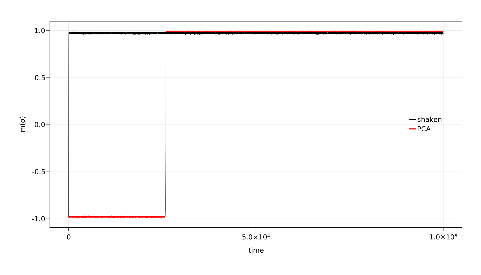
A similar behavior has been highlighted in [12, 13] where a comparison between the symmetric PCA and an irreversible PCA with totally asymmetric interaction has been performed in the case λ=0\lambda=0. In the case of null magnetic field, if the value of the inverse temperature β\beta is large but finite, the system exhibits, both in the case of PCA dynamics and shaken dynamics, a (positive or negative) spontaneous magnetization. On short time scales the system stays in one “phase” (e.g. it is negatively magnetized) whereas, on longer time scales, it tunnels rapidly towards the other phase. However, since the value of the spontaneous magnetization is neither exactly −1-1 or +1+1, choosing the right parameters to compare the two dynamics, as far as tunneling time is concerned, may be a somewhat delicate matter. To make a fair comparison of the tunneling times we tuned the parameters of the PCA and the shaken dynamics so to have similar values for the (average) spontaneous magnetization. The results of the experiment are summarized in Figure 5 where the average magnetization over time is represented for both dynamics. It is evident that, also in this case, the shaken dynamics has considerably more mobility than the PCA. As far as the tunneling behavior is concerned, the shaken dynamics retains, essentially, the same features of the irreversible PCA considered in [13]. However, it is to remark that, in the case of the shaken dynamics, reversibility allows to manage the invariant measure more easily.
Refer to caption
(a) β=1.3,q=0.1,λ=0.15\beta=1.3,q=0.1,\lambda=0.15
(b) β=2.3,q=0.1,λ=0.15\beta=2.3,q=0.1,\lambda=0.15
(c) β=3.3,q=0.1,λ=0.15\beta=3.3,q=0.1,\lambda=0.15
(d) β=4.0,q=0.1,λ=0.15\beta=4.0,q=0.1,\lambda=0.15
Figure 4: Comparison of the magnetization over time for PCA and shaken dynamics for growing values of the inverse tempeature β\beta.
Figure 5: Comparison of the evolution of the magnetization for a spin system evolving according to a shaken dynamics (black) and according to a symmetric PCA (red). The values of the parameters are such that both dynamics exhibit the same spontaneous magnetization and are consistent with those of [13].

4 Geometrical discussion

In the shaken dynamics the idea of alternate dynamics is combined with that of the doubling Hamiltonian. Indeed considering only part of the interaction (for instance down-left first and then up-right in the case of Λ∈ℤ2\Lambda\in\mathbb{Z}^{2} presented at the beginning of the Section) and introducing the inertial parameter of self interaction qq it is possible to interpolate between different lattice geometries induced by the doubling graph as already discussed in [1].

Indeed the alternate dynamics on the hexagonal lattice makes possible to interpolate between the square (q→∞q\to\infty) and the 1-dimensional lattice (q→0q\to 0). The interpolation between lattices induced by the shaken dynamics may be applied in general, and in the case of planar graphs the results concerning the critical behavior contained in [1] can be extended, using [3].

Consider for instance the Ising model on the triangular lattice. On this lattice we divide the 6 nearest neighbors of each vertex xx into two sets, e.g. ℓ⁡(x)\ell(x) left and r⁡(x)r(x) right nearest neighbors of xx, and define a shaken dynamics with self interaction qq. Hence the doubled Hamiltonian is

H△(σ,τ)=−∑x[∑y∈ℓ⁡(x)(Jσyτx)+qσxτx]=−∑x[∑y∈r⁡(x)(Jτyσx)+qσxτx]H^{\triangle}(\sigma,\tau)=-\sum_{x}\Big[\sum_{y\in\ell(x)}\big(J\sigma_{y}\tau_{x}\big)+q\sigma_{x}\tau_{x}\Big]=-\sum_{x}\Big[\sum_{y\in r(x)}\big(J\tau_{y}\sigma_{x}\big)+q\sigma_{x}\tau_{x}\Big]

The corresponding alternate dynamics turns out to be defined on the square lattice (see Fig. 6) with invariant measure the Gibbs one. In particular the square lattice is regular when we set J=qJ=q. In this case the parameter qq can be used to move through different geometries. The triangular lattice (q→∞q\to\infty) and the hexagonal lattice (q=0q=0) can be derived from the original square lattice just tuning the value of qq. A more precise statement of this interpolation is given by the following

Theorem 4.1

For the shaken dynamics on the triangular lattice the critical equation relating the parameters JJ and qq is given by

1+tanh3⁡(J)​tanh⁡(q)=3​tanh⁡(J)​tanh⁡(q)+3​tanh2⁡(J)\displaystyle 1+\tanh^{3}(J)\tanh(q)=3\tanh(J)\tanh(q)+3\tanh^{2}(J) (26)

In the case q=Jq=J we obtain the Onsager critical temperature for the square lattice, for q=0q=0 we obtain the critical temperature for the hexagonal lattice and in the limit q→∞q\to\infty we obtain the critical temperature for the triangular lattice.

Figure 6: Interaction in the pair Hamiltonian for the shaken dynamics on the triangular lattice. Each spin of configuration σ\sigma (living on the solid lattice) interacts with the spin at the same location and the three spins on its left in τ\tau (living on the dashed lattice). The darker lines show that the pair interaction lives on a rectangular lattice. For q=Jq=J this lattice becomes the square one. As q→∞q\to\infty the square lattice collapses onto the triangular lattice. If q=0q=0 the interaction graph becomes the homogeneous hexagonal lattice.

5 The generalized shaken dynamics

We can generalize the construction of the shaken dynamics. Starting from a symmetric interaction 𝒥{\cal J} defining the Hamiltonian H⁡(σ)H(\sigma), as in (2), we can define an arbitrary decomposition of the interaction matrix 𝒥{\cal J} in a sum of two matrices with non negative entries

𝒥=𝒥o+𝒥oT.{\cal J}={\cal J}^{o}+{{\cal J}^{o}}^{T}. (27)

This means that every non oriented edge {x,y}\{x,y\} with weight Jx​yJ_{xy} is decomposed in a pair of oriented edges (x,y)(x,y) and (y,x)(y,x) with weight respectively 𝒥x​yo{\cal J}^{o}_{xy} and 𝒥y​xo{\cal J}^{o}_{yx}. Call EoE^{o} the set of all these oriented edges and apply the construction presented in Section 2 to construct the doubling graph by using this set EoE^{o} of oriented edges.

We proceed as before defining the doubling Hamiltonian

H⁡(σ(1),σ(2))=−⟨σ(1),𝒥o​σ(2)⟩−q⁡⟨σ(1),σ(2)⟩−⟨λ,σ(1)⟩−⟨λ,σ(2)⟩=−⟨𝒥oT​σ(1),σ(2)⟩−q⁡⟨σ(1),σ(2)⟩−⟨λ,σ(1)⟩−⟨λ,σ(2)⟩.\displaystyle\begin{aligned} H(\sigma^{(1)},\sigma^{(2)})&=-\langle\sigma^{(1)},{{\cal J}^{o}}\sigma^{(2)}\rangle-q\langle\sigma^{(1)},\sigma^{(2)}\rangle-\langle\lambda,\sigma^{(1)}\rangle-\langle\lambda,\sigma^{(2)}\rangle\\ &=-\langle{{\cal J}^{o}}^{T}\sigma^{(1)},\sigma^{(2)}\rangle-q\langle\sigma^{(1)},\sigma^{(2)}\rangle-\langle\lambda,\sigma^{(1)}\rangle-\langle\lambda,\sigma^{(2)}\rangle.\end{aligned} (28)

In the case σ(1)=σ(2)=σ\sigma^{(1)}=\sigma^{(2)}=\sigma by equation (27) we have again H⁡(σ,σ)=H⁡(σ)−q​|V|H(\sigma,\sigma)=H(\sigma)-q|V|.

The corresponding alternate dynamics on the state space 𝒳V{\cal X}_{V} is defined with two subsequent updating as follows:

P1→2​(σ,σ′):=e−β​H​(σ,σ′)Z→σ,P2→1​(σ′,τ):=e−β​H​(τ,σ′)Z←σ′P^{1\to 2}(\sigma,\sigma^{\prime}):=\frac{e^{-\beta H(\sigma,\sigma^{\prime})}}{\overrightarrow{Z}_{\sigma}},\qquad P^{2\to 1}(\sigma^{\prime},\tau):=\frac{e^{-\beta H(\tau,\sigma^{\prime})}}{\overleftarrow{Z}_{\sigma^{\prime}}} (29)

and

Ps​h​(σ,τ)=∑σ′∈𝒳VP1→2​(σ,σ′)​P2→1​(σ′,τ)=∑σ′∈𝒳Ve−β​H​(σ,σ′)Z→σ​e−β​H​(τ,σ′)Z←σ′P^{sh}(\sigma,\tau)=\sum_{\sigma^{\prime}\in{\cal X}_{V}}P^{1\to 2}(\sigma,\sigma^{\prime})P^{2\to 1}(\sigma^{\prime},\tau)=\sum_{\sigma^{\prime}\in{\cal X}_{V}}\frac{e^{-\beta H(\sigma,\sigma^{\prime})}}{\overrightarrow{Z}_{\sigma}}\frac{e^{-\beta H(\tau,\sigma^{\prime})}}{\overleftarrow{Z}_{\sigma^{\prime}}} (30)

The results obtained in Theorem 2.3 can be immediately extended to this more general case.

The choice of the shaken dynamics discussed in Section 2 is a particular case of generalized shaken dynamics in which 𝒥x​yo​𝒥y​xo=0{\cal J}^{o}_{xy}{\cal J}^{o}_{yx}=0 for any pair x,yx,y. In the general case the geometrical discussion of the doubling graph of interaction is much more complicated. Also the interpolation between different geometries obtained for different values of the parameter qq, as discussed in Section 3, is more involved in this generalized case.

Refer to caption
Figure 7: The construction of the doubling graph in the case of the generalized shaken dynamics.

Another particular choice in this class of generalized shaken dynamics is 𝒥o=12​𝒥{\cal J}^{o}=\frac{1}{2}{\cal J} corresponding to the PCA discussed in [6].

6 Application to optimization problems

The shaken dynamics on a general graph, and its generalization, gets the possibility to look for the minimum of a general Hamiltonian H⁡(σ)H(\sigma) defined on {−1,+1}V\{-1,+1\}^{V} by means of a parallel dynamics, by using the following result that could be considered a corollary of Theorem 2.3. In combinatorial optimization this can be used as a parallel approach to the Quadratic Unconstrained Binary Optimization (QUBO) i.e., the problem of minimizing a quadratic polynomial of binary variables (see [10] for a survey).

Theorem 6.1

Consider a Hamiltonian H⁡(σ)H(\sigma) of the form given in (28) on {−1,+1}V\{-1,+1\}^{V}, for any doubling Hamiltonian H⁡(σ,τ)H(\sigma,\tau) defined in (3), corresponding to a bipartite graph Gb=(Vb,Eb)G^{b}=(V^{b},E^{b}).

  1. (1)

    If

    q>maxx∈V{∑y:{x,y}∈Eb|Jx​y|+|λx|}\displaystyle q>\max_{x\in V}\Big\{\sum_{y:\{x,y\}\in E^{b}}|J_{xy}|+|\lambda_{x}|\Big\} (31)

    then the alternate dynamics defined with H⁡(σ,τ)H(\sigma,\tau) is a parallel algorithm to find configurations σ\sigma minimizing H⁡(σ)H(\sigma).

  2. (2)

    For any positive qq the alternate dynamics defined with H⁡(σ,τ)H(\sigma,\tau) is a parallel algorithm to find a lower bound for minσ⁡H⁡(σ)\min_{\sigma}H(\sigma).

To assess the effectiveness of the strategy presented in Theorem 6.1, we put forward some preliminary tests on a simplified version of the Edwards-Anderson model where the weight of the edges connecting neighboring sites is set to J=+1J=+1 with probability 12\frac{1}{2} and J=−1J=-1 with probability 12\frac{1}{2} and where the external field is zero. In this case, setting q>2q>2 is sufficient to satisfy the hypotheses of the corollary. We compared the results with those obtained with a single spin flip heat bath dynamics and considered “grids” with side length 128 and 256. With this setting, the heuristic minima that we obtained with the shaken dynamics are essentially equivalent to those obtained with the single spin flip dynamics. However the speed up with respect to the single spin flip dynamics was significant. To be as fair as possible in this comparison, we renormalized the time of the single spin flip dynamics with the number of vertices in the graph so to have the same number of “attempted spin flips”. We observed a speed-up of about 10 times when considering, for both algorithms, a CPU implementation and up to 200 times when comparing the CPU implementation of the single spin flip dynamics with a GPU implementation of the shaken dynamics. These findings are in agreement with Theorem 3.2.

7 Proofs of the results

7.1 Proof of Theorem 2.3

We have immediately the detailed balance condition w.r.t. the measure π⁡(σ)\pi(\sigma) indeed

∑σ′∈𝒳Ve−β⁡(H⁡(σ,σ′)+H⁡(τ,σ′))Z←σ′=Z→σ​Ps​h​(σ,τ)=Z→τ​Ps​h​(τ,σ)=∑σ′∈𝒳Ve−β⁡(H⁡(τ,σ′)+H⁡(σ,σ′))Z←σ′\sum_{\sigma^{\prime}\in{\cal X}_{V}}\frac{e^{-\beta(H(\sigma,\sigma^{\prime})+H(\tau,\sigma^{\prime}))}}{\overleftarrow{Z}_{\sigma^{\prime}}}=\overrightarrow{Z}_{\sigma}P^{sh}(\sigma,\tau)=\overrightarrow{Z}_{\tau}P^{sh}(\tau,\sigma)=\sum_{\sigma^{\prime}\in{\cal X}_{V}}\frac{e^{-\beta(H(\tau,\sigma^{\prime})+H(\sigma,\sigma^{\prime}))}}{\overleftarrow{Z}_{\sigma^{\prime}}} (32)

It is straightforward to prove that πb​(σ(1),σ(2)){\pi^{b}}(\sigma^{(1)},\sigma^{(2)}) is the stationary measure of Pa​l​tP^{alt}

∑σ(1),σ(2)πb​(σ(1),σ(2))​Pa​l​t​(𝝈,𝝉)=∑σ(1),σ(2)e−β​H​(σ(1),σ(2))Z​e−β​H​(σ(1),τ(2))Z→σ(1)​e−β​H​(τ(1),τ(2))Z←τ(2)=e−β​H​(τ(1),τ(2))Z=πb​(τ(1),τ(2))\displaystyle\begin{aligned} \sum_{\sigma^{(1)},\sigma^{(2)}}{{\pi^{b}}}(\sigma^{(1)},\sigma^{(2)})P^{alt}(\hbox{{\boldmath$\sigma$},{\boldmath$\tau$}})&=\sum_{\sigma^{(1)},\sigma^{(2)}}\frac{e^{-\beta H(\sigma^{(1)},\sigma^{(2)})}}{Z}\frac{e^{-\beta H(\sigma^{(1)},\tau^{(2)})}}{\overrightarrow{Z}_{\sigma^{(1)}}}\frac{e^{-\beta H(\tau^{(1)},\tau^{(2)})}}{\overleftarrow{Z}_{\tau^{(2)}}}\\ &=\frac{e^{-\beta H(\tau^{(1)},\tau^{(2)})}}{Z}={\pi^{b}}(\tau^{(1)},\tau^{(2)})\end{aligned} (33)

□\hfill{\square\hfill}

Note that, in general

πb​(σ(1),σ(2))​Pa​l​t​(𝝈,𝝉)≠πb​(τ(1),τ(2))​Pa​l​t​(𝝉,𝝈).{{\pi^{b}}}(\sigma^{(1)},\sigma^{(2)})P^{alt}(\hbox{{\boldmath$\sigma$},{\boldmath$\tau$}})\not={{\pi^{b}}}(\tau^{(1)},\tau^{(2)})P^{alt}(\hbox{{\boldmath$\tau$},{\boldmath$\sigma$}}).

For instance consider the bipartite graphs Kn,nK_{n,n} with equal weights on all edges and where, for all ii, (σi(1),σi(2))=(+1,+1)(\sigma_{i}^{(1)},\sigma_{i}^{(2)})=(+1,+1) and (τi(1),τi(2))=(+1,−1)(\tau_{i}^{(1)},\tau_{i}^{(2)})=(+1,-1).

7.2 Proof of Theorem 3.1

To prove Theorem 3.1 it is possible to argue as in the proof of Theorem 1.2 in [16].

In our notation πΛ\pi_{\Lambda} and πΛG\pi_{\Lambda}^{G} have the role, respectively, of πP​C​A\pi_{PCA} and πG\pi_{G} used in [16]. Further let gx​(σ):=J⁡(σx↓+σx←)g_{x}(\sigma):=J(\sigma_{x^{\downarrow}}+\sigma_{x^{\leftarrow}}) be the analogue of hi​(σ)h_{i}(\sigma) in [16]. Here we assume λ<0\lambda<0. The case λ>0\lambda>0 can be treated likewise.

Recalling that δ=e−2​β​q\delta=e^{-2\beta q}, it is possible to write Z→σ\overrightarrow{Z}_{\sigma} in the following way:

Z→σ=∑τe−β​H​(σ,τ)=∑τe−β​H​(σ,σ)​e−β⁡[H⁡(σ,τ)−H⁡(σ,σ)]=eβ​q​|Λ|e−β​H​(σ)∑τeβ∑x:σx≠τx−2gx(σ)σx−2q−2λσx=eβ​q​|Λ|​e−β​H​(σ)​∑I⊂Λδ|I|​∏x∈Ie−β⁡(2​gx​(σ)​σx+2​λ​σx)=eβ​q​|Λ|​e−β​H​(σ)​∏x∈Λ(1+δ​e−β⁡(2​gx​(σ)​σx+2​λ​σx))\displaystyle\begin{aligned} \overrightarrow{Z}_{\sigma}&=\sum_{\tau}e^{-\beta H(\sigma,\tau)}=\sum_{\tau}e^{-\beta H(\sigma,\sigma)}e^{-\beta[H(\sigma,\tau)-H(\sigma,\sigma)]}\\ &=e^{\beta q|\Lambda|}e^{-\beta H(\sigma)}\sum_{\tau}e^{\beta\sum_{x:\sigma_{x}\neq\tau_{x}}-2g_{x}(\sigma)\sigma_{x}-2q-2\lambda\sigma_{x}}\\ &=e^{\beta q|\Lambda|}e^{-\beta H(\sigma)}\sum_{I\subset\Lambda}\delta^{|I|}\prod_{x\in I}e^{-\beta(2g_{x}(\sigma)\sigma_{x}+2\lambda\sigma_{x})}\\ &=e^{\beta q|\Lambda|}e^{-\beta H(\sigma)}\prod_{x\in\Lambda}(1+\delta e^{-\beta(2g_{x}(\sigma)\sigma_{x}+2\lambda\sigma_{x})})\end{aligned} (34)

where the sum over τ\tau has been rewritten as the sum over all subsets I⊂ΛI\subset\Lambda such that τx=−σx\tau_{x}=-\sigma_{x} if x∈Ix\in I and τx=σx\tau_{x}=\sigma_{x} otherwise. The factor eβ​q​|Λ|e^{\beta q|\Lambda|} does not depend on σ\sigma and cancels out in the ratio Z→σZ\frac{\overrightarrow{Z}_{\sigma}}{Z}.

Call f⁡(σ):=∏x∈Λ(1+δ​e−β⁡(2​gx​(σ)​σx+2​λ​σx))f(\sigma):=\prod_{x\in\Lambda}(1+\delta e^{-\beta(2g_{x}(\sigma)\sigma_{x}+2\lambda\sigma_{x})}),   w⁡(σ):=e−β​H​(σ)​f​(σ)=wG​(σ)​f​(σ)w(\sigma):=e^{-\beta H(\sigma)}f(\sigma)=w^{G}(\sigma)f(\sigma). Then, by (34), it follows

πΛ​(σ)\displaystyle\pi_{\Lambda}(\sigma) =w⁡(σ)∑τw⁡(τ)=wG​(σ)​f​(σ)∑τwG​(τ)​f​(τ)=wG​(σ)ZG​f​(σ)∑τwG​(τ)ZG​f​(τ)=πΛG​(σ)​f​(σ)πΛG​(f)\displaystyle=\frac{w(\sigma)}{\sum_{\tau}w(\tau)}=\frac{w^{G}(\sigma)f(\sigma)}{\sum_{\tau}w^{G}(\tau)f(\tau)}=\frac{\frac{w^{G}(\sigma)}{Z^{G}}f(\sigma)}{\sum_{\tau}\frac{w^{G}(\tau)}{Z^{G}}f(\tau)}=\frac{\pi_{\Lambda}^{G}(\sigma)f(\sigma)}{\pi_{\Lambda}^{G}(f)}

with πΛG​(f)=∑σπΛG​(σ)​f​(σ)\pi_{\Lambda}^{G}(f)=\sum_{\sigma}\pi_{\Lambda}^{G}(\sigma)f(\sigma).

As in [16], using Jensen’s inequality the total variation distance between πΛ\pi_{\Lambda} and πΛG\pi_{\Lambda}^{G} can be bounded as

‖πΛ−πΛG‖T​V≤πΛG​(f2)(πΛG​(f))2−1=:(Δ⁡(δ)).\displaystyle\|\pi_{\Lambda}-\pi_{\Lambda}^{G}\|_{TV}\leq\sqrt{\frac{\pi_{\Lambda}^{G}(f^{2})}{(\pi_{\Lambda}^{G}(f))^{2}}-1}=:\sqrt{(\Delta(\delta))}.

To prove the theorem, it will be shown that Δ⁡(δ)=O⁡(δ2​|Λ|)\Delta(\delta)=O(\delta^{2}|\Lambda|).

By writing Δ⁡(δ)=elog⁡(πΛG​(f2))−2​log⁡(πΛG​(f))−1,\Delta(\delta)=e^{\log(\pi_{\Lambda}^{G}(f^{2}))-2\log(\pi_{\Lambda}^{G}(f))}-1, the claim follows by showing that the argument of the exponential divided by |Λ||\Lambda| is analytic in δ\delta and that the first order term of its expansion in δ\delta cancels out.

In other words the claim follows thanks to the following lemma.

Lemma 7.1

There exists JcJ_{c} such that, for all J>JcJ>J_{c}

  1. 1.

    log⁡(πΛG​(f2))|Λ|\frac{\log(\pi_{\Lambda}^{G}(f^{2}))}{|\Lambda|} and log⁡(πΛG​(f))|Λ|\frac{\log(\pi_{\Lambda}^{G}(f))}{|\Lambda|} are analytic in δ\delta for |δ|<δJ|\delta|<\delta_{J}

  2. 2.

    log⁡(πΛG​(f2))|Λ|−2​log⁡(πΛG​(f))|Λ|=O⁡(δ2)\frac{\log(\pi_{\Lambda}^{G}(f^{2}))}{|\Lambda|}-2\frac{\log(\pi_{\Lambda}^{G}(f))}{|\Lambda|}=O(\delta^{2})

Proof: The analyticity of log⁡(πΛG​(f2))|Λ|\frac{\log(\pi_{\Lambda}^{G}(f^{2}))}{|\Lambda|} and log⁡(πΛG​(f))|Λ|\frac{\log(\pi_{\Lambda}^{G}(f))}{|\Lambda|} is proven by showing that these quantities can be written as partition functions of an abstract polymer gas. The analyticity is obtained using standard cluster expansion.

To carry over this task, we will rewrite πΛG​(fk)\pi_{\Lambda}^{G}(f^{k}) in terms of standard Peierls contours. Divide the sites in Λ\Lambda according to the value of the spins and number of edges of the Peierls contour left and below the site in the following way:

  • Λ​−⁣−−\Lambda\negthinspace{\genfrac{}{}{0.0pt}{2}{--}{\phantom{-}-}}: {x∈Λ:σx=−1∧(σx←=−1,σx↓=−1)}\{x\in\Lambda:\sigma_{x}=-1\land(\sigma_{x^{\leftarrow}}=-1,\sigma_{x^{\downarrow}}=-1)\};

  • Λ​+⁣−−\Lambda\negthinspace{\genfrac{}{}{0.0pt}{2}{+-}{\phantom{-}-}}: {x∈Λ:σx=−1∧((σx←=+1,σx↓=−1)∨(σx←=−1,σx↓=+1))}\{x\in\Lambda:\sigma_{x}=-1\land((\sigma_{x^{\leftarrow}}=+1,\sigma_{x^{\downarrow}}=-1)\lor(\sigma_{x^{\leftarrow}}=-1,\sigma_{x^{\downarrow}}=+1))\};

  • Λ​+⁣−+\Lambda\negthinspace{\genfrac{}{}{0.0pt}{2}{+-}{\phantom{-}+}}: {x∈Λ:σx=−1∧σx←=+1,σx↓=+1}\{x\in\Lambda:\sigma_{x}=-1\land\sigma_{x^{\leftarrow}}=+1,\sigma_{x^{\downarrow}}=+1\};

  • Λ​+⁣++\Lambda\negthinspace{\genfrac{}{}{0.0pt}{2}{++}{\phantom{-}+}}: {x∈Λ:σx=+1∧(σx←=+1,σx↓=+1)}\{x\in\Lambda:\sigma_{x}=+1\land(\sigma_{x^{\leftarrow}}=+1,\sigma_{x^{\downarrow}}=+1)\};

  • Λ​−⁣++\Lambda\negthinspace{\genfrac{}{}{0.0pt}{2}{-+}{\phantom{-}+}}: {x∈Λ:σx=+1∧((σx←=+1,σx↓=−1)∨(σx←=−1,σx↓=+1))}\{x\in\Lambda:\sigma_{x}=+1\land((\sigma_{x^{\leftarrow}}=+1,\sigma_{x^{\downarrow}}=-1)\lor(\sigma_{x^{\leftarrow}}=-1,\sigma_{x^{\downarrow}}=+1))\};

  • Λ​−⁣+−\Lambda\negthinspace{\genfrac{}{}{0.0pt}{2}{-+}{\phantom{-}-}}: {x∈Λ:σx=+1∧(σx←=−1,σx↓=−1)}\{x\in\Lambda:\sigma_{x}=+1\land(\sigma_{x^{\leftarrow}}=-1,\sigma_{x^{\downarrow}}=-1)\};

With this notation, f⁡(σ)f(\sigma) can be written as

f⁡(σ)=[1+δ​eβ⁡(−4​J+2​λ)]|Λ|​∏x∈Λ​+⁣−−(1+δ​e+2​β​λ)[1+δ​eβ⁡(−4​J+2​λ)]​∏x∈Λ​+⁣−+[1+δ​eβ⁡(4​J+2​λ)][1+δ​eβ⁡(−4​J+2​λ)]∏x∈Λ​+⁣++[1+δ​eβ⁡(−4​J−2​λ)][1+δ​eβ⁡(−4​J+2​λ)]​∏x∈Λ​−⁣++(1+δ​e−2​β​λ)[1+δ​eβ⁡(−4​J+2​λ)]​∏x∈Λ​−⁣+−[1+δ​eβ⁡(4​J−2​λ)][1+δ​eβ⁡(−4​J+2​λ)]=[1+δ​eβ⁡(−4​J+2​λ)]|Λ|​ξ~​(σ,λ)\displaystyle\begin{aligned} f(\sigma)&=[1+\delta e^{\beta(-4J+2\lambda)}]^{|\Lambda|}\prod_{x\in\Lambda\negthinspace{\genfrac{}{}{0.0pt}{2}{+-}{\phantom{-}-}}}\frac{(1+\delta e^{+2\beta\lambda})}{[1+\delta e^{\beta(-4J+2\lambda)}]}\prod_{x\in\Lambda\negthinspace{\genfrac{}{}{0.0pt}{2}{+-}{\phantom{-}+}}}\frac{[1+\delta e^{\beta(4J+2\lambda)}]}{[1+\delta e^{\beta(-4J+2\lambda)}]}\\ &\prod_{x\in\Lambda\negthinspace{\genfrac{}{}{0.0pt}{2}{++}{\phantom{-}+}}}\frac{[1+\delta e^{\beta(-4J-2\lambda)}]}{[1+\delta e^{\beta(-4J+2\lambda)}]}\prod_{x\in\Lambda\negthinspace{\genfrac{}{}{0.0pt}{2}{-+}{\phantom{-}+}}}\frac{(1+\delta e^{-2\beta\lambda})}{[1+\delta e^{\beta(-4J+2\lambda)}]}\prod_{x\in\Lambda\negthinspace{\genfrac{}{}{0.0pt}{2}{-+}{\phantom{-}-}}}\frac{[1+\delta e^{\beta(4J-2\lambda)}]}{[1+\delta e^{\beta(-4J+2\lambda)}]}\\ &=[1+\delta e^{\beta(-4J+2\lambda)}]^{|\Lambda|}\tilde{\xi}(\sigma,\lambda)\end{aligned} (35)

with

ξ~​(σ,λ)=[(1+δ​e+2​β​λ)[1+δ​eβ⁡(−4​J+2​λ)]]|Λ​+⁣−−|×[[1+δ​eβ⁡(4​J+2​λ)][1+δ​eβ⁡(−4​J+2​λ)]]|Λ​+⁣−+|×[[1+δ​eβ⁡(−4​J−2​λ)][1+δ​eβ⁡(−4​J+2​λ)]]|Λ​+⁣++|×[(1+δ​e−2​β​λ)[1+δ​eβ⁡(−4​J+2​λ)]]|Λ​−⁣++|×[[1+δ​eβ⁡(4​J−2​λ)][1+δ​eβ⁡(−4​J+2​λ)]]|Λ​−⁣+−|\displaystyle\begin{aligned} \tilde{\xi}(\sigma,\lambda)=&\left[\frac{(1+\delta e^{+2\beta\lambda})}{[1+\delta e^{\beta(-4J+2\lambda)}]}\right]^{\left|\Lambda\negthinspace{\genfrac{}{}{0.0pt}{2}{+-}{\phantom{-}-}}\right|}\,\times\,\left[\frac{[1+\delta e^{\beta(4J+2\lambda)}]}{[1+\delta e^{\beta(-4J+2\lambda)}]}\right]^{\left|\Lambda\negthinspace{\genfrac{}{}{0.0pt}{2}{+-}{\phantom{-}+}}\right|}\,\times\,\\ &\left[\frac{[1+\delta e^{\beta(-4J-2\lambda)}]}{[1+\delta e^{\beta(-4J+2\lambda)}]}\right]^{\left|\Lambda\negthinspace{\genfrac{}{}{0.0pt}{2}{++}{\phantom{-}+}}\right|}\,\times\,\left[\frac{(1+\delta e^{-2\beta\lambda})}{[1+\delta e^{\beta(-4J+2\lambda)}]}\right]^{\left|\Lambda\negthinspace{\genfrac{}{}{0.0pt}{2}{-+}{\phantom{-}+}}\right|}\,\times\,\\ &\left[\frac{[1+\delta e^{\beta(4J-2\lambda)}]}{[1+\delta e^{\beta(-4J+2\lambda)}]}\right]^{\left|\Lambda\negthinspace{\genfrac{}{}{0.0pt}{2}{-+}{\phantom{-}-}}\right|}\end{aligned} (36)

For a given a configuration σ∈𝒳Λ\sigma\in{\cal X}_{\Lambda}, we denote by γ⁡(σ)\gamma(\sigma) its Peierls contour in the dual ℬΛ∗=∪(x,y)∈ℬΛ(x,y)∗{\cal B}_{\Lambda}^{*}=\cup_{(x,y)\in{\cal B}_{\Lambda}}(x,y)^{*}

γ⁡(σ):={(x,y)∗∈ℬΛ∗:σx​σy=−1}\gamma(\sigma):=\{(x,y)^{*}\in{\cal B}_{\Lambda}^{*}:\;\sigma_{x}\sigma_{y}=-1\} (37)

Noting that e−β​H​(σ)=e(2​J−2​λ)​β​|Λ|​e−2​β​J​|γ⁡(σ)​|+4​β​λ|​V+​(σ)|e^{-\beta H(\sigma)}=e^{(2J-2\lambda)\beta|\Lambda|}e^{-2\beta J|\gamma(\sigma)|+4\beta\lambda|V_{+}(\sigma)|}, with |V+(σ)|=∑x∈Λ1{σx=+1}|V_{+}(\sigma)|=\sum_{x\in\Lambda}1_{\{\sigma_{x}=+1\}} is the number of plus spins in Λ\Lambda of configuration σ\sigma, we have

πΛG​(fk)=1ZG​e(2​J−2​λ)​β​|Λ|​[1+δ​eβ⁡(−4​J+2​λ)]k​|Λ|​∑σ[e−2​β​J​|γ⁡(σ)​|+4​β​λ|​V+​(σ)|​ξ~​(σ,λ)k]\displaystyle\pi_{\Lambda}^{G}(f^{k})=\frac{1}{Z^{G}}e^{(2J-2\lambda)\beta|\Lambda|}[1+\delta e^{\beta(-4J+2\lambda)}]^{k|\Lambda|}\sum_{\sigma}\left[e^{-2\beta J|\gamma(\sigma)|+4\beta\lambda|V_{+}(\sigma)|}\tilde{\xi}(\sigma,\lambda)^{k}\right] (38)

Setting

ξ⁡(σ,λ)=[(1+δ​e+2​β​λ)[1+δ​eβ⁡(−4​J+2​λ)]]|Λ​+⁣−−|×[[1+δ​eβ⁡(4​J+2​λ)]×[1+δeβ⁡(−4​J+2​λ)]]|Λ​+⁣−+|×[e+2​β​λ​[1+δ​eβ⁡(−4​J−2​λ)][1+δ​eβ⁡(−4​J+2​λ)]]|Λ​+⁣++|×[e+2​β​λ​(1+δ​e−2​β​λ)[1+δ​eβ⁡(−4​J+2​λ)]]|Λ​−⁣++|×[e+2​β​λ​[1+δ​eβ⁡(4​J−2​λ)][1+δ​eβ⁡(−4​J+2​λ)]]|Λ​−⁣+−|\displaystyle\begin{aligned} \xi(\sigma,\lambda)=&\left[\frac{(1+\delta e^{+2\beta\lambda})}{[1+\delta e^{\beta(-4J+2\lambda)}]}\right]^{\left|\Lambda\negthinspace{\genfrac{}{}{0.0pt}{2}{+-}{\phantom{-}-}}\right|}\,\times\,\left[\frac{[1+\delta e^{\beta(4J+2\lambda)}]}{\,}\times\,{[1+\delta e^{\beta(-4J+2\lambda)}]}\right]^{\left|\Lambda\negthinspace{\genfrac{}{}{0.0pt}{2}{+-}{\phantom{-}+}}\right|}\,\times\,\\ &\left[\frac{e^{+2\beta\lambda}[1+\delta e^{\beta(-4J-2\lambda)}]}{[1+\delta e^{\beta(-4J+2\lambda)}]}\right]^{\left|\Lambda\negthinspace{\genfrac{}{}{0.0pt}{2}{++}{\phantom{-}+}}\right|}\,\times\,\left[\frac{e^{+2\beta\lambda}(1+\delta e^{-2\beta\lambda})}{[1+\delta e^{\beta(-4J+2\lambda)}]}\right]^{\left|\Lambda\negthinspace{\genfrac{}{}{0.0pt}{2}{-+}{\phantom{-}+}}\right|}\,\times\,\\ &\left[\frac{e^{+2\beta\lambda}[1+\delta e^{\beta(4J-2\lambda)}]}{[1+\delta e^{\beta(-4J+2\lambda)}]}\right]^{\left|\Lambda\negthinspace{\genfrac{}{}{0.0pt}{2}{-+}{\phantom{-}-}}\right|}\end{aligned} (39)

allows us to write, for k∈{1,2}k\in\{1,2\},

∑σ[e−2​β​J​|γ⁡(σ)​|+4​β​λ|​V+​(σ)|​ξ~​(σ,λ)k]=∑σ[e−2​β​J​|γ⁡(σ)|​(e+2​β​λ​|V+​(σ)|)2−k​ξ​(σ,λ)k]\displaystyle\sum_{\sigma}\left[e^{-2\beta J|\gamma(\sigma)|+4\beta\lambda|V_{+}(\sigma)|}\tilde{\xi}(\sigma,\lambda)^{k}\right]=\sum_{\sigma}\left[e^{-2\beta J|\gamma(\sigma)|}\left(e^{+{2\beta\lambda|V_{+}(\sigma)|}}\right)^{2-k}\xi(\sigma,\lambda)^{k}\right] (40)

A straightforward computation yields ξ​(σ,λ)k≤ξ​(σ,0)k\xi(\sigma,\lambda)^{k}\leq\xi(\sigma,0)^{k} and then

∑σ[e−2​β​J​|γ⁡(σ)|​(e+2​β​λ​|V+​(σ)|)2−k​ξ​(σ,λ)k]\displaystyle\sum_{\sigma}\left[e^{-2\beta J|\gamma(\sigma)|}\left(e^{+{2\beta\lambda|V_{+}(\sigma)|}}\right)^{2-k}\xi(\sigma,\lambda)^{k}\right] d≤∑σe−2​β​J​|γ⁡(σ)|​ξ​(σ,0)k\displaystyle d\leq\sum_{\sigma}e^{-2\beta J|\gamma(\sigma)|}\xi(\sigma,0)^{k} (41)
=2​∑γe−2​β​J​|γ|​ξ​(γ,0)k\displaystyle=2\sum_{\gamma}e^{-2\beta J|\gamma|}\xi(\gamma,0)^{k}

where ξ​(γ,0)k\xi(\gamma,0)^{k} coincides with ξkI​(Γ)\xi^{I}_{k}(\Gamma) in the proof of Lemma 2.3 in [16], with |Λ​+⁣−−|+|Λ​−⁣++|=|l1​(Γ)|\left|\Lambda\negthinspace{\genfrac{}{}{0.0pt}{2}{+-}{\phantom{-}-}}\right|+\left|\Lambda\negthinspace{\genfrac{}{}{0.0pt}{2}{-+}{\phantom{-}+}}\right|=|l_{1}(\Gamma)| and |Λ​+⁣−+|+|Λ​−⁣+−|=|l2​(Γ)|\left|\Lambda\negthinspace{\genfrac{}{}{0.0pt}{2}{+-}{\phantom{-}+}}\right|+\left|\Lambda\negthinspace{\genfrac{}{}{0.0pt}{2}{-+}{\phantom{-}-}}\right|=|l_{2}(\Gamma)|.

This implies that the proof can be concluded following the same steps as in [16]. □\square

7.3 Proof of Theorem  3.3

Starting from −𝟙-\mathbb{1} the first spin flip is a move against the drift having a probability e−2​β​|hxS​h​(−𝟙)|=e−2​β​(2​J+q−λ)e^{-2\beta|h^{Sh}_{x}(-\mathbb{1})|}=e^{-2\beta(2J+q-\lambda)} for some x∈Λx\in\Lambda. Different exits from −𝟙-\mathbb{1}, with more than a single spin flip, have a probability exponentially smaller than this. Hence, denoting for simplicity a configuration with the set of its plus spins, we have Xτ−𝟙cS​h={x}X^{Sh}_{\tau_{-\mathbb{1}^{c}}}=\{x\} and therefore

limβ→∞P−𝟙S​h({τ−𝟙c<Tδ/2}∩{Xτ−𝟙cS​h={x} for some x∈Λ})=1.\lim_{\beta\to\infty}P^{Sh}_{-\mathbb{1}}\Big(\{\tau_{-\mathbb{1}^{c}}<T_{\delta/2}\}\cap\{X^{Sh}_{\tau_{-\mathbb{1}^{c}}}=\{x\}\,\hbox{ for some }x\in\Lambda\}\Big)=1.

Starting now from this single plus spin in x=(i,j)x=(i,j) we have a sequence of [L/2][L/2] moves along the drift producing a configuration in 𝒟{\cal{D}} with plus spin in the diagonal containing xx, i.e. DkD_{k} with k=(i+j−1)​mod​Lk={(i+j-1)\mathrm{mod}\;L}. Indeed in the first half (d​ldl) step of the dynamics the configuration {(i,j+1),(i+1,j)}\{(i,j+1),(i+1,j)\} is reached with a move along the drift and in the subsequent (u​rur) half step the configuration {(i,j),(i−1,j+1),(i+1,j−1)}\{(i,j),(i-1,j+1),(i+1,j-1)\} is reached and so on up to reach in [L/2][L/2] steps along the drift the configuration ω1=ω1​(x)∈𝒟\omega_{1}=\omega_{1}(x)\in{\cal D} with plus spins in DkD_{k}. We obtain

limβ→∞P−𝟙S​h({τ−𝟙c<Tδ/2}∩{Xτ−𝟙cS​h=x for some x∈Λ}∩{Xt1S​h=ω1(x)}∩{t1<2Tδ/2})=1\lim_{\beta\to\infty}P^{Sh}_{-\mathbb{1}}\Big(\{\tau_{-\mathbb{1}^{c}}<T_{\delta/2}\}\cap\{X^{Sh}_{\tau_{-\mathbb{1}^{c}}}=x\text{ \small{for some} }x\in\Lambda\}\cap\{X^{Sh}_{t_{1}}=\omega_{1}(x)\}\cap\{t_{1}<2T_{\delta/2}\}\Big)=1

The minimal cost to leave a configuration in 𝒟{\cal{D}}, i.e., the minimal |h.S​h(⋅)||h^{Sh}_{.}(\cdot)| to pay in the exponent of the probability, is 2​J−λ−q2J-\lambda-q corresponding to the cost of a flip to plus in a site adjacent to the diagonal. Indeed to flip to minus a spin in the diagonal has a cost 2​J+λ−q2J+\lambda-q. To flip a spin not adjacent to the diagonal has a larger cost. This implies that in a subsequent interval of time e2​β​(2​J−λ−q+δ)e^{2\beta(2J-\lambda-q+\delta)} an increased configuration ω2∈𝒟\omega_{2}\in{\cal D} is reached with ω2=ω1+\omega_{2}=\omega_{1}^{+} or ω2=ω1−\omega_{2}=\omega_{1}^{-} and Iω1±=k±1I_{\omega_{1}^{\pm}}=k\pm 1. Note that, by the same arguments, it follows that the state −𝟙-\mathbb{1} is indeed metastable, i.e., it has the largest stability level in the sense of [14].

We get

limβ→∞P−𝟙S​h​(CLOSE\displaystyle\lim_{\beta\to\infty}P^{Sh}_{-\mathbb{1}}\Big( {τ−𝟙c<Tδ/2}∩{Xτ−𝟙cS​h=x for some x∈Λ}∩{Xt1S​h=ω1(x)}\displaystyle\{\tau_{-\mathbb{1}^{c}}<T_{\delta/2}\}\cap\{X^{Sh}_{\tau_{-\mathbb{1}^{c}}}=x\,\hbox{ for some }x\in\Lambda\}\cap\{X^{Sh}_{t_{1}}=\omega_{1}(x)\}
∩{Xt2S​h=ω1(x)+ or ω1(x)−}∩{t2<3Tδ/2})=1.\displaystyle\cap\{X^{Sh}_{t_{2}}=\omega_{1}(x)^{+}\hbox{ or }\omega_{1}(x)^{-}\}\cap\{t_{2}<3T_{\delta/2}\}\Big)=1.

By iterating this argument L−2L-2 times we get the result. □{\square\hfill}

7.4 Proof of Theorem  4.1

This is an application of Theorem 1.1 in [3] holding for a finite planar, non degenerate and doubly periodic weighted graph G=(V,E)G=(V,E). Denote by ℰ⁡(G){\cal E}(G) the set of all even subgraphs of GG, that is, those subgraphs where the degree of each vertex is even. Further call ℰ0​(G){{\cal E}}_{0}(G) the set of even subgraphs of the lattice winding an even number of times around each direction of the torus and ℰ1​(G)=ℰ⁡(G)∖ℰ0​(G){{\cal E}}_{1}(G)={\mathcal{E}}(G)\setminus{{\cal E}}_{0}(G). Then the critical curve relating the parameters JJ and qq of the Hamiltonian is the solution of the equation

∑γ∈ℰ0​(G)∏e∈γtanh⁡Je=∑γ∈ℰ1​(G)∏e∈γtanh⁡Je.\sum_{\gamma\in{{\cal E}}_{0}(G)}\prod_{e\in\gamma}\tanh J_{e}=\sum_{\gamma\in{{\cal E}}_{1}(G)}\prod_{e\in\gamma}\tanh J_{e}. (42)

The square lattice induced by the shaken dynamics on the triangular lattice, with Je=qJ_{e}=q for the self–interaction edges and Je=JJ_{e}=J for the other edges, satisfies the hypotheses of this theorem and can be obtained by periodically repeating the elementary cell of Figure 8.

Figure 8: The elementary cell (a) for the shaken interaction on the triangular lattice and the corresponding even subgraphs. Subgraphs (a) and (h) wind around the torus an even number of times and are, therefore, in ℰ0{\cal E}_{0} whereas the remaining subgraphs are in ℰ1{\cal E}_{1}.

A direct application of (42) yields the claim. □{\square\hfill}

7.5 Proof of Theorem 6.1

Let H⁡(σ)H(\sigma) be a Hamiltonian of the form given in (2) and let H⁡(σ,τ)H(\sigma,\tau) be its doubling.

The invariant measure πb\pi^{b} of the alternate dynamics Pa​l​tP^{alt} defined on the bipartite graph GbG^{b} with Hamiltonian H⁡(σ,τ)H(\sigma,\tau) is identified in Theorem 2.3:

πb​(𝝈):=1Z​e−β​H​(𝝈).{{\pi^{b}}}(\hbox{\boldmath$\sigma$}):=\frac{1}{Z}e^{-\beta H(\hbox{{\boldmath$\sigma$}})}.

At very low temperature, this measure concentrates on the set of configurations minimizing the Hamiltonian H⁡(σ,τ)H(\sigma,\tau). We have

minσ,τ⁡H⁡(σ,τ)≤minσ⁡H⁡(σ,σ)=minσ⁡H⁡(σ)−q​|V|\min_{\sigma,\tau}H(\sigma,\tau)\leq\min_{\sigma}H({\sigma},{\sigma})=\min_{\sigma}H(\sigma)-q|V| (43)

yielding immediately claim (2).

If the equality

minσ,τ⁡H⁡(σ,τ)=minσ⁡H⁡(σ,σ)\min_{\sigma,\tau}H(\sigma,\tau)=\min_{\sigma}H(\sigma,\sigma) (44)

holds, the parallel algorithm provided by the alternate dynamics may be used to find configurations minimizing H⁡(σ)H(\sigma).

If the parameter qq satisfies condition (31), the validity of equation (44) can be verified by contradiction. Assume indeed that there exists a pair configuration (σ¯,τ¯)(\bar{\sigma},\bar{\tau}) such that

minσ,τ⁡H⁡(σ,τ)=H⁡(σ¯,τ¯)\min_{\sigma,\tau}H(\sigma,\tau)=H(\bar{\sigma},\bar{\tau})

and σ¯≠τ¯\bar{\sigma}\neq\bar{\tau} at least in a vertex x∈Vx\in V. Under condition (31), a spin flip at vertex xx leads to a lower value for the doubling Hamiltonian, contradicting the hypothesis that the pair (σ¯,τ¯)(\bar{\sigma},\bar{\tau}) is the minimizer of H⁡(σ,τ)H(\sigma,\tau). □{\square\hfill}

8 Conclusions and open problems

We conclude our paper with some general comments and open problems.

With the shaken dynamics we have constructed a reversible parallel dynamics and we control its invariant measure with arbitrary boundary conditions. The advantages of the shaken dynamics can be summarized as follows:

  • The shaken prescription can be applied to general interaction graphs. This allows to construct parallel algorithms to tackle a large class of optimization problems.

  • The shaken prescription, modifying suitably the parameters appearing in the doubled Hamiltonian, allows to compare the spin systems defined on different geometries.

  • The dynamics can be interpreted as a model for systems in which some kind of interaction alternates its direction on short timescale. See below for an example referring to the tidal dissipation.

As noted by an anonymous referee, the shaken dynamics could be extended in order to consider spin systems with more general summable interactions, not necessarily limited to two or one body terms. This could have important applications in combinatorial optimization problems such as set covering problem.

The construction of the shaken dynamics and, in particular, of its generalization, is not a unique prescription. This freedom in the definition of the oriented graph defining the dynamics and in the choice of the parameters involved could be usefully exploited in applications to speed up the dynamics.

Finally we want to outline that the presence of an alternate interaction suggests that the shaken dynamics, with B≠∅B\not=\emptyset and qq large, could be a good model to take into account the effects of Earth’s tides in geodynamics and other tidal dissipative phenomena in Solar System. We assume that the inner structure of the Earth and of the satellites of the major planets may be described in terms of constraints that can be randomly broken, with a probability depending on the state of the nearest neighbors of each constraint. Tidal effects could give a dependence of this breaking probability on an alternate direction, related to the tidal state and to the related tidal currents. This geological and astronomical application will be developed in forthcoming papers.

Acknowledgments: The authors are grateful to Emilio Cirillo, Alexandre Gaudillière and Gabriella Pinzari for useful discussions. We thank the anonymous referees who greatly helped to improve the readability of the whole work. B.S. and E.S. thank the support of the A*MIDEX project (n. ANR-11-IDEX-0001-02) funded by the “Investissements d’Avenir" French Government program, managed by the French National Research Agency (ANR). B.S. acknowledges the MIUR Excellence Department Project awarded to the Department of Mathematics, University of Rome Tor Vergata, CUP E83C18000100006. E.S. has been supported by the PRIN 20155PAWZB “Large Scale Random Structures”. A.T. has been supported by Project FARE 2016 Grant R16TZYMEHN.

References

  • [1] Valentina Apollonio, Roberto D’Autilia, Benedetto Scoppola, Elisabetta Scoppola, and Alessio Troiani, Criticality of measures on 2-d ising configurations: from square to hexagonal graphs, Journal of Statistical Physics 177 (2019), no. 5, 1009–1021.
  • [2] Anton Bovier and Frank Den Hollander, Metastability: a potential-theoretic approach, vol. 351, Springer, 2016.
  • [3] David Cimasoni and Hugo Duminil-Copin, The critical temperature for the ising model on planar doubly periodic graphs, Electronic Journal of Probability 18 (2013), 1–18.
  • [4] Emilio NM Cirillo, A note on the metastability of the ising model: the alternate updating case, Journal of statistical physics 106 (2002), no. 1, 385–390.
  • [5] Emilio NM Cirillo, Francesca R Nardi, and Cristian Spitoni, Metastability for reversible probabilistic cellular automata with self-interaction, Journal of Statistical Physics 132 (2008), no. 3, 431–471.
  • [6] Paolo Dai Pra, Benedetto Scoppola, and Elisabetta Scoppola, Sampling from a gibbs measure with pair interaction by means of PCA, Journal of Statistical Physics 149 (2012), no. 4, 722–737.
  • [7]   , Fast mixing for the low temperature 2d ising model through irreversible parallel dynamics, Journal of Statistical Physics 159 (2015), no. 1, 1–20.
  • [8] Roberto D’Autilia, Louis Nantenaina Andrianaivo, and Alessio Troiani, Parallel simulation of two dimensional ising models using probabilistic cellular automata, Journal of Statistical Physics 184 (2021), no. 1, 1–22.
  • [9] Marcus Kaiser, Robert L Jack, and Johannes Zimmer, Acceleration of convergence to equilibrium in markov chains by breaking detailed balance, Journal of statistical physics 168 (2017), no. 2, 259–287.
  • [10] Gary Kochenberger, Jin-Kao Hao, Fred Glover, Mark Lewis, Zhipeng Lü, Haibo Wang, and Yang Wang, The unconstrained binary quadratic programming problem: a survey, Journal of combinatorial optimization 28 (2014), no. 1, 58–81.
  • [11] O Kozlov and N Vasilyev, Reversible markov chains with local interaction, multicomponent random systems, Adv. Probab. Related Topics (1980), no. 6, 451–469.
  • [12] Carlo Lancia and Benedetto Scoppola, Equilibrium and non-equilibrium ising models by means of PCA, Journal of Statistical Physics 153 (2013), no. 4, 641–653.
  • [13]   , Ising model on the torus and PCA dynamics: Reversibility, irreversibility, and fast tunneling, Probabilistic Cellular Automata. Emergence, Complexity and Computation (Pierre Yves Louis and Francesca Romana Nardi, eds.), vol. 27, Springer, 2018, pp. 89–104.
  • [14] Francesco Manzo, Francesca R Nardi, Enzo Olivieri, and Elisabetta Scoppola, On the essential features of metastability: tunnelling time and critical configurations, Journal of Statistical Physics 115 (2004), no. 1, 591–642.
  • [15] Enzo Olivieri and Maria Eulália Vares, Large deviations and metastability, no. 100, Cambridge University Press, 2005.
  • [16] Aldo Procacci, Benedetto Scoppola, and Elisabetta Scoppola, Probabilistic cellular automata for low-temperature 2-d ising model, Journal of Statistical Physics 165 (2016), no. 6, 991–1005.
  • [17]   , Effects of boundary conditions on irreversible dynamics, Annales Henri Poincaré 19 (2018), no. 2, 443–462.