A Game-Theoretic Approach to Decision Making for Multiple Vehicles at Roundabout

The rest of this paper is organised as follows. We first set up the scenario and formulate the problem in Section 2. Then, we present the main flow of our decision-making process in Section 3. We dedicate Section 4 to describe the cost functions used in the proposed decision-making process in details. In Section 5, we perform a set of simulations to demonstrate the effectiveness of the proposed approach. Finally, Section 6 concludes the paper.

We use the bold font (e.g., $\bm{x}_{i}$, $\bm{a}_{j}$) to denote vectors. We write $[z(j)]_{j\in N}$ for the vector $\begin{bmatrix}z_{j_{1}}&z_{j_{2}}&...&z_{j_{n}}\end{bmatrix}$, where $N=\{j_{1}<\ldots<j_{n}\}$ is a subset of natural numbers. We use $[z(j,k)]_{j\in N,k\in M}$, where $N=\{j_{1}<\ldots<j_{n}\}$ and $M=\{k_{1}<\ldots<k_{m}\}$ are subsets of natural numbers, to denote the vector of vectors $\bigl[[z(j,k)]_{j\in N}\bigr]_{k\in M}$. When $z_{j}$ is a parameter (aggressiveness, navigation path, cost function) of the vehicle $j$, we reserve the notation $\widehat{z_{i,j}}\langle t\rangle$ for its estimation by the vehicle $i$ at time $t$. Similarly, when $z_{j}$ is a value (configuration, acceleration) related to the vehicle $j$, we reserve the notation $\widetilde{z_{i,j}}\langle t,\tau\rangle$ for its prediction by the vehicle $i$ at time $t$ in $\tau$ time steps into the future. Finally, we reserve the notations $\overline{z_{i,j}}\langle t\rangle$ and $\overline{z_{i,j}}\langle t,\tau\rangle$ for intermediate functions that will help us compute the estimation $\widehat{z_{i,j}}\langle t\rangle$ or the prediction $\widetilde{z_{i,j}}\langle t,\tau\rangle$ (in Sections 3.5 and 4.1).

The reason why we use the unusual notations $\langle t\rangle$ and $\langle t,\tau\rangle$ to express the dependency on the time steps of those estimations and predictions is to separate this dependency from their inputs. For example, the vehicle dynamic function $f_{j}$ of the vehicle $j$ is a function that takes a configuration $\bm{x}$ and an acceleration $a$ as inputs, and outputs a new configuration $f_{j}(\bm{x},a)$. With our notations, $\widehat{f_{i,j}}\langle t\rangle$ is the estimation of the function $f_{j}$ by the vehicle $i$ at time $t$, where $\widehat{f_{i,j}}\langle t\rangle$ and $f_{j}$ are functions of the same type. Thereby, we write $\widehat{f_{i,j}}\langle t\rangle(\bm{x},a)$ for the configuration that the vehicle $j$ would reach in one time step starting from $\bm{x}$ with acceleration $a$, assuming it follows the path given by the estimation $\widehat{f_{i,j}}\langle t\rangle$.

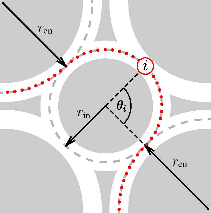
This paper considers the decision making of $n$ autonomous vehicles at a single-lane $w$-way unsignalised roundabout intersection. We assume that the vehicles do not communicate with each other, that entrances and exits of the roundabout are right-hand traffic, and that the traffic flows counter-clockwise within the roundabout. A vehicle may use any entrance and any exit of the roundabout but is not allowed to drive backward. Fig. 1 illustrates a four-way roundabout. We study the decision making based on vehicles within the roundabout and those approaching the roundabout, but independent of those that have already exited the roundabout.

In order to focus on the high-level decision making for autonomous vehicles, this paper does not consider the path trackers and the low-level control layer, which controls the engine to follow a precomputed navigation path (see Fig. 2). For this reason, we assume that a vehicle can perfectly follow a given navigation path.

A navigation path can be arbitrary as long as it is defined by a vehicle dynamic function that takes the current configuration and acceleration as arguments and returns the configuration in the next time step. Fig. 1 presents an example of a navigation path used in our experiment. In our framework, the configuration of a vehicle $i\in\{1,\ldots,n\}$ at time $t$ is given by:

where $r_{i}(t)$ and $\theta_{i}(t)$ indicate the position of the vehicle $i$ in polar coordinates, $v_{i}(t)$ is its speed (velocity along the path), and $s_{i}(t)\in\{\text{``enter'' },\text{``inside'' },\text{``exit''}\}$ is its status at time step $t$, respectively. Then, the time-evolution of the configuration of each vehicle $i$ is represented by

where the vehicle dynamic function $f_{i}$ returns the configuration of the vehicle $i$ after one time step, assuming that $a_{i}(t)$ is a constant acceleration along the path (the derivative of speed) between the time steps $t$ and $t+1$.

For example, in the case where the vehicle is within the roundabout (e.g., the vehicle $i$ in Fig. 1), $\bm{x}_{i}(t+1)=f_{i}(\bm{x}_{i}(t),a_{i}(t))$ is given by the dynamics as follows:

where $\Delta$ is the duration between two time steps. The cases where the vehicle is entering or exiting are similar.

Each vehicle decides its acceleration $a_{i}(t)$ at every time step $t$. To simplify the problem, we further assume that each vehicle $i$ chooses an acceleration $a_{i}(t)$ from a finite set at each time step $t$ to minimise their cost functions. This set of accelerations can theoretically be arbitrary, as long as it is finite. However, the larger this set is, the slower the computation of Nash equilibria will be. We provide concrete values in Section 5.

The goal of our paper is to design a process for decision making, which is a distributed algorithm to control the autonomous vehicles. The proposed decision-making process will be evaluated in Section 5 to ensure that multiple vehicles can operate simultaneously within a roundabout and can reach their target safely within an acceptable time.

Each vehicle computes its control input (namely, its acceleration) by trying to optimise not only its own objective but also its estimations of the objectives of the other vehicles. We define those objectives using cost functions, which specify how bad the situation is, considering two features: safety and speed. The safety feature is small when the distance with other vehicle is large, while the speed feature is small when the vehicle’s speed is close to the maximal legal speed. The trade-off is defined by the weight vector

where $w_{i}^{a}\geq 0$ is the weight of the speed feature, and $w_{i}^{s}=1-w_{i}^{a}\geq 0$ is the weight of the safety feature. This weight vector indicates how much the vehicle $i$ values speed over safety: the higher $w_{i}^{a}$ is (and so, the lower $w_{i}^{s}$ is), the more aggressive the vehicle will be (and so, the less conservative). Therefore, we call $w_{i}^{a}$ the aggressiveness of vehicle $i$. This value plays a significant role in our decision-making process.

We first introduce an overview of our proposed decision-making process (see also Fig. 3). Each vehicle $i$ repeats the following steps until it exits the roundabout.

1. 1.

   The vehicle $i$ observes the current configurations of its neighbours, which are the vehicles nearby (Section 3.2).

2. 2.

   The vehicle $i$ initialises the estimations of navigation paths and aggressiveness of the neighbours (Section 3.3) or updates those estimations by comparing the newly observed configurations with its predictions in the previous time step (Section 3.6).

3. 3.

   Based on the estimations, the vehicle $i$ computes its control input (acceleration) and predicts accelerations of its neighbours (Section 3.4).

4. 4.

   The vehicle $i$ predicts its neighbours’ future configurations up to a finite time horizon, based on the estimated navigation path and aggressiveness (Section 3.5).

5. 5.

   Then, the vehicle $i$ operates by using the computed control input and repeats the process for the next time step.

In the roundabout, each vehicle $i$ may not be able to observe all other vehicles, but only the vehicles nearby. Let $\mathcal{N}_{i}(t)\subseteq\{1,\ldots,m\}$ be the set of vehicles that are being observed by the vehicle $i$, called the neighbours of $i$, at time step $t$. We assume that $i\in\mathcal{N}_{i}(t)$ as $i$ can always observe itself. In our simulations, $\mathcal{N}_{i}(t)$ consists of $i$ itself, the closest two vehicles in front, and the closest one behind, if the distance is smaller than a fixed value $D$. The observation of $i$ at time $t$ is the collection of all the individual configurations $\bm{x}_{j}(t)$ for $j\in\mathcal{N}_{i}(t)$. We use $[\bm{x}_{j}(t)]_{j\in\mathcal{N}_{i}(t)}$ to denote the vector of observed configurations, also called observations, of all the neighbours of $i$.

Initially (at time step $t=0$), the vehicle $i$ estimates the aggressiveness $w_{j}^{a}$ of any vehicle $j\in\mathcal{N}_{i}(0)$ to be $\widehat{w^{a}_{i,j}}\langle 0\rangle=0.5$.

For the initial navigation paths, we cannot assume that the vehicle $i$ knows the vehicle dynamic function $f_{j}$ as $i$ does not know which path the vehicle $j$ will follow. For example, $i$ does not know which exit $j$ will use. Therefore, initially, the vehicle $i$ estimates a vehicle dynamic function $\widehat{f_{i,j}}\langle 0\rangle$ using the initial configuration $\bm{x}_{j}(0)$ of the vehicle $j$. Intuitively, if the vehicle $i$ detects that the vehicle $j$ is steering out, then it knows that $j$ will use the next exit. Otherwise, $i$ computes the navigation path as if the vehicle $j$ stayed within the roundabout indefinitely, possibly turning around several times. We always have $\widehat{f_{i,i}}\langle t\rangle=f_{i}$ at any time $t$ as $i$ knows its own navigation path.

We formulate a non-cooperative sequential game played between the vehicles to decide the acceleration at each time step (see Appendix for details). Each vehicle $i$ determines $a_{i}(t)$ at time $t$ using the Nash equilibrium of a sequential game

defined as follows.

1. 1.

   The players are the neighbours, i.e., elements of $\mathcal{N}_{i}(t)$.

2. 2.

   A strategy of each vehicle $j\in\mathcal{N}_{i}(t)$ is a vector of accelerations $\sigma_{j}=[a_{j}(t,\tau)]_{0\leq\tau<h}\in\Sigma$ for the time-step horizon from $\tau=0$ to $\tau=h-1$. Namely, $a_{j}(t,\tau)$ is an acceleration of the vehicle $j$ at time step $t+\tau$. Recall that $a_{j}(t,\tau)$ is selected from a finite set of accelerations (see Section 2.2). Therefore, the set $\Sigma$ of all possible strategies is also a finite set.

3. 3.

   Let $[\sigma_{j}]_{j\in\mathcal{N}_{i}(t)}$, where $\sigma_{j}\in\Sigma$, be a vector of strategies for all vehicles in $\mathcal{N}_{i}(t)$. The accumulated cost of vehicle $j\in\mathcal{N}_{i}(t)$ for the time horizon from $\tau=0$ to $\tau=h-1$ estimated by the vehicle $i$ at time $t$ is

   $\displaystyle\begin{split}\widehat{K_{i,j}}\langle t\rangle([\sigma_{k}&]_{k\in\mathcal{N}_{i}(t)})=\\ &\overline{K_{i,j}}\langle t\rangle(\mathcal{N}_{i}(t),\widehat{w^{a}_{i,j}}\langle t\rangle,[\sigma_{k}]_{k\in\mathcal{N}_{i}(t)}),\end{split}$

   (5)

   where the definition of the function $\overline{K_{i,j}}\langle t\rangle$ is given by Eq. (11) in Section 4. The objective of each vehicle playing this game is to minimise its accumulated cost.

4. 4.

   The order $\prec$ of the players in the sequential game is according to the estimated aggressiveness: if $\widehat{w^{a}_{i,j}}\langle t\rangle<\widehat{w^{a}_{i,k}}\langle t\rangle$, then $k$ makes the decision before $j$. In other words, the more aggressive a vehicle is, the more priority it will have to choose its control input (i.e., its acceleration).

Let $[\widetilde{a_{i,j}}\langle t,\tau\rangle]_{j\in\mathcal{N}_{i}(t),\,0\leq\tau<h}$ be a Nash equilibrium of this game, which always exists and is computable because the game is a finite perfect-information game O2009. Then, $\widetilde{a_{i,j}}\langle t,\tau\rangle$ is the acceleration of the vehicle $j$ at time $t+\tau$ that vehicle $i$ predicts at time $t$. We compute this Nash equilibrium using backward induction (see Appendix for details). The theoretical complexity of this computation is $O(h\cdot\lvert\mathcal{N}_{i}(t)\rvert\cdot\lvert\Sigma\rvert^{\mathcal{N}_{i}(t)})$. Observe that this complexity is exponential in the number of players, which explains why we restrict these games to be played only among neighbours.

Finally, we use $\widetilde{a_{i,i}}\langle t,0\rangle$ as the control input of vehicle $i$ at time step $t$.

For each vehicle $j\in\mathcal{N}_{i}(t)$, let $\bm{a}_{j}=[a_{j}(t,\tau)]_{0\leq\tau<h}$ be a given vector of accelerations of $j$. For example, those accelerations can be a Nash equilibrium computed in Section 3.4, namely, $\bm{a}_{j}=[\widetilde{a_{i,j}}\langle t,\tau\rangle]_{0\leq\tau<h}$.

Let $\overline{\bm{x}_{i,j}}\langle t,\tau\rangle(\bm{a}_{j})$ be the configuration of the vehicle $j$ that would be reached at time step $t+\tau$, based on the observation $\bm{x}_{j}(t)$, the estimations $\widehat{f_{i,j}}\langle t\rangle$, and the vector of accelerations $\bm{a}_{j}$. These configurations are computed by induction as follows.

• •

  The configuration at time step $t$ is the observed configuration

  $$\overline{\bm{x}_{i,j}}\langle t,0\rangle(\bm{a}_{j})=\bm{x}_{j}(t).$$

  (6)

• •

  The configuration at time step $t+\tau+1$ is computed by assuming that the vehicle $j$ will follow the estimated navigation path computed using $\widehat{f_{i,j}}\langle t\rangle$, from the configuration $\overline{\bm{x}_{i,j}}\langle t,\tau\rangle(\bm{a}_{j})$, with acceleration $a_{j}(t,\tau)$:

  $$\overline{\bm{x}_{i,j}}\langle t,\tau+1\rangle(\bm{a}_{j})=\widehat{f_{i,j}}\langle t\rangle\Bigl(\overline{\bm{x}_{i,j}}\langle t,\tau\rangle(\bm{a}_{j}),a_{j}(t,\tau)\Bigr).$$

  (7)

In particular, we define the predicted configuration of the vehicle $j$ at time $t+\tau$ which vehicle $i$ predicts at time $t$ as

At each time step $t$, let $U_{i}(t)\subseteq\mathcal{N}_{i}(t)\setminus\{i\}$ be the set of vehicles such that the distance between the observed configuration $\bm{x}_{j}(t+1)$ and the predicted configuration $\widetilde{\bm{x}_{i,j}}\langle t,1\rangle$ is bigger than a fixed value. Since the predictions of the vehicle $i$ are not precise, $i$ needs to update its estimations of aggressiveness and navigation path for each vehicle $j\in U_{i}(t)$.

For the aggressiveness, the vehicle $i$ updates the estimation $\widehat{w^{a}_{i,j}}\langle t\rangle$ to $\widehat{w^{a}_{i,j}}\langle t+1\rangle$, which describes the behaviour of the vehicle $j$ more accurately. The vehicle $i$ considers each value $w^{a}$ in a given fixed finite set $\mathcal{W}$ and constructs a game $G_{i,j}(t,w^{a})$ in the same way as $G_{i}(t)$ in Section 3.4. Concretely, we construct $G_{i,j}(t,w^{a})$ as follows.

1. 1.

   The set of players is $\{i,j\}$.

2. 2.

   The strategies are the same as in Section 3.4.

3. 3.

   Given strategies $\sigma_{i}$ and $\sigma_{j}$ for the vehicles $i$ and $j$ respectively, their accumulated cost for every vehicle $l\in\{i,j\}$ in this game is

   $$\overline{K_{i,l}}\langle t\rangle(\{i,j\},w^{a},[\sigma_{k}]_{k\in\{i,j\}}),$$

   (9)

   where $\overline{K_{i,l}}\langle t\rangle$ is the same function as in Section 3.4, and which will be described in Section 4.

4. 4.

   The order $\prec$ of players is defined in the same way as in Section 3.4.

Let $[\overline{a_{k}}\langle t,\tau\rangle(w^{a})]_{k\in\{i,j\},\,0\leq\tau<h}$ denotes the Nash equilibrium of this new game $G_{i,j}(t,w^{a})$. Then, the vehicle $i$ computes a new estimated aggressiveness $\widehat{w^{a}_{i,j}}\langle t+1\rangle$ of the vehicle $j$ that fits the observed acceleration $a_{j}(t+1)$ the most closely, i.e.,

Otherwise, if the predicted configuration is close enough to the observed configuration ($j\notin U_{i}(t)$), then $\widehat{w^{a}_{i,j}}\langle t+1\rangle=\widehat{w^{a}_{i,j}}\langle t\rangle$. The estimated vehicle dynamic function $\widehat{f_{i,j}}\langle t\rangle$ is updated in the same way as in Section 3.3.

In this section, we consider the situation where all vehicles in $\mathcal{N}_{i}(t)$ are stopped, that is, have zero speed. This situation is particularly critical, as it may induce a deadlock: every vehicle is waiting for the other vehicles to move.

In this case, we want the vehicle $i$ to make a move, as long as it is not in a critical situation, i.e., the situation when $i$ is waiting to enter the roundabout but observes that a vehicle is already inside the roundabout. If the vehicle $i$ is not in such a critical situation, we enforce it to make a move by setting the acceleration $a_{i}(t)$ to $10\,ms^{-2}$ with probability $0.5$.

We construct the accumulated cost using the receding horizon control approach K2005, based on the predicted future up to a horizon time step $h<\infty$. Recall that we use this accumulated cost to determine the control inputs of each vehicle $i$ in Section 3.4, and to update the estimation of the aggressiveness of other vehicles in Section 3.6.

As introduced in Section 3.4, a strategy of each vehicle $j\in\mathcal{N}$ is a vector of accelerations $\sigma_{j}=[a_{j}(t,\tau)]_{0\leq\tau<h}$ for the time-step horizon from $\tau=0$ to $\tau=h-1$. The accumulated cost function of the vehicle $j$, computed by the vehicle $i$ at time step $t$, based on the aggressiveness value $w^{a}$ is

where $\lambda\in(0,1)$ is a fixed discount factor, $[\overline{\bm{x}_{i,k}}\langle t,\tau\rangle(\sigma_{k})]_{k\in\mathcal{N}}$ is the predicted configuration at time step $t+\tau$ that was defined in Section 3.5, and $S_{j}$ is the time-step cost function that will be defined in Section 4.2.

Let us remark that the vehicle $i$ uses its own observations to compute the accumulated cost of the vehicle $j$. Specifically, in Eq. (5), $i$ computes the accumulated cost of $j$ using its own neighbours $\mathcal{N}_{i}(t)$. In the case where $j$ is the nearest vehicle in front of $i$, we have two situations depending on whether or not $i$ can observe its second nearest vehicle in front. If it can, then this vehicle will be in $\mathcal{N}_{i}(t)$ and will be considered as the nearest vehicle in front of $j$ in the computation of $\overline{K_{i,j}}\langle t\rangle$. If it cannot, this means that the second nearest vehicle is too far from $i$, so that $i$ will compute $\overline{K_{i,j}}\langle t\rangle$ as if there were no vehicle in front of $j$.

We introduce the cost of a vehicle at each time step that we call time-step cost and use it for computing the accumulated cost in Eq. (11). The time-step cost function of the vehicle $i$ is given by

where $[\bm{x}_{j}]_{j\in\mathcal{N}}$ is a given vector of configurations of vehicles in $\mathcal{N}$, $\phi_{i}^{\text{safe}}$ and $\phi_{i}^{\text{speed}}$ are safety and speed features defined in Sections 4.2.1 and 4.2.2, respectively.

The roundabout and the navigation paths used in the simulation shown in Fig. 4 are designed based on practical situations anjana2014development. All vehicles drive on the right-hand side of the road and enter the roundabout using one of the four entrances. The road occupancy of a vehicle is modelled as a circle with diameter $4.5m$.

The vehicle dynamics is as in Eq. (3) with time interval $\Delta=0.25s$ (following li18 and tian18). The status of a vehicle entering (resp. exiting) the roundabout changes from “enter” to “inside” (resp. “inside” to “exit”) when the distance between its centre and the centre of the roundabout is at least (resp. greater than) $r_{\text{in}}+4.5m$, i.e., when it can (resp. cannot) possibly collides with other vehicles inside the roundabout. In Fig. 4, vehicles $1$ and $3$ are at the status-changing positions.

We perform simulations by considering four to eight vehicles, whose types of navigation paths are determined randomly. The initial positions of the vehicles are shown in Fig. 4. The initial speeds are randomly selected from $[0,v_{l}]$, where $v_{l}=11ms^{-1}$ is the speed limit of the road fha. The aggressiveness $w_{i}^{a}$ of each vehicle $i$ is randomly selected from $\{0.2,0.3,\ldots,0.8\}$. Table 5.1 presents the setting of parameters. In addition, we use the following vectors of acceleration/deceleration sequences for the strategies of the sequential game (the strategies in $\Sigma$, see Section 3.4) with a time horizon $h=4$ (the unit is $m/s^{2}$).

• •

  $\begin{bmatrix}-50&0&0&0&0\end{bmatrix}$ for a strong deceleration,

• •

  $\begin{bmatrix}-10&0&0&0&0\end{bmatrix}$ for a small deceleration,

• •

  $\begin{bmatrix}0&0&0&0&0\end{bmatrix}$ for no acceleration,

• •

  $\begin{bmatrix}10&0&0&0&0\end{bmatrix}$ for a small acceleration,

• •

  $\begin{bmatrix}30&0&0&0&0\end{bmatrix}$ for a strong acceleration.

To update the estimation of the aggressiveness (see Section 3.6), we use $\mathcal{W}=\{0.1,\ldots,0.9\}$, although the actual aggressiveness $w^{a}_{j}$ of each vehicle $j$ is initialised within the range $\{0.2,0.3,\ldots,0.8\}$. We allow a vehicle $i$ to update an estimated aggressiveness $\widehat{w^{a}_{i,j}}\langle t\rangle$ to be $0.1$ and $0.9$ (see Section 3.6) so that $i$ can determine whether $\widehat{w^{a}_{i,i}}\langle t\rangle<\widehat{w^{a}_{i,j}}\langle t\rangle$ or $\widehat{w^{a}_{i,i}}\langle t\rangle>\widehat{w^{a}_{i,j}}\langle t\rangle$. Therefore, $i$ can decide the order of the players for the sequential game in Section 3.4.

All the programs were coded and run using MATLAB 2018a and MATLAB 2018b.

References

- [1] Kaur, K., Rampersad, G.: ‘Trust in driverless cars: Investigating key factors influencing the adoption of driverless cars’, Journal of Engineering and Technology Management, 2018, 48, pp. 87–96
- [2] Schwarting, W., Alonso-Mora, J., Rus, D.: ‘Planning and decision-making for autonomous vehicles’, Annual Review of Control, Robotics, and Autonomous Systems, 2018,
- [3] Liu, X., Cao, P., Xu, Z., Fan, Q.: ‘Analysing driving efficiency of mandatory lane change decision for autonomous vehicles’, IET Intelligent Transport Systems, 2018, 13
- [4] Chentong, B., Yin, G., Xu, L., Zhang, N.: ‘Active collision algorithm for autonomous electric vehicles at intersections’, IET Intelligent Transport Systems, 2018, 13
- [5] Galceran, E., Cunningham, A.G., Eustice, R.M., Olson, E. ‘Multipolicy decision-making for autonomous driving via changepoint-based behavior prediction’. In: Robotics: Science and Systems. (Rome, Italy, 2015). pp. 1–10
- [6] Perez, J., Milanes, V., Onieva, E., Godoy, J., Alonso, J. ‘Longitudinal fuzzy control for autonomous overtaking’. In: 2011 IEEE International Conference on Mechatronics. (Istanbul, Turkey, 2011). pp. 188–193
- [7] Gipps, P.G.: ‘A model for the structure of lane-changing decisions’, Transportation Research Part B: Methodological, 1986, 20, (5), pp. 403–414
- [8] Wang, J., Zhang, Q., Zhao, D., Chen, Y. ‘Lane change decision-making through deep reinforcement learning with rule-based constraints’. In: 2019 IEEE International Joint Conference on Neural Networks (IJCNN). (Budapest, Hungary, 2019). pp. 1–6
- [9] Zimmerman, N., Schlenoff, C., Balakirsky, S. ‘Implementing a rule-based system to represent decision criteria for on-road autonomous navigation’. In: 2004 AAAI Spring Symposium on Knowledge Representation and Ontologies for Autonomous Systems. (California, USA, 2004). pp. 1–5
- [10] Qiao, Z., Muelling, K., Dolan, J.M., Palanisamy, P., Mudalige, P. ‘Automatically generated curriculum based reinforcement learning for autonomous vehicles in urban environment’. In: 2018 IEEE Intelligent Vehicles Symposium (IV). (Changshu, China, 2018). pp. 1233–1238
- [11] Liu, Y., Wang, X., Li, L., Cheng, S., Chen, Z.: ‘A novel lane change decision-making model of autonomous vehicle based on support vector machine’, IEEE Access, 2019, 7, pp. 26543–26550
- [12] Li, X., Xu, X., Zuo, L. ‘Reinforcement learning based overtaking decision-making for highway autonomous driving’. In: 2015 IEEE Sixth International Conference on Intelligent Control and Information Processing (ICICIP). (Wuhan, China, 2015). pp. 336–342
- [13] You, C., Lu, J., Filev, D., Tsiotras, P. ‘Highway traffic modeling and decision making for autonomous vehicle using reinforcement learning’. In: 2018 IEEE Intelligent Vehicles Symposium (IV). (Changshu, China, 2018). pp. 1227–1232
- [14] Xu, X., Zuo, L., Li, X., Qian, L., Ren, J., Sun, Z.: ‘A reinforcement learning approach to autonomous decision making of intelligent vehicles on highways’, IEEE Transactions on Systems, Man, and Cybernetics: Systems, 2018,
- [15] Hoel, C.J., Wolff, K., Laine, L. ‘Automated speed and lane change decision making using deep reinforcement learning’. In: 2018 IEEE 21st International Conference on Intelligent Transportation Systems (ITSC). (Hawaii, USA, 2018). pp. 2148–2155
- [16] Li, X., Cao, C.C., Shi, Y., Bai, W., Gao, H., Qiu, L., et al.: ‘A survey of data-driven and knowledge-aware explainable ai’, IEEE Transactions on Knowledge and Data Engineering, 2020, pp. 1–1
- [17] Glomsrud, J., Ødegårdstuen, A., Clair, A., Smogeli, O. ‘Trustworthy versus explainable ai in autonomous vessels’. In: International Seminar on Safety and Security of Autonomous Vessels (ISSAV). (Espoo, Finland, 2019).
- [18] Yu, H., Tseng, H.E., Langari, R.: ‘A human-like game theory-based controller for automatic lane changing’, Transportation Research Part C: Emerging Technologies, 2018, 88, pp. 140–158
- [19] Albaba, B.M., Yildiz, Y.: ‘Driver modeling through deep reinforcement learning and behavioral game theory’, arXiv preprint arXiv:200311071, 2020,
- [20] Talebpour, A., Mahmassani, H.S., Hamdar, S.H.: ‘Modeling lane-changing behavior in a connected environment: A game theory approach’, Transportation Research Part C: Emerging Technologies, 2015, 59, pp. 216–232
- [21] Li, N., Zhang, M., Yildiz, Y., Kolmanovsky, I., Girard, A. ‘Game theory-based traffic modeling for calibration of automated driving algorithms’. In: Control Strategies for Advanced Driver Assistance Systems and Autonomous Driving Functions. vol. 476 of Lecture Notes in Control and Information Sciences. (Springer, 2019). pp. 89–106
- [22] Li, N., Kolmanovsky, I., Girard, A., Yildiz, Y. ‘Game theoretic modeling of vehicle interactions at unsignalized intersections and application to autonomous vehicle control’. In: 2018 IEEE Annual American Control Conference (ACC). (USA, 2018). pp. 3215–3220
- [23] Elhenawy, M., Elbery, A.A., Hassan, A.A., Rakha, H.A. ‘An intersection game-theory-based traffic control algorithm in a connected vehicle environment’. In: 2015 IEEE 18th International Conference on Intelligent Transportation Systems. (Spain, 2015). pp. 343–347
- [24] Wei, H., Mashayekhy, L., Papineau, J. ‘Intersection management for connected autonomous vehicles: A game theoretic framework’. In: 2018 21st International Conference on Intelligent Transportation Systems (ITSC). (Hawaii, USA, 2018). pp. 583–588
- [25] Banjanovic.Mehmedovic, L., Halilovic, E., Bosankic, I., Kantardzic, M., Kasapovic, S.: ‘Autonomous vehicle-to-vehicle (v2v) decision making in roundabout using game theory’, Int J Adv Comput Sci Appl, 2016, 7, pp. 292–298
- [26] Tian, R., Li, S., Li, N., Kolmanovsky, I., Girard, A., Yildiz, Y. ‘Adaptive game-theoretic decision making for autonomous vehicle control at roundabouts’. In: 2018 IEEE Conference on Decision and Control (CDC). (USA, 2018). pp. 321–326
- [27] Deluka.Tibljaš, A., Giuffrè, T., Surdonja, S., Trubia, S.: ‘Introduction of autonomous vehicles: Roundabouts design and safety performance evaluation’, Sustainability, 2018, 10, (4), pp. 1060
- [28] Manage, S., Nakamura, H., Suzuki, K., et al.: ‘Performance analysis of roundabouts as an alternative for intersection control in Japan’, Journal of the Eastern Asia Society for Transportation Studies, 2003, 5, pp. 871–883
- [29] Wang, W., Meng, Q., Chung, P.W.H. ‘Camera based decision making at roundabouts for autonomous vehicles’. In: 2018 IEEE 15th International Conference on Control, Automation, Robotics and Vision (ICARCV). (Singapore, 2018). pp. 1460–1465
- [30] Wang, W., Nguyen, Q.A., Ma, W., Wei, J., Chung, P.W.H., Meng, Q. ‘Multi-grid based decision making at roundabout for autonomous vehicles’. In: 2019 IEEE International Conference of Vehicular Electronics and Safety (ICVES). (Cairo, Egypt, 2019). pp. 1–6
- [31] García Cuenca, L., Puertas, E., Fernandez Andrés, J., Aliane, N.: ‘Autonomous Driving in Roundabout Maneuvers Using Reinforcement Learning with Q-Learning’, Electronics, 2019, 8, (12), pp. 1536
- [32] Pérez, J., González, C., Milanés, V., Onieva, E., Godoy, J., de Pedro, T. ‘Modularity, adaptability and evolution in the autopia architecture for control of autonomous vehicles’. In: 2009 IEEE International Conference on Mechatronics. (Malaga, Spain, 2009). pp. 1–5
- [33] Liu, S., Li, L., Tang, J., Wu, S., Gaudiot, J.L.: ‘Creating Autonomous Vehicle Systems’. (Morgan & Claypool Publishers, 2017)
- [34] Osborne, M.J.: ‘An introduction to game theory’. (Oxford University Press, 2004)
- [35] H..Kwon, W., Han, S.: ‘Receding Horizon Control: Model Predictive Control for State Models’. (Springer, 2005)
- [36] Anjana, S., Anjaneyulu, M.V.L.R.: ‘Development of safety performance measures for urban roundabouts in india’, Journal of Transportation Engineering, 2014, 141, (1), pp. 4001–4066
- [37] Li, N., Kolmanovsky, I., Girard, A., Yildiz, Y. ‘Game Theoretic Modeling of Vehicle Interactions at Unsignalized Intersections and Application to Autonomous Vehicle Control’. In: 2018 IEEE Annual American Control Conference (ACC). (WI, USA, 2018). pp. 3215–3220
- [38] Tian, R., Li, S., Li, N., Kolmanovsky, I., Girard, A., Yildiz, Y. ‘Adaptive Game-Theoretic Decision Making for Autonomous Vehicle Control at Roundabouts’. In: Proceedings of the 2018 IEEE Conference on Decision and Control (CDC). (FL, USA, 2018). pp. 321–326
- [39] Federal Highway Administration. ‘Roundabouts and mini roundabouts’, 2020. Available at: https://safety.fhwa.dot.gov/intersection/innovative/roundabouts/
Appendix: 1-round sequential game with perfect information
In this section, we give a detailed explanation of the sequential game in Section 3.4. At each time step , each vehicle considers a -round sequential game
where is the set of players, is the set of all possible strategies for each player, and is the function in Eq. (5), and is an order of players.
Let . A vector of strategies is called a best response of player , , if
for any strategy . The strategy profile is also called a Nash equilibrium if it is a best response of all players. In other words, a Nash equilibrium is a strategy profile such that no player can reduce her cost by changing her strategy, provided that all other players do not change theirs.
The players take turns selecting their strategies according to the order – meaning that if then selects her strategy before – and the game stops after all players have selected their strategies. A sequential game is a game with perfect information if each player remembers the history of all strategies played before her. In Section 3.4, this order is determined by the estimations of aggressiveness.
The extensive-form of a -round sequential game with perfect and complete information can be described as a finite decision tree. Fig. 8 shows an extensive-form of such a game played between two players. As we assume that , selects her strategy before at the root of the tree. We can obtain a Nash equilibrium of the game by applying the backward induction algorithm on the decision tree. For the game in Fig. 8, we can compute a Nash equilibrium as follows. First, we compute best responses for in both subtrees, which represent the cases that selects and . If selects (resp. ), then (resp. ) is a best response for . We then compute the best response for by considering the best responses of for each subtree. In this case, is a Nash equilibrium.
The extensive-form of the game is a tree with the branching of and is deep. Consequently, it has nodes. Each node requires the computation of an accumulated cost. The complexity of this computation is , because, for every time step until the horizon, we have to compute and . In conclusion, the complexity of this backward induction is .
We invite interested readers to see textbooks (e.g. O2009) for more details on game theory.