A robust approach to model-based classification based on trimming and constraints
Semi-supervised learning in presence of outliers and label noise
Abstract
In a standard classification framework a set of trustworthy learning data are employed to build a decision rule, with the final aim of classifying unlabelled units belonging to the test set. Therefore, unreliable labelled observations, namely outliers and data with incorrect labels, can strongly undermine the classifier performance, especially if the training size is small. The present work introduces a robust modification to the Model-Based Classification framework, employing impartial trimming and constraints on the ratio between the maximum and the minimum eigenvalue of the group scatter matrices. The proposed method effectively handles noise presence in both response and exploratory variables, providing reliable classification even when dealing with contaminated datasets. A robust information criterion is proposed for model selection. Experiments on real and simulated data, artificially adulterated, are provided to underline the benefits of the proposed method.
1 Introduction
In statistical learning, we define classification as the task of assigning group memberships to a set of unlabelled observations. Whenever a labelled sample (i.e., the training set) is available, the information contained in such dataset is exploited to classify the remaining unlabelled observations (i.e., the test set), either in a supervised or in a semi-supervised manner, depending whether the information contained in the test set are included in building the classifier (McNicholas 2016, e.g.). Either way, the presence of unreliable data points can be detrimental for the classification process, especially if the training size is small (Zhu and Wu 2004).
Broadly speaking, noise is anything that obscures the relationship between the attributes and the class membership (Hickey 1996). In a classification context, Wu 1995 distinguishes between two types of noise: attribute noise and class noise. The former is related to contamination in the exploratory variables, that is when observations present unusual values on their predictors; whereas the latter refers to samples whose associated labels are wrong. Zhu and Wu 2004 and the recent work of Prati et al. 2018 offer an extensive review on the topic and the methods that have been proposed in the literature to deal with attribute noise and class noise, respectively. Generally, three main approaches can be employed when building a classifier from a noisy dataset: cleaning the data, modeling the noise and using robust estimators of model parameters (Bouveyron and Girard 2009).
The approach presented in this paper is based on a robust estimation of a Gaussian mixture model with parsimonious structure, to account for both attribute and label noise. Our conjecture is that the contaminated observations would be the least plausible units under the robustly estimated model: the corrupted subsample will be revealed by detecting those observations with the lowest contributions to the associated likelihood. Impartial trimming (Gordaliza 1991a; Gordaliza 1991b; Cuesta-Albertos et al. 1997) is employed for robustifying the parameter estimates, being a well established technique to treat mild and gross outliers in the clustering literature (García-Escudero et al. 2010) and here used, for the first time, to additionally account for label noise in a classification framework. A semi-supervised approach is developed, where information contained in both labelled and unlabelled samples is combined for improving the classifier performance and for defining a data-driven method to identify outlying observations possibly present in the test set.
The rest of the manuscript is organized as follows. A brief review on model-based discriminant analysis and classification is given in Section 2, Section 3 introduces the robust updating classification rules, covering the model formulation, inference aspects and model selection. Simulation studies to compare the method introduced in Section 3 with other popular classification methods are reported in Section 4. Finally, in Section 5 our proposal is employed in performing classification and adulteration detection in a food authenticity context, dealing with contaminated samples of Irish honey. Concluding notes and further research directions are outlined in Section 6. The proof of Proposition 1, details on the parameters values for simulation study II and efficient algorithms for enforcing the eigen-ratio constraint for different patterned models are deferred respectively to appendices A, B and C.
2 Model-Based Discriminant Analysis and Classification
In this Section we review the main concepts of supervised classification based on mixture models, with particular focus on Eigenvalue Decomposition Discriminant Analysis and its semi-supervised formulation, as introduced in Dean et al. 2006. This approach is the basis of the novel robust semi-supervised classifier introduced in Section 3.
2.1 Eigenvalue Decomposition Discriminant Analysis
Model-based discriminant analysis (McLachlan 1992; Fraley and Raftery 2002) is a probabilistic approach for supervised classification, in which a classifier is built from a complete set of learning observations ; where and , , are independent realizations of random vectors and , respectively. That is, denotes a -variate observation and its associated class label, such that if observation belongs to group and otherwise, . Considering a Gaussian framework, the probabilistic mechanism that is assumed to have generated the data is as follows:
| (1) | ||||
where is multinomially distributed with probability of observing class and the conditional density of given is multivariate normal with mean vector and variance covariance matrix . Therefore, the joint density of is given by:
| (2) |
where denotes the multivariate normal density and represents the collection of parameters to be estimated, . Discriminant analysis makes use of data with known labels to estimate model parameters for creating a classification rule. The trained classifier is subsequently employed for assigning a set of unlabelled observations , to the class with the associated highest posterior probability:
| (3) |
using the maximum a posteriori (MAP) rule. The afore-described framework is widely employed in classification tasks, thanks to its probabilistic formulation and well-established efficacy.
The number of parameters in the component variance covariance matrices grows quadratically with the dimension . Thus, Bensmail and Celeux 1996 introduced a parsimonious parametrization proposing to enforce additional assumptions on the matrices structure, based on the eigen-decomposition of Banfield and Raftery 1993 and Celeux and Govaert 1995:
| (4) |
where is an orthogonal matrix of eigenvectors, is a diagonal matrix such that and . This elements correspond respectively to the orientation, shape and volume (alternatively called scale) of the different Gaussian components. Allowing each parameter in (4) to be equal or different across groups, Bensmail and Celeux 1996 define a family of 14 patterned models, listed in Table 1. Such class of models is particularly flexible, as it includes very popular classification methods like Linear Discriminant Analysis and Quadratic Discriminant Analysis as special cases for the EEE and VVV models, respectively (Hastie and Tibshirani 1996). Eigenvalue Decomposition Discriminant Analysis (EDDA) is implemented in the mclust R package (Fop et al. 2016).
| Model | ER | |||
|---|---|---|---|---|
| EII | - | Not required | ||
| VII | - | Required | ||
| EEI | - | Not required | ||
| VEI | - | Required | ||
| EVI | - | Required | ||
| VVI | - | Required | ||
| EEE | Not required | |||
| VEE | Required | |||
| EVE | Required | |||
| EEV | Not required | |||
| VVE | Required | |||
| VEV | Required | |||
| EVV | Required | |||
| VVV | Required |
2.2 Updating Classification Rules
Exploiting the assumption that the data generating process outlined in (1) is the same for both labelled and unlabelled observations, Dean et al. 2006 propose to include also the data whose memberships are unknown in the parameter estimation. That is, information about group structure that may be contained in both labelled and unlabelled samples is combined in order to improve the classifier performance, in a semi-supervised manner.
Under the framework defined in Section 2.1, and given the set of available information , the observed log-likelihood is
| (5) | ||||
in which both labelled and unlabelled samples are accounted for in the likelihood definition. Treating the (unknown) labels , , as missing data and including them in the likelihood specification defines the so called complete-data log-likelihood:
| (6) | ||||
Maximum likelihood estimates for (5) are obtained through the EM algorithm (Dempster et al. 1977), iteratively computing the expected value for the unknown labels given the current set of parameter estimates (E-Step), and employing (6) to find maximum likelihood estimates for the unknown parameters (M-Step). The unlabelled data are then classified according to , using the MAP. The updating classification rules was demonstrated to give improved classification performance over the classical model-based discriminant analysis in some food authenticity applications, particularly when the training size is small. An implementation of this can be found in the upclass R package (Russell et al. 2014).
3 Robust Updating Classification Rules
We introduce here a Robust modification to the Updating Classification Rule described in Section 2.2, with the final aim of developing a classifier whose performance is not affected by contaminated data, either in the form of label noise and outlying observations.
3.1 Model Formulation
The main idea of the proposed approach is to employ techniques originated in the branch of robust statistics to obtain a model-based classifier in which parameters are robustly estimated and outlying observations identified. We are interested in providing a method that jointly accounts for noise on response and exploratory variables, where the former might be present in the labelled set and the latter in both the labelled and unlabelled sets. We propose to modify the log-likelihood in (5) with a trimmed mixture log-likelihood (Neykov et al. 2007) and to employ impartial trimming and constraints on the covariance matrices for achieving both robust parameter estimation and identification of the unreliable sub-sample. Impartial trimming is enforced by considering the distinct structure of the likelihoods associated to the labelled and unlabelled sets, accounting for the possible label noise that might be present in the labelled sample (see Section 3.2 for details). Following the same notation introduced in Section 2.1, we aim at maximizing the trimmed observed data log-likelihood:
| (7) | ||||
where , are 0-1 trimming indicator functions, that express whether observation and are trimmed off or not. A fixed fraction and of observations, belonging to the labelled and unlabelled set respectively, is unassigned by setting and . In this way, the less plausible samples under the currently estimated model are tentatively trimmed out at each step of the iterations that leads to the final estimate. The labelled trimming level and the unlabelled trimming level account for possible adulteration in both sets. At the end of the iterations, a value of or corresponds to identify or , respectively, as unreliable observations. Notice that impartial trimming automatically deals with both class noise and attribute noise, as observations that suffer from either noise structure will give low contribution to the associated likelihood.
Maximization of (7) is carried out via the EM algorithm, in which an appropriate Concentration Step (Rousseeuw and Driessen 1999) is performed in both labelled and unlabelled sets at each iteration to enforce the impartial trimming. In addition, we protect the parameter estimation from spurious solutions, that may arise whenever one component of the mixture fits a random pattern in the data. We consider the eigenvalue-ratio restriction:
| (8) |
where and , with , being the eigenvalues of the matrix and being a fixed constant (Ingrassia 2004). Constraint (8) simultaneously controls differences between groups and departures from sphericity, by forcing the relative length of the axes of the equidensity ellipsoids, based on the multivariate normal distribution, to be smaller than (García-Escudero et al. 2014). Notice that the constraint in (8) is still needed whenever either the shape or the volume is free to vary across components (García-Escudero et al. 2017), that is for all models in Table 1 that present “Required” entry in the ER column. The considered approach is the (semi)-supervised version of the methodology proposed in Dotto and Farcomeni 2019, which is framed in a completely unsupervised scenario. Feasible and computationally efficient algorithms for enforcing the eigen-ratio constraint for different patterned models are reported in the Appendix C.
3.2 Estimation Procedure
The EM algorithm for obtaining Maximum Trimmed Likelihood Estimates of the robust updating classification rule involves the following steps:
- •
Robust Initialization: set . Employing only the labelled data, we obtain robust starting values for the mean vector and covariance matrix of the multivariate normal density for each group , , employing the following procedure:
- 1.
For each class , draw a random -subset and compute its empirical mean and variance covariance matrix according to the considered parsimonious structure. This procedure yields better initial subsets than drawing random -subsets directly, because the probability of drawing an outlier-free -subset is much higher than that of drawing an outlier-free -subset (Hubert et al. 2018).
- 2.
Set
where .
- 3.
For each , , compute the conditional density
(9) of the samples with lowest value of (9) are temporarily discarded as possible outliers, namely label noise and/or attribute noise. That is, for such observations.
- 4.
The parameter estimates are updated, based on the non-discarded observations:
(10) (11) Estimation of depends on the considered patterned model, details are given in Bensmail and Celeux 1996.
- 5.
Iterate until the discarded observations are exactly the same on two consecutive iterations, then stop (usually, iterations are required).
The procedure described in steps is performed nsamp times, and the parameter estimates that lead to the highest value of the objective function , out of nsamp repetitions, are retained. The afore-described procedure stems from the ideas of the FastMCD algorithm of Rousseeuw and Driessen 1999, here adapted for dealing with parsimonious structures in the covariance matrices. Retaining as final estimates leads to a fully supervised robust model-based method, called REDDA hereafter (see Section 4.1.1). Then, if the selected patterned model allows for heteroscedastic and (8) is not satisfied, constrained maximization is enforced, see Appendix C for details.
- 1.
- •
EM Iterations: denote by the parameter estimates at the -th iteration of the algorithm.
- –
Step 1 - Concentration: the trimming procedure is implemented by discarding the observations with smaller values of
(12) and discarding the observations with smaller values of
(13) - –
Step 2 - Expectation: for each non-trimmed observation compute the posterior probabilities
(14) - –
Step 3 - Constrained Maximization: the parameter estimates are updated, based on the non-discarded observations and the current estimates for the unknown labels:
(15) (16) Estimation of depends on the considered patterned model and on the eigenvalues-ratio constraint. Details are given in Bensmail and Celeux 1996 and, if (8) is not satisfied, in Appendix C.
- –
Step 4 - Convergence of the EM algorithm: check for algorithm convergence (see Section 3.3). If convergence has not been reached, set and repeat steps 1-4.
- –
Notice how the trimming step differs between the labelled and unlabelled observations. We implicitly assume that a label in the training set conveys a sound meaning about the presence of a class of objects. Therefore, in the labelled set, we opted for trimming the samples with lowest conditional density . The alternative choice of considering the joint density is instead prone to trim off completely groups with small prior probability for large enough value of , and should be discarded. Note that with (12) we are both discriminating label noise (i.e., observations that are likely to belong to the mixture model but whose associated label is wrong) and outliers. In the unlabelled set, on the other hand, trimming is based on the marginal density , having no prior information on the group membership of the samples.
Once convergence is reached, the estimated values provide a classification for the unlabelled observations , assigning observation into group if for all . Final values of , and , classify and respectively, as outlying observations.
The routines for estimating the robust updating classification rules have been written in R language (R Core Team 2018): the source code is available at https://github.com/AndreaCappozzo/rupclass.
The estimation procedure detailed in this Section implies the monotonicity of the algorithm, according to:
Proposition 1: If the values , , , are kept fixed, the EM algorithm described in Section 3.2 implies at any .
The proof is reported in Appendix A. Furthermore, our estimation procedure reduces possible incorrect modes of the optimization function (spurious maximizers) and offers a constructive way to obtain a maximizer for the sample problem, that converges to the global maximizer for the population, see García-Escudero et al. 2008 and García-Escudero et al. 2015.
3.3 Convergence Criterion
We assess whether the EM algorithm has reached convergence evaluating at each iteration how close the trimmed log-likelihood is to its estimated asymptotic value, using the Aitken acceleration (Aitken 1926):
| (17) |
where is the trimmed observed data log-likelihood from iteration . The asymptotic estimate of the trimmed log-likelihood at iteration is given by (Bohning et al. 1994):
| (18) |
The EM algorithm is considered to have converged when ; a value of has been chosen for the experiments reported in the next Sessions.
3.4 Model Selection
A robust likelihood-based criterion is employed for choosing the best model among the 14 patterned covariance structures listed in Table 1 and a reasonable value for the constraint in (8):
| (19) |
where denotes the maximized trimmed observed data log-likelihood and a penalty term whose definition is:
| (20) |
That is, depends on the total number of parameters to be estimated: and for every patterned model are given in Table 1. It also accounts for the trimming levels and for the eigen-ratio constraint , according to Cerioli et al. 2018. Note that, when and , (19) is the Bayesian Information Criterion (Schwarz 1978).
4 Simulation studies
In this Section, we present two simulated data experiments: Simulation Study I compares the performances of several model-based classification methods in a low dimensional setting when dealing with noisy data at different contamination rates; Simulation Study II considers a higher dimensional scenario in which the accuracy performance of some popular classification methods is assessed, at a fixed contamination rate. In both scenarios we consider a joint noise structure on response and exploratory variables.
4.1 Simulation Study I
4.1.1 Experimental Setup
We consider a data generating process given by a mixture of components of bivariate normal distributions, according to the following parameters:
observations were generated from the model, randomly assigning to the labelled set and to the unlabelled set. The labelled set was subsequently adulterated with contamination rate (ranging from to ), wrongly assigning of the third group units to the first class and adding randomly labelled points generated from a Uniform distribution on the square with vertices . The contamination is therefore twofold, involving jointly label switching and outliers for a total of adulterated labelled units. Examples of labelled datasets with different contamination rates are reported in Figure 1. Performances of 6 model-based classification methods are considered:
| EDDA | 0.009 | 0.031 | 0.053 | 0.079 | 0.099 | 0.112 |
|---|---|---|---|---|---|---|
| (0.005) | (0.026) | (0.043) | (0.051) | (0.054) | (0.05) | |
| UPCLASS | 0.008 | 0.041 | 0.091 | 0.142 | 0.166 | 0.186 |
| (0.004) | (0.056) | (0.088) | (0.088) | (0.08) | (0.067) | |
| RMDA | 0.009 | 0.045 | 0.049 | 0.052 | 0.07 | 0.08 |
| (0.005) | (0.072) | (0.063) | (0.057) | (0.068) | (0.073) | |
| RLDA | 0.027 | 0.027 | 0.026 | 0.026 | 0.026 | 0.067 |
| (0.009) | (0.009) | (0.009) | (0.008) | (0.009) | (0.037) | |
| REDDA | 0.01 | 0.01 | 0.01 | 0.009 | 0.024 | 0.042 |
| (0.005) | (0.005) | (0.005) | (0.005) | (0.014) | (0.014) | |
| RUPCLASS | 0.01 | 0.009 | 0.009 | 0.008 | 0.019 | 0.044 |
| (0.005) | (0.005) | (0.005) | (0.005) | (0.013) | (0.014) |
- •
EDDA: Eigenvalue Decomposition Discriminant Analysis (Bensmail and Celeux 1996)
- •
UPCLASS: Updating Classification Rules (Dean et al. 2006)
- •
RMDA: Robust Mixture Discriminant Analysis (Bouveyron and Girard 2009)
- •
RLDA: Robust Linear Discriminant Analysis (Hawkins and McLachlan 1997)
- •
- •
RUPCLASS: Robust Updating Classification Rules. The semi-supervised method described in Section 3.
To make a fair performance comparison, a level of (REDDA and RUPCLASS) and (RUPCLASS) have been kept fixed throughout the simulation study. Nevertheless, exploratory tools such as Density-Based Silhouette plot (Menardi 2011) and trimmed likelihood curves (García-Escudero et al. 2011) could be employed to validate and assess the choice of and . A more automatic approach, like the one introduced in Dotto et al. 2018, could also be adapted to our framework. This, however, goes beyond the scope of the present manuscript, it will nonetheless be addressed in the future. A value of was selected for the eigenvalue-ratio restriction in (8). Simulation study results are presented in the following subsections.
4.1.2 Classification Performance
Average misclassification errors for the different methods and for varying contamination rates are reported in Table 2 and in Figure 2. The error rate is computed on the unlabelled dataset and averaged over the simulations. As expected, the misclassification error is fairly equal to all methods when there is no contamination rate, with the only exception being RLDA: this is due to the implicit model assumption that , which is not the case in our simulated scenario. As the contamination rate increases, so does the error rate for the non-robust methods (EDDA and UPCLASS), whereas for RLDA and RMDA it has a lower increment rate. Nevertheless, such methods fail to jointly cope with both sources of adulteration, namely class and attribute noise. Our proposals REDDA and RUPCLASS, thanks to the trimming step enforced in the estimation process, have always higher correct classification rates, on average, at any adulteration level. Notice that, to compare results of robust and non-robust methods, also the trimmed observations were classified a-posteriori according to the Bayes rule, assigning them to the component having greater value of .
On average, the robust semi-supervised approach performs better than the supervised counterpart, due to the information incorporated from genuine unlabelled data in the estimation process. Interestingly, the same behavior is not reflected in the non-robust counterparts, where the detrimental effect of contaminated labelled units magnifies the bias of the UPCLASS method. Therefore, robust solutions are even more paramount when a semi-supervised approach is considered.
4.1.3 Parameter Estimation
Figure 3 reports the box plots of the simulated estimation error over Monte Carlo repetitions for the parameters of the mixture model, computing Euclidean norms for the proportion vector , the mean vectors and covariance matrices , . The estimated values for the mixing proportion are mildly affected when increasing contamination is considered; conversely, the estimation of is on average heavily influenced by the adulterating process, and also the robust methods fail to estimate it correctly as soon as the contamination rate is larger than the trimming level . Clearly, the estimation of the variance covariance matrices is as well badly affected in most extreme scenarios, where their entries are inflated in order to accommodate more and more bad points. Our robust proposals are less affected by the harmful effect of adding anomalous observations, also in the most adulterated scenario.
4.2 Simulation Study II
4.2.1 Experimental Setup
We consider here a simulating model with a larger number of features (), where the data generating process is given by a mixture of components of a multivariate t-distribution with degrees of freedom. More details on the parameter values are contained in Appendix B. observations were generated from the model, randomly assigning to the labelled set and to the unlabelled set. The training set was subsequently adulterated wrongly labelling units and adding randomly labelled outlying points, uniformly generated in the -dimensional hypercube over . We therefore consider a scenario in which of the learning units are contaminated, via both label and attribute noise.
Together with the model-based methods previously described in Section 4.1.1, we included in the performance evaluation widely used classification techniques that, even though not engineered to achieve robustness, are noise tolerant. Particularly, the ensemble learner AdaBoost (Freund and Schapire 1997) and the kernel method Support Vector Machine (Cortes and Vapnik 1995) were added to the comparison. Furthermore, the robust adaptation of the SIMCA method for high-dimensional classification (Vanden Branden and Hubert 2005) was also considered. The classification performance of the afore-described techniques are tested against the proposed methodologies, under different combinations of : accuracy results are reported in the next Section.
4.2.2 Classification Performance
Boxplots of the misclassification errors for the considered methods are reported in Figure 4. The error rate is computed on the units of the test set, under repetitions of the generating process and subsequent adulteration scheme described in Section 4.2.1. As it was already apparent from the previous simulation study, accuracy for non-robust methods is badly affected by the contamination present in the learning set. Even though not specifically designed for dealing with adulterated datasets, SVM and AdaBoost perform better than the non-robust model-based approaches, thanks to their non-parametric nature and flexibility. As expected, the best classification accuracy are obtained by the robust methodologies, namely RLDA and our proposals REDDA and RUPCLASS. We also check the sensitivity of our techniques comparing different combinations of . As it is easily visible in the boxplots, setting a smaller than needed labelled trimming level leads to a loss in prediction accuracy, as a portion of adulterated units still affects the learning phase. Once the corrupted observations are correctly trimmed (i.e., ), accuracy seems to remain stable with little influence induced by the choice of and , with only a slight preference for the semi-supervised RUPCLASS over its supervised version REDDA. This shows that setting a higher value of is less detrimental than underestimating it, and that the impartial trimming almost exactly identifies the corrupted units when , that is the true adulteration proportion. The bad performance of RSIMCA is only due to the simulating process: given the fact that data truly lie on a 10-dimensional space, performing (robust) dimensional reduction prior to classification evidently leads to a concealment in the grouping structure.
The proposed methodologies were shown to be capable of dealing with data whose distribution is not exactly Gaussian, but where an effective robust decision rule can be built employing Gaussian mixture models.
5 Application to Midinfrared Spectroscopy of Irish Honey
The semi-supervised method introduced in Section 3 is employed in performing adulteration detection and classification in a food authenticity context: we consider the task of discriminating between pure and adulterated Irish Honey, where the training set itself contains unreliable samples.

5.1 Honey Samples
Honey is defined as “the natural sweet substance, produced by honeybees from the nectar of plants or from secretions of living parts of plants, or excretions of plant-sucking insects on the living parts of plants, which the bees collect, transform by combining with specific substances of their own, deposit, dehydrate, store and leave in honeycombs to ripen and mature” (Alimentarius 2001). Being a relatively expensive commodity to produce and extremely variable in nature, honey is prone to adulteration for economic gain: in 2015 the European Commission organized an EU coordinated control plan to assess the prevalence on the market of honey adulterated with sugars and honeys mislabelled with regard to their botanical source or geographical origin. It is therefore of prime interest to employ robust analytical methods to protect food quality and uncover its illegal adulteration.
We consider here a dataset of midinfrared spectroscopic measurements of 530 Irish honey samples. Midinfrared spectroscopy is a fast, non-invasive method for examining substances that does not require any sample preparation, it is therefore an effective procedure for collecting data to be subsequently used in food authenticity studies (Downey 1996). The spectra measurements lie in the wavelength range of and , recorded at intervals of , with a total of 285 absorbance values. The dataset contains 290 Pure Honey observations, while the rest of the samples are honey diluted with adulterant solutions: 120 with Dextrose Syrup and 120 with Beet Sucrose, respectively. Kelly et al. 2006 gives a thorough explanation of the adulteration process. The aim of the study is to discriminate pure honey from the adulterated samples, when varying sample size of the labelled set whilst including a percentage of wrongly labelled units. Such a scenario is plausible to be encountered in real situations, since in a context in which the final purpose is to detect potential adulterated samples it may happen that the learning data is itself not fully reliable. An example of the data structure is reported in Figure 5.
5.2 Robust Dimensional Reduction
Prior to perform classification and adulteration detection, a preprocessing step is needed due to the high-dimensional nature of the considered dataset ( variables). To do so, we robustly estimate a factor analysis model, retaining a set of factors, , to be subsequently employed with the Robust Updating Classification Rules. Formally, for each Honey sample , we postulate a factor model of the form:
| (21) |
where is a mean vector, is a matrix of factor loadings, are the unobserved factors, assumed to be realizations of a -variate standard normal and the errors are independent realizations of , with a diagonal matrix. In such a way, the observed variables are assumed independent given the factors. For a general review on factor analysis, see for example Chapter 9 in (Mardia et al. 1979). Parameters in (21) are estimated employing a robust procedure based on trimming and constraints (García-Escudero et al. 2016), yielding dimensionality reduction at the same time. Given the robustly estimated parameters, the latent traits are computed using the regression method (Thomson 1939):
| (22) |
The estimated factors scores will be used for the classification task reported in the upcoming Section. For the considered dataset, after a graphical exploration of Cattell’s scree plot for the correlation matrix robustly estimated via MCD (Rousseeuw and Driessen 1999), reported in Figure 6, we deem sufficient to set the number of latent factors equal to . Parameters were estimated setting a trimming level and .
5.3 Classification Performance
SVM, AdaBoost and RSIMCA are designed to optimally perform in a high dimensional setting. Therefore, to respect the specificity of each family of methodologies, we directly applied SVM, AdaBoost and RSIMCA on the whole spectra. For EDDA, UPCLASS, RMDA, RLDA, REDDA and RUPCLASS we preprocessed the data with the dimension reduction method described in Section 5.2. To discriminate between pure and adulterated honey samples, we divided the available data into a training (labelled) sample and a validation (unlabelled) sample. We investigated the effect of having different sample sizes in the labelled set, both in terms of classification accuracy and adulteration detection. Particularly, 3 proportions have been considered: - , - and - for splitting data into training and validation set, respectively, within each group. For each split, of the Beet Sucrose adulterated samples were incorrectly labelled as Pure Honey in the training set, adding class noise in the discrimination task. The trimming levels and were set equal to and , respectively. Table 3 and 4 summarize the accuracy results employing different classification approaches under the described scenarios. Careful investigation has been dedicated to measuring the ability of the robust methodologies in correctly determining (i.e., trimming) the of incorrectly labelled samples, that is, units adulterated with Beet Sucrose and erroneously labelled as Pure Honey: such information, only relevant for RSIMCA, REDDA and RUPCLASS models, is reported in Table 4. % Correctly Trimmed indicates the class noise percentage correctly detected by the impartial trimming. For the recognized class noise, % Correctly Assigned indicates the percentage of units properly a-posteriori assigned to the Beet Sucrose group. RSIMCA performs remarkably well in identifying the adulterated units, even though the classification accuracy is lower than the one obtained employing RUPCLASS model. As expected, the semi-supervised approach performs much better in terms of classification rate when the labelled sample size is small. Comparing the error rate of the robust techniques with the other methods in Table 3 we notice how powerful classifiers like SVM and AdaBoost work well also in dealing with adulterated datasets: SVM error rate in the 50% Tr - 50% Te is on average lower than the one obtained with RUPCLASS. However, when the labelled sample size decreases a semi-supervised approach is preferable: RUPCLASS reports the lowest error rate for both 25% Tr - 75% Te and 10% Tr - 90% Te scenarios. VEV and VVV models have been almost always chosen: model selection was performed through the Robust criteria defined in Section 3.4.
Results in Table 4 show that the proposed methodology is effective not only for accurately robustifying the parameter estimates, but also for efficiently detecting observations affected by class noise, firstly by trimming and subsequently by correctly assigning them: a critical information that cannot be obtained with standard classification methods like SVM and AdaBoost.
| Error Rate | EDDA | UPCLASS | RMDA | RLDA | SVM | AdaBoost |
|---|---|---|---|---|---|---|
| 50% Tr - 50% Te | 0.033 | 0.065 | 0.291 | 0.1 | 0.025 | 0.036 |
| (0.012) | (0.049) | (0.091) | (0.02) | (0.008) | (0.011) | |
| 25% Tr - 75% Te | 0.078 | 0.112 | 0.303 | 0.12 | 0.048 | 0.042 |
| (0.025) | (0.028) | (0.08) | (0.04) | (0.021) | (0.012) | |
| 10% Tr - 90% Te | 0.24 | 0.126 | 0.375 | 0.157 | 0.109 | 0.058 |
| (0.031) | (0.023) | (0.065) | (0.08) | (0.036) | (0.021) |
| RSIMCA | REDDA | RUPCLASS | ||
| 50% Tr - 50% Te | Error Rate | 0.069 | 0.05 | 0.029 |
| (0.029) | (0.013) | (0.01) | ||
| % Correctly Trimmed | 1 | 0.977 | 1 | |
| (0) | (0.075) | (0) | ||
| % Correctly Assigned | 1 | 1 | 1 | |
| (0) | (0) | (0) | ||
| 25% Tr - 75% Te | Error Rate | 0.075 | 0.053 | 0.032 |
| (0.038) | (0.034) | (0.009) | ||
| % Correctly Trimmed | 1 | 0.88 | 0.96 | |
| (0) | (0.25) | (0.145) | ||
| % Correctly Assigned | 1 | 0.963 | 1 | |
| (0) | (0.162) | (0) | ||
| 10% Tr - 90% Te | Error Rate | 0.111 | 0.121 | 0.053 |
| (0.051) | (0.039) | (0.038) | ||
| % Correctly Trimmed | 0.99 | 0.47 | 0.73 | |
| (0.071) | (0.238) | (0.381) | ||
| % Correctly Assigned | 0.99 | 0.72 | 0.84 | |
| (0.019) | (0.071) | (0.37) |
6 Concluding Remarks
In this paper we have proposed a robust modification to a family of semi-supervised patterned models, for performing classification in presence of both class and attribute noise.
We have shown that our methodology effectively addresses the issues generated by these two noise types, by identifying wrongly labelled units (noise in the response variable) and corrupted attributes in units (noise in the explanatory variables). Robust parameter estimates can therefore be obtained by excluding the noisy observations from the estimation procedure, both in the training set, and in the test set. Our proposal has been based on incorporating impartial trimming and eigenvalue-ratio constraints in previous semi-supervised methods. We have adapted the trimming procedure to the two different frameworks, i.e., for the labelled units and the unlabelled ones. After completing the robust estimation process, trimmed observations can be classified as well, by the usual Bayes rule. This final step allows the researcher to detect whether one observation is indeed extreme in terms of its attributes or it has been wrongly assigned to a different class. Such feature seems particularly desirable in food authenticity applications, where, due to imprecise readings and fraudulent units, it is likely to have label noise also within the labelled set. Some simulations, and a study on real data from pure and adulterated Honey samples, have shown the effectiveness of our proposal.
As an open point for further research, an automatic procedure for selecting reasonable values for the labelled and unlabelled trimming levels, along the lines of Dotto et al. 2018, is under study. Additionally, a robust wrapper variable selection for dealing with high-dimensional problems could be useful for further enhancing the discriminating power of the proposed methodology.
Acknowledgements
The authors are very grateful to Agustin Mayo-Iscar and Luis Angel García Escudero for both stimulating discussion and advices on how to enforce the eigenvalue-ratio constraints under the different patterned models. Andrea Cappozzo deeply thanks Michael Fop for his endless patience and guidance in helping him with methodological and computational issues encountered during the draft of the present manuscript. Brendan Murphy’s work is supported by the Science Foundation Ireland Insight Research Centre (SFI/12/RC/2289_P2)
Appendix A
Proof of Proposition 1: Considering the random variable corresponding to , the E-step on the th iteration requires the calculation of the conditional expectation of given :
| (23) | ||||
Therefore, the Q function, to be maximized with respect to in the M-step, is given by
| (24) | ||||
The maximization of (24) according to the mixture proportion , is solved considering the Lagrangian :
| (25) |
with the Lagrangian coefficient. The partial derivative of (25) with respect to has the form:
| (26) |
and setting (26) equal to for all we obtain:
| (27) |
Summing (27) over , , provides the value of and substituting it in the previous expression yields the ML estimate for :
| (28) |
The partial derivative of (24) with respect to the mean vector reads:
| (29) | ||||
Equating (29) to and rearranging terms provides the ML estimate of :
| (30) |
Discarding quantities that do not depend on , we can rewrite (24) as follows:
| (31) |
where and . Finally, considering the eigenvalue decomposition , (31) simplifies to:
| (32) | ||||
The partial derivative of (32) with respect to depends on the considered patterned structure: for a thorough derivation the reader is referred to Bensmail and Celeux 1996. If (8) is not satisfied, the constraints are enforced as detailed in Appendix C. Lastly, notice that in performing the concentration step the optimal observations of both training and test sets are retained, i.e. the ones with the highest contribution to the objective function.
The afore-described procedure falls within the structure of a general EM algorithm, for which the likelihood function does not decrease after an EM iteration, as shown in Dempster et al. 1977 and reported in page 78 of McLachlan and Krishnan 2008.
Appendix B
This appendix details the structure of the Simulation Study in Section 4.2.1. We consider a data generating process given by a mixture of components of multivariate t-distributions (McLachlan and Peel 1998; Peel and McLachlan 2000), according to the following parameters:
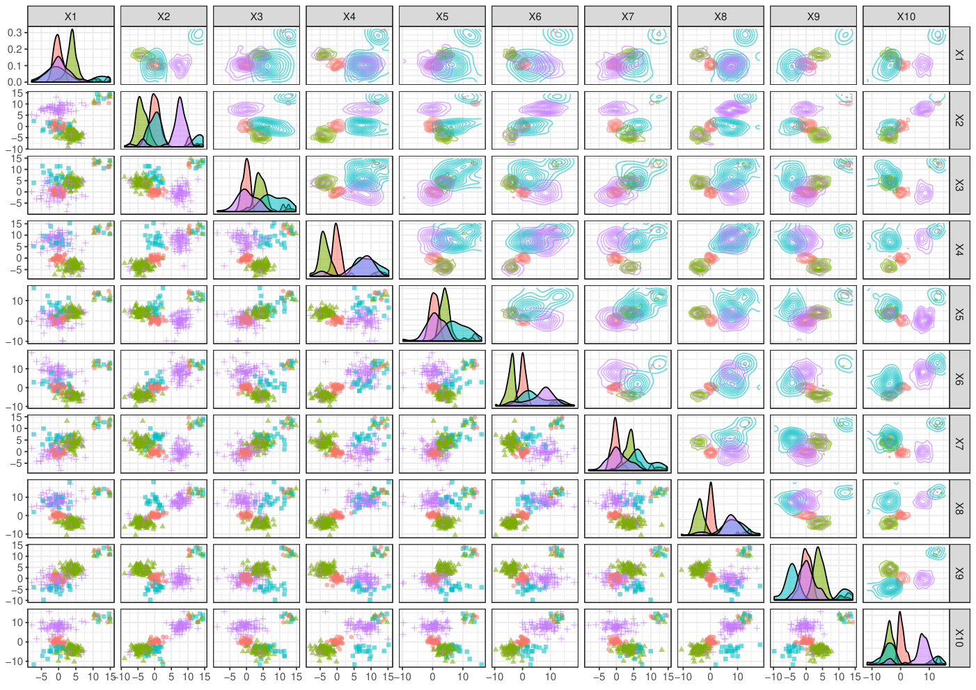
A generalized pairs plot of contaminated labelled units under the afore-described Simulation Setup is reported in Figure 7.
Appendix C
This final Section presents feasible and computationally efficient algorithms for enforcing the eigenvalue-ratio constraint according to the different patterned models in Table 1. At the th iteration of the M step, the goal is to update the estimates for the variance-covariance matrices , such that,
| (33) |
where indicates the diagonal entries of matrix . Denote with the estimates for the variance covariance matrices obtained following Bensmail and Celeux 1996 without enforcing the eigenvalues-ratio restriction in (33). Lastly, denote with the matrix of eigenvalues for , with diagonal entries , .
Constrained maximization for VII, VVI and VVV models
- 1.
Compute applying the optimal truncation operator defined in Fritz et al. 2013 to , under condition (33)
- 2.
Set , ,
Constrained maximization for VVE model
- 1.
Compute applying the optimal truncation operator defined in Fritz et al. 2013 to , under condition (33)
- 2.
Given , compute the common principal components via, for example, a majorization-minimization (MM) algorithm (Browne and McNicholas 2014)
- 3.
Set , ,
Constrained maximization for EVI, EVV models
- 1.
Compute applying the optimal truncation operator defined in Fritz et al. 2013 to , under condition (33)
- 2.
Compute constraining such that . That is, constraining to be equal across groups (Maronna and Jacovkis 1974; Gallegos 2002). Details are given in Section 3.2 of Fritz et al. 2012
- 3.
Iterate until (33) is satisfied
- 4.
Set , ,
Constrained maximization for EVE model
- 1.
Compute applying the optimal truncation operator defined in Fritz et al. 2013 to , under condition (33)
- 2.
Compute constraining such that . Details are given in Section 3.2 of Fritz et al. 2012
- 3.
Iterate until (33) is satisfied
- 4.
Given , compute the common principal components via, for example, a majorization-minimization (MM) algorithm (Browne and McNicholas 2014)
- 5.
Set , ,
Constrained maximization for VEI, VEV models
- 1.
Set
- 2.
Set ,
- 3.
Compute applying the optimal truncation operator defined in Fritz et al. 2013 to , under condition (33)
- 4.
Compute
- 5.
Compute
- 6.
Set
- 7.
Iterate until (33) is satisfied
- 8.
Set , ,
Constrained maximization for VEE model
- 1.
Set
- 2.
Set ,
- 3.
Compute applying the optimal truncation operator defined in Fritz et al. 2013 to , under condition (33)
- 4.
Compute
- 5.
Compute
- 6.
Set
- 7.
Iterate until (33) is satisfied
- 8.
Considering the spectral decomposition for , set , ,
References
- Aitken (1926) Aitken AC (1926) A series formula for the roots of algebraic and transcendental equations. Proceedings of the Royal Society of Edinburgh 45(01):14–22
- Alimentarius (2001) Alimentarius C (2001) Revised codex standard for honey. Codex stan 12:1982
- Banfield and Raftery (1993) Banfield JD, Raftery AE (1993) Model-based Gaussian and non-Gaussian clustering. Biometrics 49(3):803
- Bensmail and Celeux (1996) Bensmail H, Celeux G (1996) Regularized Gaussian discriminant analysis through eigenvalue decomposition. Journal of the American Statistical Association 91(436):1743–1748
- Bohning et al. (1994) Bohning D, Dietz E, Schaub R, Schlattmann P, Lindsay BG (1994) The distribution of the likelihood ratio for mixtures of densities from the one-parameter exponential family. Ann Inst Statist Math 46(2):373–388
- Bouveyron and Girard (2009) Bouveyron C, Girard S (2009) Robust supervised classification with mixture models: Learning from data with uncertain labels. Pattern Recognition 42(11):2649–2658
- Browne and McNicholas (2014) Browne RP, McNicholas PD (2014) Estimating common principal components in high dimensions. Adv Data Anal Classif 8:217–226
- Cattell (1966) Cattell RB (1966) The scree test for the number of factors. Multivariate Behavioral Research 1(2):245–276
- Celeux and Govaert (1995) Celeux G, Govaert G (1995) Gaussian parsimonious clustering models. Pattern Recognition 28(5):781–793
- Cerioli et al. (2018) Cerioli A, García-Escudero LA, Mayo-Iscar A, Riani M (2018) Finding the number of normal groups in model-based clustering via constrained likelihoods. Journal of Computational and Graphical Statistics 27(2):404–416
- Cortes and Vapnik (1995) Cortes C, Vapnik V (1995) Support-vector networks. Machine Learning 20(3):273–297
- Cuesta-Albertos et al. (1997) Cuesta-Albertos JA, Gordaliza A, Matrán C (1997) Trimmed k-means: An attempt to robustify quantizers. Annals of Statistics 25(2):553–576
- Dean et al. (2006) Dean N, Murphy TB, Downey G (2006) Using unlabelled data to update classification rules with applications in food authenticity studies. Journal of the Royal Statistical Society Series C: Applied Statistics 55(1):1–14
- Dempster et al. (1977) Dempster A, N Laird, Rubin D (1977) Maximum likelihood from incomplete data via the EM algorithm. Journal of the Royal Statistical Society 39(1):1–38
- Dotto and Farcomeni (2019) Dotto F, Farcomeni A (2019) Robust inference for parsimonious model-based clustering. Journal of Statistical Computation and Simulation 89(3):414–442
- Dotto et al. (2018) Dotto F, Farcomeni A, García-Escudero LA, Mayo-Iscar A (2018) A reweighting approach to robust clustering. Statistics and Computing 28(2):477–493
- Downey (1996) Downey G (1996) Authentication of food and food ingredients by near infrared spectroscopy. Journal of Near Infrared Spectroscopy 4(1):47
- Fop et al. (2016) Fop M, Murphy TB, Raftery AE (2016) mclust 5: Clustering, Classification and Density Estimation Using Gaussian Finite Mixture Models. The R Journal XX(August):1–29
- Fraley and Raftery (2002) Fraley C, Raftery AE (2002) Model-based clustering, discriminant analysis, and density estimation. Journal of the American Statistical Association 97(458):611–631
- Freund and Schapire (1997) Freund Y, Schapire RE (1997) A Decision-Theoretic Generalization of On-Line Learning and an Application to Boosting. Journal of Computer and System Sciences 55(1):119–139
- Fritz et al. (2012) Fritz H, García-Escudero LA, Mayo-Iscar A (2012) tclust : An R Package for a Trimming Approach to Cluster Analysis. Journal of Statistical Software 47(12):1–26
- Fritz et al. (2013) Fritz H, García-Escudero LA, Mayo-Iscar A (2013) A fast algorithm for robust constrained clustering. Computational Statistics and Data Analysis 61:124–136
- Gallegos (2002) Gallegos MT (2002) Maximum likelihood clustering with outliers. In: Classification, Clustering, and Data Analysis, Springer, pp 247–255
- García-Escudero et al. (2008) García-Escudero LA, Gordaliza A, Matrán C, Mayo-Iscar A (2008) A general trimming approach to robust cluster Analysis. The Annals of Statistics 36(3):1324–1345
- García-Escudero et al. (2010) García-Escudero LA, Gordaliza A, Matrán C, Mayo-Iscar A (2010) A review of robust clustering methods. Advances in Data Analysis and Classification 4(2-3):89–109
- García-Escudero et al. (2011) García-Escudero LA, Gordaliza A, Matrán C, Mayo-Iscar A (2011) Exploring the number of groups in robust model-based clustering. Statistics and Computing 21(4):585–599
- García-Escudero et al. (2014) García-Escudero LA, Gordaliza A, Mayo-Iscar A (2014) A constrained robust proposal for mixture modeling avoiding spurious solutions. Advances in Data Analysis and Classification 8(1):27–43
- García-Escudero et al. (2015) García-Escudero LA, Gordaliza A, Matrán C, Mayo-Iscar A (2015) Avoiding spurious local maximizers in mixture modeling. Statistics and Computing 25(3):619–633
- García-Escudero et al. (2016) García-Escudero LA, Gordaliza A, Greselin F, Ingrassia S, Mayo-Iscar A (2016) The joint role of trimming and constraints in robust estimation for mixtures of Gaussian factor analyzers. Computational Statistics & Data Analysis 99:131–147
- García-Escudero et al. (2017) García-Escudero LA, Gordaliza A, Greselin F, Ingrassia S, Mayo-Iscar A (2017) Eigenvalues and constraints in mixture modeling: geometric and computational issues. Advances in Data Analysis and Classification pp 1–31
- Gordaliza (1991a) Gordaliza A (1991a) Best approximations to random variables based on trimming procedures. Journal of Approximation Theory 64(2):162–180
- Gordaliza (1991b) Gordaliza A (1991b) On the breakdown point of multivariate location estimators based on trimming procedures. Statistics & Probability Letters 11(5):387–394
- Hastie and Tibshirani (1996) Hastie T, Tibshirani R (1996) Discriminant analysis by Gaussian mixtures. Journal of the Royal Statistical Society Series B (Methodological) 58(1):155–176
- Hawkins and McLachlan (1997) Hawkins DM, McLachlan GJ (1997) High-breakdown linear discriminant analysis. Journal of the American Statistical Association 92(437):136
- Hickey (1996) Hickey RJ (1996) Noise modelling and evaluating learning from examples. Artificial Intelligence 82(1-2):157–179
- Hubert et al. (2018) Hubert M, Debruyne M, Rousseeuw PJ (2018) Minimum covariance determinant and extensions. Wiley Interdisciplinary Reviews: Computational Statistics 10(3):1–11
- Ingrassia (2004) Ingrassia S (2004) A likelihood-based constrained algorithm for multivariate normal mixture models. Statistical Methods and Applications 13(2):151–166
- Kelly et al. (2006) Kelly JD, Petisco C, Downey G (2006) Application of Fourier transform midinfrared spectroscopy to the discrimination between Irish artisanal honey and such honey adulterated with various sugar syrups. Journal of Agricultural and Food Chemistry 54(17):6166–6171
- Mardia et al. (1979) Mardia KV, Kent JT, Bibby JM (1979) Multivariate analysis. Academic Press London; New York
- Maronna and Jacovkis (1974) Maronna R, Jacovkis PM (1974) Multivariate clustering procedures with variable metrics. Biometrics 30(3):499
- McLachlan (1992) McLachlan GJ (1992) Discriminant analysis and statistical pattern recognition, Wiley Series in Probability and Statistics, vol 544. John Wiley & Sons, Inc., Hoboken, NJ, USA
- McLachlan and Krishnan (2008) McLachlan GJ, Krishnan T (2008) The EM Algorithm and Extensions, Wiley Series in Probability and Statistics, vol 54. John Wiley & Sons, Inc., Hoboken, NJ, USA
- McLachlan and Peel (1998) McLachlan GJ, Peel D (1998) Robust cluster analysis via mixtures of multivariate t-distributions. pp 658–666
- McNicholas (2016) McNicholas PD (2016) Mixture Model-Based Classification. Chapman and Hall/CRC
- Menardi (2011) Menardi G (2011) Density-based Silhouette diagnostics for clustering methods. Statistics and Computing 21(3):295–308
- Neykov et al. (2007) Neykov N, Filzmoser P, Dimova R, Neytchev P (2007) Robust fitting of mixtures using the trimmed likelihood estimator. Computational Statistics & Data Analysis 52(1):299–308
- Peel and McLachlan (2000) Peel D, McLachlan GJ (2000) Robust mixture modelling using the t distribution. Statistics and Computing 10(4):339–348
- Prati et al. (2018) Prati RC, Luengo J, Herrera F (2018) Emerging topics and challenges of learning from noisy data in nonstandard classification: a survey beyond binary class noise. Knowledge and Information Systems pp 1–35
- R Core Team (2018) R Core Team (2018) R: A Language and Environment for Statistical Computing
- Rousseeuw and Driessen (1999) Rousseeuw PJ, Driessen KV (1999) A fast algorithm for the minimum covariance determinant estimator. Technometrics 41(3):212–223
- Russell et al. (2014) Russell N, Cribbin L, Murphy TB (2014) upclass: An R Package for updating model-based classification rules. Cran R-Project Org
- Schwarz (1978) Schwarz G (1978) Estimating the dimension of a model. The Annals of Statistics 6(2):461–464
- Thomson (1939) Thomson G (1939) The factorial analysis of human ability. British Journal of Educational Psychology 9(2):188–195
- Vanden Branden and Hubert (2005) Vanden Branden K, Hubert M (2005) Robust classification in high dimensions based on the SIMCA Method. Chemometrics and Intelligent Laboratory Systems 79(1-2):10–21
- Wu (1995) Wu X (1995) Knowledge acquisition from databases. Intellect books, Westport, CT, USA
- Zhu and Wu (2004) Zhu X, Wu X (2004) Class noise vs. attribute noise: A quantitative study. Artificial Intelligence Review 22(3):177–210