Practical Valid Inferences for the Two-Sample Binomial Problem
Abstract
Our interest is whether two binomial parameters differ, which parameter is larger, and by how much. This apparently simple problem was addressed by Fisher in the 1930’s, and has been the subject of many review papers since then. Yet there continues to be new work on this issue and no consensus solution. Previous reviews have focused primarily on testing and the properties of validity and power, or primarily on confidence intervals, their coverage, and expected length. Here we evaluate both. For example, we consider whether a p-value and its matching confidence interval are compatible, meaning that the p-value rejects at level if and only if the confidence interval excludes all null parameter values. For focus, we only examine non-asymptotic inferences, so that most of the p-values and confidence intervals are valid (i.e., exact) by construction. Within this focus, we review different methods emphasizing many of the properties and interpretational aspects we desire from applied frequentist inference: validity, accuracy, good power, equivariance, compatibility, coherence, and parameterization and direction of effect. We show that no one method can meet all the desirable properties and give recommendations based on which properties are given more importance.
Keywords:
Unconditional exact test,keywords
[class=MSC]keywords
and
1 Introduction
Suppose we observe two independent binomial variates with parameters and . Two questions are: are and equal? and how much larger is one parameter than the other? To answer these two questions, the frequentist typically presents an estimate of an effect, a confidence interval (CI) on that effect, and a p-value to test that there is no effect. Surprisingly, there is no consensus method for testing and creating confidence intervals for this problem. New methods continue to be developed for this problem [38, 57, 58, 21, 27, see e.g.,]. Many review papers focus on testing alone [40, 48, see], or confidence intervals alone [46, 53, 17, see]. Here we focus on both.
We limit the scope of this paper by considering only frequentist approaches (so Bayesian methods are not covered), and by not considering asymptotic methods or other approximations. Many review papers or books [46, 40, 17, 47, see e.g.,] cover and compare many of those approximations. Sometimes those approximations are closed-form expressions and can be useful for deriving simple sample size formulas or when the test is applied many times such as in genomics. But often the approximations are unnecessary with modern computers. Non-asymptotic methods are often called exact, but in this paper we reserve the term exact for non-asymptotic methods that are valid, meaning tests that control the type I error rate, and confidence intervals that cover the parameter with at least the nominal value. See Section 2.2 for further discussion of the term exact. A class of important non-asymptotic tests that are not valid are mid-p methods (Section 9), which are sometimes called quasi-exact [29] and are included in our review because, for confidence intervals, sometimes we want average coverage close to the nominal value instead of guaranteed coverage that on average is conservative.
Here is an outline of our paper. Section 2 begins by contrasting the two-sample binomial problem with the two-sample difference in normal distributions with the same variance, in which there is an accepted solution: the two-sample t-test. This allows us to define inferential properties of interest as well as highlight why there is no single accepted solution to the two-sample binomial problem. Newcombe [47] takes a similar approach. Section 3 discusses the choice of effect measure (e.g., difference in binomial parameters, ratio of parameters, or odds ratio of parameters). Section 4 defines a frequentist triple as a parameter estimator, an associated confidence interval procedure, and a p-value function. We then formally discuss some properties of triples, such as whether the confidence interval and p-value match and are compatible, and whether directional inferences may be made from the triple. The idea of matched triples is discussed in Hirji [28, p. 77] in a less formal way as a “unified report”. Our review says very little about parameter estimators, and mostly focuses on properties of p-values and confidence intervals and the compatibility of p-values with confidence intervals. Our discussion of directional inferences is motivated from the three decision rule of Neyman [26, see e.g.,]. We describe methods for defining valid one-sided decision rules in Sections 5 (unconditional methods) and 6 (conditional methods), including the associated p-values and confidence intervals. Much of Sections 5 and 6 was thoroughly reviewed in [48] but is included in this paper for completeness; however, Section 5.3 presents some new ideas on informativeness of ordering functions. Section 7 reviews the melded confidence intervals of Fay, Proschan and Brittain 2015 which are compatible with the one-sided conditional method (i.e., Fisher’s exact test) p-values. Section 8 discusses non-central confidence intervals and associated tests, with a new focus on the relationship of these intervals to directional inferences. Section 9 discusses mid-p methods, which are non-asymptotic methods that relax the validity assumption in order to achieve better accuracy. Section 10 discusses the computational aspects of various methods. Section 11 discusses power and efficiency of methods, including some new calculations. Section 12 presents recommendations. Briefly, we recommend using exact central confidence intervals (those with equal error bounds on both sides) because it is better for directional inferences. For fast calculations, use exact conditional tests with compatible confidence intervals, but for more power consider exact unconditional test using the version that orders by the one-sided mid-p Fisher’s exact p-values. If validity is not vital, use mid-p values on the exact conditional test, which are often a good approximation to the exact unconditional tests.
2 Overview: Failure of Normal Intuition
2.1 Frequentist Inferences
We define a frequentist triple (or just a triple) as an estimator of a parameter of interest, a confidence interval, and a p-value function. This approach allows us to compare different triples by examining not just properties of each component (i.e., comparing powers of different p-value functions or expected lengths of different confidence intervals), but also to examine properties of the triples as a whole. For example, within a triple, we examine inferential agreement between the p-value function and confidence interval procedure. Additionally, we examine what directional inferential statements we can make from the triple, such as whether is significantly larger than , and at what significance level.
Although in some different statistical settings (e.g., two-sample normal problem) the standard triple will automatically give inferential agreement between p-values and confidence intervals as well as automatically give directional inferential statements, in the two-sample binomial problem those inferential properties are not automatic. Thus, before discussing the binomial problem, we review the two-sample problem with normally distributed responses with the same variance. We consider the latter problem first, because there is some consensus that one triple (the difference in means, and the confidence interval and p-value associated with the t-test) is appropriate for this problem. In the normal case, this t-test triple meets some regularity properties that lead to inferences that are intuitive and easy to understand. Because these properties form the basis for a certain statistical intuition about how frequentist inferences ought to be, and because the example uses normal distributional assumptions, we call these properties the “normal intuition”. We show later how the normal intuition breaks down for the two-sample binomial problem, although many of the properties may approximately hold for large samples.
2.2 Background and Notation
Consider a general frequentist problem, where we observe data, , and denote its random variable as . Assume some probability model for that depends on a parameter vector , but we are interested in a function of that returns a scalar, . We partition the possible values of into two sets, the null hypothesis space, , and the alternative hypothesis space, .
In this paper, we consider only three classes of partitions, where the null and alternative space is defined by , and separated by a value on the boundary between the null and alternative hypothesis spaces. The first of these three classes are two-sided hypotheses,
which can be equivalently written as
The other two classes are the one-sided hypotheses,
| Alternative is Less | Alternative is Greater | |||
Let be a p-value associated with the null hypothesis space, . Typically, we assume a class of hypotheses and write (with a slight abuse of notation) as a p-value associated with the null hypothesis indexed by . We reject the null hypothesis at level if . Following Berger and Boos 1994, we define a p-value procedure as valid if
for all and all . (Ripamonti, et al [48] call a valid p-value procedure a guaranteed p-value.) The term exact is often used to describe tests that give valid p-values, but be aware that the term ‘exact’ is used in at least 4 different ways in the literature: (i) methods not based on asymptotic or other approximations [see 28, p.450], (ii) valid methods [29, 40, 21, see], (iii) methods where the size is equal to the significance level (only possible with randomized tests for discrete data) [16], or (iv) methods where the p-values are the smallest p-values among a class of valid p-values [48, equation 2.5], specifically, p-value procedures such that
| (2.1) |
In this review, we use the term exact only in the sense of (ii).
Following Röhmel 2005, we define a p-value procedure as coherent if for every , if .
For the classes of hypotheses above, we can invert the p-value function to get its associated confidence region,
| (2.2) |
We define a confidence region as valid if it is guaranteed to have at least nominal coverage for every (and hence every ); in other words,
This paper considers non-asymptotic methods, and all are valid except the mid-p methods described in Section 9.
2.3 Standard Frequentist Inference: Normal Intuition
Consider the two-sample problem, where the th group has independent and normally distributed responses, with mean and variance , for . Let , and suppose we are interested in . The t-test is valid for testing the null that and it is the uniformly most powerful (UMP) unbiased test [37, p. 160]. UMP unbiasedness means that among the class of unbiased tests (i.e., tests for which power for each parameter value in the alternative space is at least as large as the power for every parameter value in the null space), the t-test is the most powerful test for each .
We study this case first to define “normal intuition” about frequentist inferences. This normal intuition is a series of properties, that if they are not met, conflict with many statisticians’ intuitive feeling of how p-values and confidence regions ought to work. Here are those properties met by the triple: difference in sample means, ; the two-sided p-value from the t-test, ; and the confidence interval on associated with that p-value, .
- Reproducibility:
-
Application of the method by two independent statisticians to the same data always gives the same results (as opposed to randomized tests).
- Confidence region is an interval:
-
The confidence region created from through equation 2.2 is an interval, meaning it can be written as .
- Compatible Inferences:
-
if and only if the confidence interval does not contain .
- Accuracy (of coverage):
-
Taken over repeated applications, the probability that the confidence interval procedure includes is equal to for all values of such that .
- Centrality (of CI):
-
The CI is a central one, meaning and .
- One-sided p-value from Two-sided p-value:
-
Half of the two-sided p-value can be interpreted as a one-sided p-value in the apparent direction of the effect. For example, if then we can reject at level .
- Directional Coherence (of p-value):
-
Call a two-sided p-value function directionally coherent if the p-values are decreasing as gets farther from . In other words, directionally coherent two-sided p-values have when either or . A two-sided p-value with this property can be interpreted as a coherent one-sided p-value in the appropriate direction. For example, if then we can reject at level . (And for the t-test p-value, we can also reject at a level of .)
- Monotonicity (of power):
-
Under the alternative hypothesis, power increases as the sample size increases.
- Nestedness (of CIs):
-
If , then the confidence interval, , would contain the one, ; in other words, .
2.4 Two-Sample Binomial: Failure of Normal Intuition
Now we turn to the two-sample binomial problem, where and independently . Here the parameter of interest is typically one of three functions of : the difference (), the ratio (), or the odds ratio (). In this problem, the inferential methods do not necessarily follow the properties that we would expect from normal intuition. We list several examples using several different valid tests, valid confidence intervals, or triples.
- Failure of Reproducibility:
-
The uniformly most powerful unbiased (UMPU) test of versus is a randomized version of a one-sided Fisher’s exact test [37, 23, see e.g.,]. Testing this hypothesis at the one-sided level for the data and , the UMPU test rejects 70.3% of the time. So, provided they are not using the same pseudo-random number generator, there is a 41.7% chance that two researchers applying the UMPU test to those data will have different accept/reject decisions.
- Associated confidence region not an interval:
-
There are two versions of the two-sided Fisher’s exact test and the most common is the Fisher-Irwin test (default in current versions of SAS [version 9.4] and R [version 4.0.4], see Section 8 for definition). The test was designed to test , but it can be generalized to test other null hypotheses. Consider the data and [see 19, Supplement, Section 3.1]. The two-sided p-value for testing is , which rejects the null hypothesis at the level. If we slightly change the null and test , we get , and we fail to reject. But counter-intuitively, if we change the null the other way and test , we also fail to reject, . So if we create the confidence region by inverting the p-value procedure, this region is not contiguous,
and includes values of both larger and smaller than . The cause of this behaviour is the lack of unimodality of the p-value function; see Figure 1.

Figure 1: Two-sided Fisher’s exact test (Fisher-Irwin version) p-values by for and . Right panel is an enlargement of part of the left panel. Reference line is . - Incompatible inferences:
-
If the confidence region is not an interval, we can create a valid CI by using the interval that covers the whole confidence region. But this will not give compatible inferences with the p-value function. Returning to the Fisher’s exact test confidence region example, we can create a 95% confidence interval by “filling in the hole” as to create the matching confidence interval [6, see Section 4.1 or Ref.]. In this case, the two-sided p-value rejects the null that at the level, but the matching 95% confidence interval includes . This issue is different from the incompatible inferences that often occur by using different methods to calculate p-values and confidence intervals, which can be quite prevalent in this application. For example, the default for R (fisher.test in base R, version 4.0.4) and SAS (exact option in Proc Freq, version 9.4) uses the Fisher-Irwin two-sided p-value, but calculates the two-sided confidence interval on by inverting two one-sided Fisher exact p-values [19, 20, see e.g.,].
- Imperfect Accuracy of Coverage:
-
Because of discreteness, the valid confidence interval must have coverage larger than the nominal level for some values of , in order to ensure validity for all values of . Remember, the term “exact” is often used to mean valid (see Section 2.2), so an “exact” confidence interval may have coverage greater than the nominal level and not, as the term might imply, have coverage exactly equal to the nominal level. Section 9 discusses relaxing the requirement of validity in order to have coverage closer to the nominal level “on average”, slightly greater than nominal for some parameter values and slightly less for others.
- Non-Centrality of Confidence Interval:
-
Although central CIs for the binomial problem are important, much has been written on non-central intervals. Agresti and Min 2001 showed that inverting certain two-sided tests, produces shorter confidence intervals than central ones. For the difference in proportions, this strategy often uses an unconditional exact (i.e., valid) version of a two-sided score test [17, see]. For and , the difference in proportions is with 95% confidence interval and the associated two-sided exact p-value for testing is . Because the 95% confidence interval is based on inverting a two-sided test, we cannot use as a one-sided p-value to show that at the level. In fact, to ensure validity, we can only use the two-sided p-value as an upper bound on that one-sided p-value.
- Non-monotonicity of power:
-
Continuing with the previous example ( and using the unconditional exact two-sided score test), if we add one more observation to group 2 the two-sided p-value increases regardless of whether the extra observation is a failure (giving and ), or success (giving and ) [56, this example comes from]. Thus, it is not surprising that the power to reject at the two-sided level when and is higher for (power= 61.9%) than for (power=53.7%). Power non-monotonicity can also exist for common one-sided tests. Using a one-sided Fisher’s exact test (to reject ) at the level, when the only way to reject is the most extreme case, and , and the power to reject is . When and then still the only way to reject at the level is the most extreme case, and , and the power is . Then, for all and , and the power with the larger sample size is smaller. A similar decrease in power occurs by instead adding one to the other group: and .
- Non-nested Confidence Intervals:
-
Wang 2010 proposed a method for constructing the smallest one-sided confidence interval for the difference of two proportions. Consider and . The lower one-sided 95% interval on the difference, , is , but the 96% interval by the same method is . See Figure 2 and Section 5.5.

Figure 2: Thick gray lines are lower limits for the smallest one-sided confidence limits for from Wang 2010 for and . Solid black lines show one-sided 95% limit of , while dotted black lines show one-sided 96% limit of . - Non-Coherence:
-
For testing for non-inferiority on a difference in proportions, Chan and Zhang 1999 recommend the exact unconditional test based on the score test. Röhmel 2005 gives the following illustrative example: the proportion of failures on control is and on new treatment is , with the failure rate slightly lower on new treatment, . If we want to show that the p-value is , but if we want to show an even less stringent margin, the p-value non-intuitively increases to (see Figure 3 and Section 5.6).
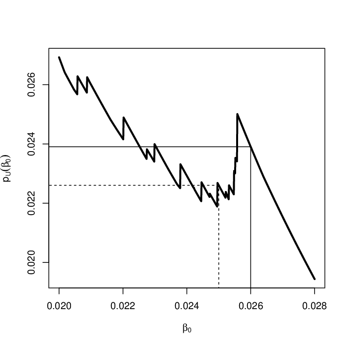
Figure 3: One-sided exact unconditional p-value using the score statistic ordering, . Virtual data example from Röhmel 2005: and . Thick black line is the p-value function. Thin black lines depict the test of the null and dotted lines depict the test of the null .
For the two-sample binomial problem, many attempts to increase power or get the smallest expected length CI result in violations of some of these “normal intuition” properties.
3 Choosing the Effect Measure
Choosing the effect measure is dependent on the application, so we examine a real application to discuss the issues. Coulibaly et al. 2009 studied a parasite called Mansonella perstans that infects people in parts of Africa. The usual drugs that kill other similar parasites had not been working on killing M. perstans. Coulibaly et al. 2009 realized that in this case there was a symbiotic bacteria, Wolbachia, that helped the M. perstans live. They suspected that if they gave a common antibiotic, doxycycline, to kill the bacteria, it may in fact help cure the patient of M. perstans. Patients were randomized to the treatment group (doxycycline) or the control group (no treatment). There are issues of missing data that we ignore for simplicity. At 12 months, out of subjects who received doxycycline and out of had cleared the M. perstans from their blood. There are several reasonable choices for how to measure the effect: the difference in clearance rates, the ratio of clearance rates, the ratio of failure probabilities, and the odds ratio of clearance rates. Although the choice is often dominated by what is most natural to the intended audience, there are some statistical issues related to this choice.
Without loss of generality, consider effect measures that measure how much larger is than . The opposite effect can be measured by switching group labels. But we could also simultaneously switch group labels and switch the response and failure labels. If the effect remains the same after this double switching, we say that the measure has symmetry equivariance. The measures and have symmetry equivariance; however, does not have it, as we demonstrate with the example. Let and . An estimate of the rate ratio for success (cleared parasites at 12 months) is . The rate ratio is often called the relative risk, but in this case the “risk” is the risk of getting cured. A different expression of the same data measures the ratio of the rates of failures (those still having detectable parasites at 12 months). Let and . Then an estimate of the relative risk of failure is . In this latter case the control group looks about 29 times worse than the treatment group, while if we look at the rate ratios for success, the treatment group looks only about 6 times better than the control group. So how many times better treatment is than control depends on which way we measure risk. This is a violation of symmetry equivariance. Despite this, the rate ratio is often used because it is easy to understand [14, see e.g.,], or because it has become the parameter of choice within a field, so that its use facilitates comparisons between studies.
The difference has symmetry equivariance. If we measured the difference in rates of disease rather than the difference in rates of cure we get exactly the negative difference as we might expect. Similar to the relative risk, the difference is often used because it is easy to understand. Additionally, the sample difference in rates is always defined, unlike the ratio which is undefined when .
Figure 4 plots the three statistics using and with . The plots go from dark blue ( is larger) to white () to dark red ( is larger), with black denoting indeterminate. Because of the indeterminate black areas, the ordering of the sample space for the ratio and odds ratio is not straightforward (see Section 5.3). The ordering of the measures on the parameters themselves would give a continuous version of Figure 4, and the black regions would reduce to points at or . The bottom panels show the lack of symmetry equivariance for . Comparing the panel for with the two different ratio panels, we see that the lower left hand corner of the panel is similar to the lower left hand corner of . For small , is a good approximation to . Similarly for both values close to , is a good approximation of (right bottom panel).

The odds ratio is the most complicated of the three measures, but it has some nice properties. It is very important for the case-control design used to study rare diseases, because the odds ratio of disease given exposure is equal to the odds ratio of exposure given disease [8, see]. Also for performing regression on binary observations, logistic regression allows linear predictors to be used to model the log odds, and effects of binary covariates can be expressed as odds ratios. An advantage of the odds ratio for the two-sample binomial case is that by conditioning on the total number of successes in both groups, the probability distribution reduces to a noncentral hypergeometric distribution which is a function of . This is discussed more in Section 6.
4 Properties of Frequentist Triples
4.1 Defining a Matched Triple
Once we choose an effect measure, we choose an appropriate triple (an estimator, confidence interval, and p-value function) for inferences. We will not specify the estimator except to require that it is within the confidence interval. We focus mostly on choosing the CI and p-value function. Except in Section 9, we only consider triples that are valid (i.e., the CI and p-value are both valid) and reproducible. Because we require reproducibility, the triple based on the UMP unbiased (and randomized) test is not allowed. We focus on triples where the p-value function and the confidence interval are derived from the same procedure. We call this a matched triple.
Here is a precise definition of a matched triple. If we start with , an associated confidence region is given by equation 2.2, and the matching CI is smallest interval that contains that confidence region. In other words, if the confidence region has holes in it, then those holes are “filled in”. On the other hand, if we start with , then the matching p-value function is the smallest such that is outside for all .
4.2 Implications of Compatible Inferences
Theorem 4.1.
Consider a valid, reproducible, and matched triple. The triple has compatible inferences
- 1.
if and only if the CI is equal to the confidence region associated with the p-value, and
- 2.
only if the CI is nested, and
- 3.
only if the the p-value function is coherent (for one-sided p-values), or directionally coherent (for two-sided p-values).
The formal proof of the theorem is in Appendix A. The theorem says we must have nested CIs and coherent p-values in order to have compatible inferences. These ideas are best understood graphically. Figure 1 shows lack of directional coherence; for every there is only one p-value, and the two-sided p-value function is not unimodal (i.e., as increases, the p-value function does not increase to the global maximum, then decrease after that; see the right panel). Similarly, Figure 3 shows lack of coherence. Figure 2 shows non-nestedness; for every there is only one lower limit, and the lower limit is not a monotonic function of the level.
4.3 Directional Inferences
Typically, a researcher who finds a significant difference from the two-sided p-value suggesting that is almost always interested in interpreting the result in terms of whether or . In other words, the two-sided hypothesis test is often treated as a three-decision rule: (1) fail to reject , (2) reject and conclude , or (3) reject and conclude . If the two-sided p-value has directional coherence, then if we reject at level , we can additionally reject at level either (if ) or (if ).
Consider comparing two triples that both have compatible inferences, one with a central CI, and one with a non-central CI. For the non-central triple (i.e., the one with the non-central CI) the associated two-sided hypothesis test may be slightly more powerful, but if the non-central triple is applied also to a subsequent one-sided hypothesis (as in the three decision rule), it can be quite a bit less powerful than the central one. To see this, start with a nested central CI, say , and pair it with its matching two-sided p-value, say . By Theorem 4.1, this means that whenever the CI excludes then , and we can reject at level . After rejecting the two-sided hypothesis at level , we can reject one of the one-sided hypotheses at level ; if we reject , while if we reject . A non-central CI does not allow one-sided rejections at the level. Freedman 2008 discusses this issue in terms of clinical trials, and, using these arguments as well as some Bayesian motivation, [26] recommends performing two one-sided tests at the level, which is another way of describing the use of central CI methods for three decision rules.
In summary, if we desire directional inferences, and we want to compare the power to detect a one-sided effect in a fair way (i.e., both methods bound the one-sided type I error rates of the three decision rule at the same level), then we need to compare a method with a two-sided p-value and its matching non-central CI, with a pair of one-sided p-values and its matching central CI. This means that when comparing expected lengths of CIs, if directionality of effect is important, we should compare the expected length of a non-central CI with the expected length of a central CI. Because directionality is usually important, our default recommendation is to use central confidence intervals and perform three-sided inferences as described above.
5 Methods for Creating One-Sided Exact Unconditional Testing Procedures
5.1 Basic Procedure for Defining p-values
Suppose larger values of are better. We want to know if treatment 2 is better than treatment 1 (), and by how much. Let be a function of the data, where larger values of indicate that treatment 2 is better than treatment 1, and is defined for all possible values of . For example, a simple is the difference in observed proportions (see Figure 4 upper left). For this section and the next (Section 5.2), we require that is a function of only. Later in Section 5.5, may depend on , and in Section 5.6, may depend on . Barnard 1947 outlined convexity conditions which ensure that larger values of suggest treatment 2 is better. Barnard’s convexity (BC) conditions are:
| if | then | (5.1) | |||
| and | |||||
| if | then |
Many choices for satisfy the BC conditions. For example, meets the BC conditions.
Once we have decided on the ordering function, , we can create valid unconditional one-sided p-values: for testing the null (defined as ) and for testing () using
| (5.2) | |||||
| and | |||||
These p-values are valid since
where for and for . The p-values are also ‘exact’ by the terminology of [48] (see equation 2.1, or Theorem 1 of [38]). Thus, any other valid p-values with ordering based on are inadmissible (that is, they have values that are never less than the valid unconditional p-values and are greater for at least one ) [38, Theorem 2].
These valid one-sided p-values can be inverted to create two one-sided confidence limits using
| (5.7) | |||||
| and | |||||
where for and for or . A central confidence interval is the union of the one-sided ones, , and a central p-value is . These confidence limits are called exact unconditional [44, see e.g.,] or Buehler confidence limits [39, see]. Lloyd and Kabaila 2003 and Wang 2010 show two results about these one-sided intervals. First, the lower and upper one-sided confidence limits retain a logical ordering analogous to Barnard’s convexity conditions. Specifically, , where is the class of valid central confidence intervals such that if then and . Second, calculated in this manner is the smallest confidence interval within . In other words, any other valid central confidence interval in must have and for all .
Barnard 1947 proposed the two-sided CSM test (we discuss the name later). We define the CSM test more generally using an ordering method which may be used for one or two-sided tests and confidence intervals, and we begin with the one-sided versions. Briefly, Barndard’s CSM one-sided ordering starts from the most extreme point and incrementally adds more points to the order such that (1) the new point(s) and all previous points meet the BC conditions, and (2) the new point(s) have the lowest one-sided p-value among the possible new points that meet the BC conditions. Details are in Appendix B. Once the appropriate one-sided CSM ordering function, , is defined, we use the above definitions for the p-values (equation 5.2) and confidence intervals (equation 5.7). The CSM stands for convexity, symmetry, and maximum. Convexity refers to the BC condition that each new point must meet, and maximum refers to the maximization of the null hypothesis space in the definition of the p-value (see sup expression in equations (5.2)). The symmetry condition only applies to the two-sided version of the CSM test, but nevertheless we use “CSM” to describe all versions. The symmetry condition states that whenever a point is added to the order, one must simultaneously add and give it the same value in the ordering (see Appendix B and Section 8 for more discussion of two-sided tests).
In a different paper, Barnard 1945 outlined the general exact unconditional test, and those tests are sometimes referred to as “Barnard’s test” [54, 15, see e.g.,], but we do not use that terminology to avoid confusion with Barnard’s CSM test. Röhmel and Kieser 2013 discussed one-sided exact unconditional tests using Barnard’s CSM p-value ordering, except with breaking more ties to get higher power, an idea discussed in the next section.
Martín Andrés, Sánchez Quevedo and Silva Mato 1998 proposed a good all-purpose ordering, which is to base the ordering on the one-sided mid-pvalue from Fisher’s exact test (see equation 9.1). We explore the power properties of this ordering in Section 11. Alternatively, the ordering can be tailored to a specific application. For example, Gabriel et al. 2018 proposed an ordering to optimize power for certain types of animal experiments where , the parameter for the control group, is expected to be nearly 1.
5.2 Improving Power by Breaking Ties: Refinement of Ordering Functions
One important way to improve the power of some unconditional exact tests based on a function is to break any ties that exist in the ordering function. If is an ordering function with ties, and is an ordering function that gives the same ordering of at all the untied values and additionally breaks some ties, then we say is a refinement of . Then the unconditional exact p-values formed with are always less than or equal to those formed with [see 51, p. 158]. Similarly, one-sided exact unconditional lower confidence limits formed using are always at least as large as the ones formed using [35, 57].
We describe one specific refinement or tie breaking algorithm for the difference in proportions next, which as far as we are aware, has not been specifically described in the literature and has not been available in software (although there are some closely related methods). We can order within each set of tied values using Wald statistics for , i.e., ordering by
where . This leaves the ties for , but otherwise defines points with more precision as more extreme, where extreme is further away from zero. Not all the values with break all the ties. For example, consider the ties at that happen at the values , , , and , for . This method still leaves tied the two pairs of points, and . These remaining ties we argue should remain tied in order for the ordering to retain symmetry equivariance. Note that this suggested ordering is similar, but not equivalent to just ordering the entire sample space by [44, as was studied in].
If we break the ties in this way, then the BC conditions are still met, because only at the boundaries (where the ties are broken according to the BC conditions) do the ties occur at two points and with or . All of the other ties will not have any or so they can be broken in any manner and the overall ordering function, , will meet the BC conditions. This is important for computation (see Section 10). Further, the proposed (tie-breaking on difference in proportions) does not depend on or like some score test based methods (see Sections 5.5 and 5.6) so avoids problems with nesting and coherence.
5.3 Ordering Functions for Ratio and Odds Ratio
Performing exact unconditional tests on or is not straightforward. We consider first since it is simpler. One problem is that could occur with high probability if the true ratio was or if it was as long as both and were very small. So if is designed so that larger values suggest , it is not clear how to define if our interest is in .
Since gives no information about , we must deal with in a special way; set the p-value at to for tests of regardless of the null hypothesis. This means that is placed “deepest” within the null. Following equations 5.2, this implies can be thought of as the largest value when calculating and the smallest value when calculating . A similar issue applies to the odds ratio, except in that case, the point also has no information about .
For clarity, we rewrite equations 5.2 applied to all three parameters. Let denote the set of values with information about . Then if set and to , otherwise let be
and analogously, let be
Since we never reject when , these definitions give valid p-values, and additionally when we do not need to define .
5.4 Other Improvements: E+M and Berger-Boos
Another method to apparently improve the ordering statistic for any efficacy parameter (difference, ratio, or odds ratio) is the estimated and maximized () p-value [38]. In this method, we replace an ordering statistic, , with , where is an estimated p-value when testing (or the negative estimated p-value when testing ). We estimate the p-value by plugging in instead of taking the supremum of under the null, where is the maximum likelihood estimator of . For example, the approximation for in expression 5.2 uses . Then we “maximize” using instead of as the ordering function. That is, we calculate the exact conditional p-value using expression 5.2 by taking the supremum. Lloyd 2008 studied this method and observed that when (the approximate p-value) is used as the ordering statistic, the resulting exact unconditional p-value is generally smaller than the exact unconditional p-value on . The process can be repeated (replace by its approximate p-value), but the additional reduction appears to be minimal.
Berger and Boos 1994 introduced a popular adjustment that tends to reduce exact unconditional p-values. Instead of taking the supremum over the entire null hypotheses parameter space, take the supremum only over , a confidence set of restricted to be in the null space, then add to ensure validity. This is usually done by reexpressing the parameter space as , where is a nuisance parameter, then defining as the intersection of and the set of values with in its confidence interval. A Berger-Boos version of of expression 5.2, uses
This is not optimal, since we may be able to improve it by using as an ordering function. Nevertheless, it usually provides some reduction in p-values [38, see e.g.,].
5.5 Ordering Functions That Depend on Significance Level
Kabaila and Lloyd 2003 showed that for one-sided exact unconditional upper confidence limits, the ordering function, , that maximizes the asymptotic efficiency is an approximate one-sided upper confidence limit itself. A different ordering function is used for the upper and lower limit, and for different confidence levels.
Wang 2010 and Wang and Shan 2015 also proposed an ordering function to give the smallest CI, and the calculation of the ordering function itself is iterative and quite involved, similar to the CSM test of Barnard 1947. The precise definition of the ordering is notationally cumbersome, but the idea is roughly as follows. Consider the lower one-sided limit. Start from the most extreme point . Then add points one at a time, picking the point, , that gives the largest and belongs to the set of closest neighboring points with the already included points, where closest neighbor is defined in terms of the BC conditions. The algorithm ensures that the lower limit function meets the BC conditions. Because each added value is as large as possible, if the resulting ordering function gives the finest partition (there are no ties), then any valid one-sided lower limit that meets the BC conditions and uses for ordering, say , has for all [57, 58, see].
The price for this optimality property is that the ordering function depends on . Different ordering functions arise for different , which can lead to non-nestedness (see Figure 2).
5.6 Ordering Functions That Depend on Hypothesis Space Boundaries
Basing the ordering statistic on a score test can increase power over using simple Wald-type Z statistics [9, see]. Although this increased power has been shown in several simulation studies, it is not clear whether the increase is due to fewer ties for the score test, or from some other difference between the ordering statistics. A problem with the score statistic is that the induced ordering may change based on the , since score statistics use in their calculation, whereas most other test statistics do not include in the calculation. This can produce non-coherence as was shown in Section 2.4 and Figure 3.
6 One-Sided Conditional Exact Tests
Yates 1984 argues that conditioning on the total number of failures is the proper strategy for this problem, and most of the discussants of the paper agreed with this (including Barnard, who first suggested the unconditional approach). One of the main reasons that others had recommended the unconditional approach is an overemphasis on the fixed significance level and the resulting power, which when used leads to more power for unconditional tests because the sample space has more values and hence is less discrete. Yates 1984 argues (in his Section 9) that over reliance on the nominal significance level is not a good reason to prefer the unconditional test, and that p-values should be reported instead of accept/reject decisions. Yates 1984 also argues for conditioning on the total number of events (), because that statistic is approximately ancillary to the effects of interest. Chernoff 2004 quantifies the approximate ancillarity, showing that the absolute amount of information “is quite small unless [ and ] are very far apart”, and the proportion of information in the margins decreases with the sample size. Recent reviews [40, e.g.,] have emphasized power arguments, and we review the choice of test from that perspective in Section 11. Historically, conditional tests have been important because of their much smaller computational burden compared to unconditional tests. The computational burden for unconditional tests has become less important, although for some applications it may be a non-trivial concern (e.g., big data applications with small sample sizes but very many covariates being tested).
For the unconditional one-sided exact method, to calculate p-values we need to take the supremum of the probability that is at least as extreme than the observed over the parameter space (see e.g., equation 5.2). This is a difficult calculation (see Section 10). An alternative method conditions on the sum , and calculates the conditional probability. The resulting conditional distribution is the extended hypergeometric distribution [32] also called Fisher’s noncentral hypergeometric distribution [25], which depends only on . Additionally, because is fixed, we can write the ordering function in terms of only. In fact, the only unique ordering function that makes sense and meets the BC conditions is itself (ordering on will be equivalent). So this simplifies the calculations if the effect measure is . For example, for testing use
| (6.1) | |||||
where the last step follows because the conditional distribution is monotone in [45]. The other conditional one-sided p-value, is calculated similarly except by reversing the inequality. These conditional p-values for testing (or equivalently ) are Fisher’s exact one-sided p-values. We calculate the central confidence intervals on using equation 5.7 except using the conditional exact one-sided intervals instead of the unconditional ones.
Now consider the other measures, and . At the boundary of equality, the one-sided hypotheses are equivalent. For example, the following three null hypotheses give equivalent : (odds ratio) , (ratio) , and (difference) . Analogously for the other one-sided p-value. But for boundaries not representing equality, changes depending on the effect measure. The simplification of the p-value calculation only works for the odds ratio. For example, for the difference in proportions (i.e., ) there is no simplification analogous to equation 6.1. Figure 5 shows that the exact one-sided conditional confidence limit on is not efficient, because the conditional distribution depends on . The upper limit for , say , based on the upper limit for , say , is [see 52, Section 2]
There are better ways to get confidence intervals on and that provide compatible inferences with the one-sided p-values with representing . We show these in the next section.

7 Melded Confidence Intervals
Fay, Proschan and Brittain 2015 developed melded confidence intervals, a general method for creating confidence intervals for the two-sample case, that is closely related to the confidence distribution (CD) approach [59]. Confidence distributions are a frequentist analog to the Bayesian posterior with a non-informative prior. These melded confidence interval give compatible inferences with the central conditional tests.
Before discussing the binomial case, we consider the normal case because it is more straightforward. Consider the difference in means between two normal samples with different variances. Let , , , and be, respectively, the mean, the sample mean, sample size, and unbiased sample variance estimate for group . The two one-sided confidence intervals for the mean in group , are
| and | ||||
with
| (7.1) | |||||
| and | |||||
where is the th quantile of the t-distribution with degrees of freedom. The central confidence interval is the intersection of the two one-sided intervals,
The confidence distribution approach is a way to re-express the confidence interval. Let and be two independent uniform random variables. Let and be the lower and upper confidence distribution random variables for , where the randomness comes from and , while and are treated as constants. From (7.1) and the probability integral transformation, we re-express those random variables as
| and | ||||
where and are independent and distributed with degrees of freedom. Because of the symmetry of the distribution about , and have the same distribution, so in this case the lower and upper confidence distributions are equivalent, and we let be the confidence distribution random variable associated with . In terms of the CD-RV, the confidence interval for is
where is the th quantile of the random variable .
The confidence distribution approach appears to be a confusing and roundabout way to express the confidence interval. The advantage comes when we want a confidence interval for , based on a two-sample problem with independent samples. Then we can write the confidence interval for as
| (7.2) |
which can be estimated with Monte Carlo simulation. Expression 7.2 is equivalent to the Behrens-Fisher confidence interval, and the confidence distribution approach gives a simple way to conceptualize it [21]. The traditional approach calculates the Behrens-Fisher statistic,
and calculates its distribution, which depends on and [36].
For the binomial problem the lower and upper confidence distributions are not equal. Let , for . Let the exact central confidence interval for (i.e., the Clopper-Pearson interval [12]) be
where and are exact one-sided confidence limits, for for . The lower and upper CD random variables for group are and , where are independent uniform random variables. This gives, with expectation , and with expectation , and using limits of parameters going to zero we define as a point mass at and as a point mass at . The lower CD-RV is stochastically smaller than the upper CD-RV. In CD form, the Clopper-Pearson interval is
The melded confidence interval for is
where in order to be conservative for the lower limit, we use the lower CD-RVs for but the upper CD-RV for , and vice versa for the upper limit. We can generalize this to other functions of . Let be a monotonic function of the parameters, such that is increasing in and decreasing in , within the allowable range of the parameters. For the binomial problem all three parameters (, and ) meet the monotonicity requirements, while for the normal two-sample problem the ratio of means (and odds ratios of means) does not meet those requirements. In general form, the (two-sided) melded confidence interval is given by
Fay, Proschan and Brittain 2015 conjectured that if the one-sample confidence interval procedures are valid, central, and nested, and is increasing in for fixed and decreasing in for fixed (such as , and ), then the melded confidence interval is valid, nested and central. Some mathematical results, simulations in several situations, and extensive numeric calculations in the binomial case supported this conjecture. A rigorous proof of the conjecture is still needed.
Let and be the one-sided melded p-values, the p-values that match with the one-sided melded confidence limits. Then for the binomial case, Fay, Proschan and Brittain 2015 showed that the one-sided melded p-values equal the exact one-sided conditional p-values when testing the null with margin which implies . For example, for testing , we have , and for testing , we have . Because the melded confidence intervals are nested, by Theorem 4.1 the melded confidence intervals are compatible with the p-values from the one-sided Fisher’s exact test.
The melded CIs for are very close to the exact conditional ones, but the melded CIs for are more efficient (lower are larger, and upper are smaller) than the exact conditional ones (see Figure 6).

8 Non-central Confidence Intervals and Associated Tests
Let be an ordering function for testing the two-sided null , with smaller values suggesting further away from the null. We can create exact unconditional two-sided p-values using
and exact conditional two-sided p-values using
which simplifies to
| (8.1) |
if .
For example, consider , where is the probability mass function for the extended hypergeometric distribution with parameter . The associated exact conditional p-value when is the usual Fisher’s exact test, called the Fisher-Irwin test since it was proposed by Irwin 1935 and to distinguish it from the central Fisher’s exact test created by doubling the minimum of the one-sided Fisher’s exact p-values. Using Fisher’s exact p-values (either Fisher-Irwin or central version) as an ordering function in an unconditional exact test gives a version of Boschloo’s test. Boschloo 1970 showed that using the Fisher-Irwin p-values in this way is uniformly more powerful than the Fisher-Irwin test. In an analogous way, Using either one-sided or central Fisher’s exact p-values as ordering functions in an unconditional test, is also uniformly more powerful than the original Fisher’s exact versions of those tests [40].
Blaker 2000 studied non-central confidence sets that always are subsets of the central confidence sets in one parameter distributions. To translate into this problem, we consider only the conditional distribution based on and . Start with , a one-sided ordering function for the conditional problem (see Section 6). Define
Let the two-sided ordering function for Blaker’s test be
Blaker’s test two-sided p-value is from equation 8.1 using , and the associated confidence region is
Blaker 2000 showed that this gives smaller confidence sets than the central CIs. Specifically, , where is the exact conditional central CI using the one-sided ordering function . Let the matching confidence interval to be the smallest interval that contains .
Consider the conditional two-sided tests for when and . Conditionally on , the support of is . In Table 1 we give the values of , , and . Note, . Suppressing the term in the functions, the p-value for the Fisher-Irwin test is,
for the Blaker test is
and for the central Fisher’s exact test is
This example was chosen to clarify the differences between the tests, but often the Fisher-Irwin and Blaker tests give the same p-values. The calculation of the matching 95% confidence intervals involves calculating a series of p-value functions for changing , which may not be unimodal for Blaker’s test or the Fisher-Irwin test (see e.g., Figure 1), so the algorithm is not simple [19]. The 95% confidence intervals are: , , and . The original (i.e., two-sided) CSM test of Barnard 1947 is more difficult to calculate (see Appendix B), it gives a two-sided p-value of , and we know of no software to calculate the matching confidence interval.
| 0.007 | 0.072 | 0.245 | 0.358 | 0.238 | 0.072 | 0.009 | 0.000 | |
| 0.007 | 0.078 | 0.324 | 0.676 | 0.319 | 0.080 | 0.009 | 0.000 | |
| 0.007 | 0.087 | 0.642 | 1.000 | 0.397 | 0.159 | 0.016 | 0.000 |
Agresti and Min 2001 showed that to create two-sided CIs with shorter expected length, it is generally better to invert p-values from two-sided hypothesis tests that are not central. This makes sense because centrality is a restriction, and two-sided tests without that restriction will leave room for improving expected CI length. For the two-sample binomial problem, basing on score tests gives good expected CI length; see Chan and Zhang 1999 for and Agresti and Min 2002 for . Despite this apparent improvement, if directional inferences are needed, then central confidence intervals are recommended (see Section 4.3).
9 Mid-p Methods: Improving Accuracy by Sacrificing Validity
The mid-p value is a modification of a p-value for discrete data. Instead of calculating the probability of observing equal or more extreme responses, the mid-p value is times the probability of equality plus the probability of more extreme. For example, the conditional exact p-value of equation 6.1 becomes
| (9.1) |
Hwang and Yang 2001 gave some optimality criteria for the mid-p approach applied to one parameter situations, which applies to the conditional test using since the conditional probability is completely described by only the parameter. They show that for one-sided or two-sided hypothesis tests, the loss based on squared error between an indicator that and the p-value function, and shows that for all (and ) the expected loss is less than or equal to (strictly less than) the expected loss from any randomized exact p-value function (Theorem 3.3 and 4.3 with Yang, Lee and Hwang 2004). Fellows 2010 showed minimaxity under squared error and linear loss, and also showed that of all non-randomized ordered decision rules, the mid-p version is the only one that has expectation under a point null hypothesis.
10 Computational Issues
Overall, conditional p-values are much easier to calculate than unconditional ones, since they do not require taking the supremum over the null space. The melded confidence intervals allow matching CIs to conditional tests of , and are very quick to calculate, since they use numeric integration. There may be some precision issues in the numeric integration for extreme data sets.
The main computational speed issues apply to unconditional tests, since they require computing the supremum. Röhmel and Mansmann 1999 showed that for ordering statistics, , that meet the BC conditions, the supremum in the p-value calculation is on the boundary between hypotheses. For example,
For example, the score statistic on [18] has been shown to follow the BC conditions for fixed [49]. Further, if meets the BC conditions and does not depend on , then Theorem 3.1 of Kabaila 2005 shows that the exact unconditional one-sided p-values based on are either nonincreasing (for ) or nondecreasing (for )) in for fixed . This property means that for these p-values, the associated one-sided confidence intervals can be easily calculated by finding the value where the p-value equals .
Calculation using Barnard’s CSM p-value ordering can be very slow, because determining the ordering itself requires p-value calculation. Röhmel and Kieser 2013 discussed one-sided exact unconditional tests using Barnard’s CSM p-value ordering, except with breaking ties in a manner that does not worry about symmetry equivariance. They also do not worry about the exact ordering for very small p-values. This can speed up the calculations substantially.
Table 2 reviews different methods, their properties of centrality and compatible inferences, and approximate ranking of computational speed and power. The last column gives some software availability for the methods; it is not a comprehensive list, and only considers SAS 9.4, R (with packages), and StatXact 11.
| Method | Central | Compat. | Comput. | Power/ | References | Sect. | Software∗∗∗ |
| Infer. | Speed∗ | Efficiency∗∗ | |||||
| Smallest CI | yes | no | 3 | 1 | Wang 2010 (for ) | 5.5 | Rpkg:ExactCIdiff (for CI only) |
| Wang and Shan 2015 (for ) | |||||||
| Barnard’s CSM | both | ? | 3 | 1 | Barnard 1947 | 5.1 | Rpkg: Exact(p-value only) |
| Boschloo Test | both | both | 2 | 2 | Boschloo 1970 | 8 | Rpkg: Exact (p-value only), exact2x2 |
| Uncond Exact | no | no | 2 | 2 | Chan and Zhang 1999 (for ) | 8 | StatXact-11 (only ), |
| Score Stat | Agresti and Min 2001 (for ) | SAS 9.4 (only ), | |||||
| (square ) | Agresti and Min 2002 (for ) | Rpkg: exact2x2 (tsmethod=“square”) | |||||
| Uncond Exact | yes | yes | 2 | 2() | 5.2 | Rpkg: exact2x2 (tsmethod=“central”) | |
| Estimates | 5() | 5.3 | |||||
| with tie break | 5() | ||||||
| Uncond Exact | no | no | 2 | 2 | Mehrotra, Chan and Berger 2003 | 8 | StatXact-11 (only ) |
| Wald Stat () | Rpkg: exact2x2 (tsmethod=“square”) | ||||||
| Uncond Exact | yes | yes | 2 | 3() | Barnard 1945 | 5.1 | Rpkg: exact2x2 (tsmethod=“central”) |
| Estimates | 5(, ) | Mehrotra, Chan and Berger 2003 | 5.3 | ||||
| Cond Exact with | no | no | 1 | 3 | Fisher 1934 (for p-value) | 6 | Rpkg:exact2x2 |
| Fisher-Irwin | Fay 2010a (for CI) | ||||||
| Exact Test | |||||||
| Cond Exact with | no | no | 1 | 3 | Blaker 2000 | 8 | Rpkg: exact2x2 |
| Blaker Method | Fay 2010a | ||||||
| Cond Exact with | yes | yes | 1 | 4 | Fisher 1934 (for p-value) | 7 | Rpkg: exact2x2 |
| Melded CIs | Fay, Proschan and Brittain 2015 (for CI) | ||||||
| Cond exact with | yes | yes | 1 | 4 | Agresti and Min 2001 | 6 | SAS 9.4 (use double one-sided |
| tail approach CI | Fay 2010a | Fisher’s exact p-values) | |||||
| (only for ) | StatXact-11, Rpkg: exact2x2 | ||||||
| Adjustment | Notes | Sect. | Software | ||||
| Berger-Boos | Adjustment by Berger and Boos 1994 applies to unconditional exact tests | 5.4 | StatXact-11, Rpkg: exact2x2 | ||||
| and generally increases power | Rpkg: Exact(p-values only) | ||||||
| E+M | Adjustment by Lloyd 2008 applies to unconditional exact tests | 5.4 | Rpkg: exact2x2 | ||||
| and generally increases power | |||||||
| Mid-p | Applies to any method, increases power at the cost of validity | 9 | Rpkg: exact2x2 | ||||
| SAS 9.4 (not all tests) | |||||||
∗ Approximate computation speed: 1=fast, 2=moderate, 3=slow.
∗∗ Approximate power/efficiency: 1=higher power/shorter CI, , 5=lower power/larger CI.
∗∗∗ Software (not comprehensive, only considered R, SAS and StatXact): R packages available at https://cran.r-project.org/.
For SAS the methods are available in PROC FREQ using exact option. The value “both” denotes there could be versions with and without the property,
and “?” denotes that it is not clear if the matching confidence intervals are compatible with the p-values because confidence intervals have not been studied with that test (although it
is likely the method will not be compatible because it is similar to the smallest CI method).
11 Power and Efficiency Comparisons
A comprehensive simulation or calculation comparing different methods with respect to power or efficiency is beyond the scope of this review. Here we review a few of the best of those types of papers and add an example and some graphical calculation results to supplement the previous literature on the topic. In essence this section gives some detailed justification for the rough power/efficiency classifications listed in Table 2.
In general conditional tests (e.g., Fisher’s exact tests) are less powerful than the best of the unconditional tests, because the latter tests are less discrete [40]. Martín Andrés and Silva Mato 1994 provide a very comprehensive power comparison of several valid unconditional tests (including tests based on either an ordering function of the difference in sample proportions, or on some test-based ordering functions related to Fisher’s exact p-value, the unpooled Z test, or Barnard’s CSM test). They only considered ordering functions that do not depend on or (since they only consider power to show [i.e., with for the difference or for the ratio or odds ratio] the ordering functions automatically do not depend on ). Martín Andrés and Silva Mato 1994 based power comparisons on expected power assuming bivariate uniformly distributed . They found that Barnard’s CSM test was the most powerful on average, and that ordering by either the unpooled statistics for the difference in means or Fisher’s exact p-values (i.e., a Boschloo-type test) gave the next best power. Martín Andrés and Silva Mato 1994 did not include a pooled Z test, but Mehrotra, Chan and Berger 2003 did, and they showed that the pooled Z test can have much better power with unequal sample sizes. So in general we can recommend ordering by the pooled Z instead of the unpooled Z. Since Barndard’s CSM test is difficult to calculate, Martín Andrés, Sánchez Quevedo and Silva Mato 2002 compared many approximations to that value. They concluded that the mid-p Fisher’s p-value was the best approximation to the CSM test, although it could be conservative for very small samples. Hirji, Tan and Elashoff 1991 did extensive calculations finding the type I error rate for the exact conditional mid-p one-sided and two-sided (Fisher-Irwin-type) tests. They found that out of 3125 sample size and parameter situations (all with ), typically 90-95% of both types of the mid-p p-value when used to test at a 5% significance level, had type I error rates less than or equal to 5%. Further, Lydersen, Fagerland and Laake 2009 stated that the mid-p version of the Fisher-Irwin test approximates the Fisher-Boschloo test well, and the latter test (or the exact unconditional test on Pearson’s chi-squared test) was their recommendation.
For confidence intervals, we focus on two papers. Chan and Zhang 1999 compared unconditional confidence intervals based on estimates or tests on the difference: the difference in proportions, the unpooled Z statistic, the score statistic (which they called the -Projected Z statistic), and the likelihood ratio statistic. They tried all with and without the Berger and Boos 1994 adjustment. They showed the score statistic with no adjustment generally gave shorter expected confidence interval length. Santner et al. 2007 did a very comprehensive set of calculations for confidence intervals, calculating expected coverage and confidence interval length for a grid of values of . They compared three valid methods and two approximate methods, including the unconditional method based on a two-sided score test, the unconditional method based on two one-sided score tests, and an approximate method of Coe and Tamhane 1993. The results show that of the valid methods, the unconditional method based on the two-sided score test statistic had the lowest expected length, while the central unconditional method based on two one-sided score tests had larger expected length. However, if directional inferences are important, then the proper comparison should be the former method using intervals compared to the latter method using intervals (see Section 4.3). Further, score tests may lack coherence (see Figure 3). Santner et al. 2007 recommended the approximate method of Coe and Tamhane 1993, which had shorter expected length confidence intervals and gave coverage above the nominal except in less than of the cases. Fagerland, Lydersen and Laake 2015 also recommends for small samples the exact unconditional confidence intervals with the ordering function the two-sided score test statistic. Fagerland, Lydersen and Laake 2015 mentions using one-sided tests if direction is important.
We now compare score tests to other tests not included in the previous simulations. Between unconditional tests applied to and , the ordering based on score tests or the ordering based on one-sided mid-p Fisher’s exact p-values [41] perform much better than ordering by estimates with tie breaks as in Section 5.3. For example, with , , , and a one-sided significance level, power is 73% for score-based or mid-p Fisher-based tests of both and but is very small for the test that orders by estimates with tie breaks (power for and power for ). Power increases slightly for the latter tests with a Berger and Boos adjustment and (power is 11% for and 16% for ). In contrast, for in that example all three methods of ordering with or without the Berger-Boos adjustment give 73% power.
Figure 7 compares powers on the two-sided level central tests that . Powers are calculated on a grid of values of . We plot the difference in powers between all pairs of three tests: two unconditional exact tests (one based on the score test for the difference in proportions, and one based on the difference in proportions with a tie break) and the conditional test (the central Fisher’s exact test). We find, as expected, that unconditional tests do better, and that the simple method with a tie break does well when the sample sizes are not equal [see e.g., 44, for a different set of simulations showing a similar result for the two-sided test].

Figure 8 compares unconditional exact tests ordered by score statistics (on either or ) compared to unconditional exact tests based on the mid p-values from the one-sided Fisher’s exact test. We find that the latter tests are generally more powerful.

12 Recommendations
There are many ways to perform frequentist inferences on the two-sample binomial problem. Our extensive review focused on valid inferences and highlighted practical properties of tests. We give a few recommendations.
- 1.
Use central confidence intervals with either a central p-value, or the minimum of the one-sided p-values. Using non-central two-sided CIs can slightly decrease expected CI length, but at a cost in terms of allowable one-sided inferences. Since we usually care about the direction of effect, non-central CIs are not routinely recommended.
- 2.
Avoid maximizing power or minimizing the expected length of the confidence interval, because it increases computational burden and can lead to incoherent p-values and non-nested CIs.
- 3.
For fast calculations use one-sided conditional exact tests and melded confidence intervals.
- 4.
For more power use unconditional one-sided valid p-values and associated central CIs. For inferences on , order based on the difference in sample proportions, except break ties while maintaining the BC conditions, and do not let the ordering function depend on or . This will ensure monotonicity of p-values as a function of , allowing for relatively fast calculations, while preserving coherence and nestedness. For inferences on and , using the simple function with a tie breaking ordering has much smaller power than the score method or ordering based on one-sided mid-p Fisher’s exact p-values. The score method causes incoherence or non-nestedness, while the mid-p Fisher p-value ordering does not. Because the latter method only uses the mid p-values for ordering within the exact unconditional test framework, the resulting p-values are valid. Further, for inferences on , the mid-p ordering meets the BC conditions and is relatively fast to calculate.
- 5.
If validity is not vital, then the mid-p conditional tests are a good approximation to the more powerful of the unconditional exact ones. Additionally, with a large proportion of situations with , the mid-p conditional tests still have type I error rates less than the nominal value.
Appendix A Proof of Theorem 4.1
- Proof of statement 1
-
:
- (Compatible Inferences) ():
-
If the confidence region associated with a p-value is not an interval, then there must be an and such that and , which contradicts the compatible inferences, therefore .
- () (Compatible Inferences):
-
If the confidence region associated with the p-value is the matching confidence interval, then the inferences are compatible by definition (equation 2.2).
- Proof of statement 2, (Compatible Inferences) (Nested CI):
-
We show the contrapostive. If a method has non-nested CIs, then there exists some and some such that and . If the method had compatible inferences, then and . This leads to the contradiction, , so the method must not have compatible inferences, and we have proven the result.
- Proof of statement 3, (Compatible Inferences) (Coherence):
-
From statement 2, compatible inferences imply nested CIs. For one-sided p-values, compatible inferences with nested CIs imply that the p-values are non-decreasing as the null space expands (e.g., gets larger when ), and hence are coherent by definition. For two-sided p-values, because of compatible inferences and nested CIs, the p-values are increasing (i.e., non-decreasing) as decreases. This is directional coherence by definition.
Appendix B Barnard’s CSM Ordering
Because Barnard 1947 defined his CSM ordering as a two-sided ordering, there may be more than one way to generalize the idea to a one-sided ordering. We present two one-sided orderings here [see 55, for alternative algorithmic details]. Consider first the bottom-up CSM ordering, where we start with the point with the lowest value of , which is , and make that the first rejection region, say , and let . Then repeat the following algorithm to create the th rejection region (for ) until all points have been ordered:
- 1.
Let be the set of points such that when each individual point is added to , the resulting set meets the BC condition. Let the elements of be . For example, when , then , with and .
- 2.
- 3.
Define as combined with the point with the lowest value of , and if there are ties include all tied points, and define the the associated function for all included points as .
The top-down CSM ordering is analogous, starts from the highest value of (i.e., ), and uses the other one-sided p-value function, . It is not obvious whether the bottom-up and top-down CSM orderings are equivalent or not.
Barnard’s original two-sided CSM ordering is similar, except whenever a point is included in , its symmetric point is also included.
Acknowledgements
The authors thank Erica Brittain and anonymous reviewers for comments that improved the paper.
References
- Agresti and Min [2001] [author] Agresti, AlanA. and Min, YongyiY. (2001). On small-sample confidence intervals for parameters in discrete distributions. Biometrics 57 963–971. \endbibitem
- Agresti and Min [2002] [author] Agresti, AlanA. and Min, YongyiY. (2002). Unconditional small-sample confidence intervals for the odds ratio. Biostatistics 3 379–386. \endbibitem
- Barnard [1945] [author] Barnard, GAG. (1945). A new test for 2 2 tables. Nature 156 177. \endbibitem
- Barnard [1947] [author] Barnard, GAG. (1947). Significance tests for 2 2 tables. Biometrika 34 123–138. \endbibitem
- Berger and Boos [1994] [author] Berger, Roger LR. L. and Boos, Dennis DD. D. (1994). P values maximized over a confidence set for the nuisance parameter. Journal of the American Statistical Association 89 1012–1016. \endbibitem
- Blaker [2000] [author] Blaker, HelgeH. (2000). Confidence curves and improved exact confidence intervals for discrete distributions. Canadian Journal of Statistics 28 783–798. \endbibitem
- Boschloo [1970] [author] Boschloo, RDR. (1970). Raised conditional level of significance for the 2 2-table when testing the equality of two probabilities. Statistica Neerlandica 24 1–9. \endbibitem
- Breslow [1996] [author] Breslow, Norman EN. E. (1996). Statistics in epidemiology: the case-control study. Journal of the American Statistical Association 91 14–28. \endbibitem
- Chan [2003] [author] Chan, I SFI. S. (2003). Proving non-inferiority or equivalence of two treatments with dichotomous endpoints using exact methods. Statistical methods in medical research 12 37–58. \endbibitem
- Chan and Zhang [1999] [author] Chan, Ivan SFI. S. and Zhang, ZhongxinZ. (1999). Test-based exact confidence intervals for the difference of two binomial proportions. Biometrics 55 1202–1209. \endbibitem
- Chernoff [2004] [author] Chernoff, HermanH. (2004). Information, for testing the equality of two probabilities, from the margins of the 2 2 table. Journal of statistical planning and inference 121 209–214. \endbibitem
- Clopper and Pearson [1934] [author] Clopper, CJC. and Pearson, Egon SE. S. (1934). The use of confidence or fiducial limits illustrated in the case of the binomial. Biometrika 26 404–413. \endbibitem
- Coe and Tamhane [1993] [author] Coe, Paul RP. R. and Tamhane, Ajit CA. C. (1993). Small sample confidence intervals for the difference, ratio and odds ratio of two success probabilities. Communications in Statistics-Simulation and Computation 22 925–938. \endbibitem
- Coulibaly et al. [2009] [author] Coulibaly, Yaya IY. I., Dembele, BenoitB., Diallo, Abdallah AA. A., Lipner, Ettie ME. M., Doumbia, Salif SS. S., Coulibaly, Siaka YS. Y., Konate, SiakaS., Diallo, Dapa AD. A., Yalcouye, DanielD., Kubofcik, JosephJ. et al. (2009). A randomized trial of doxycycline for Mansonella perstans infection. New England Journal of Medicine 361 1448–1458. \endbibitem
- Cytel [2010] {bmanual}[author] Cytel (2010). StatXact 9. \endbibitem
- Dudewicz et al. [2007] [author] Dudewicz, Edward JE. J., Ma, YanY., Mai, Enping ShirleyE. S. and Su, HaiyanH. (2007). Exact solutions to the Behrens–Fisher Problem: asymptotically optimal and finite sample efficient choice among. Journal of statistical planning and inference 137 1584–1605. \endbibitem
- Fagerland, Lydersen and Laake [2015] [author] Fagerland, Morten WM. W., Lydersen, StianS. and Laake, PetterP. (2015). Recommended confidence intervals for two independent binomial proportions. Statistical methods in medical research 24 224–254. \endbibitem
- Farrington and Manning [1990] [author] Farrington, Conor PC. P. and Manning, GodfreyG. (1990). Test statistics and sample size formulae for comparative binomial trials with null hypothesis of non-zero risk difference or non-unity relative risk. Statistics in medicine 9 1447–1454. \endbibitem
- Fay [2010a] [author] Fay, M. P.M. P. (2010a). Confidence intervals that match Fisher’s exact or Blaker’s exact tests. Biostatistics 11 373–374. \endbibitem
- Fay [2010b] [author] Fay, Michael PM. P. (2010b). Two-sided exact tests and matching confidence intervals for discrete data. R journal 2 53–58. \endbibitem
- Fay, Proschan and Brittain [2015] [author] Fay, Michael PM. P., Proschan, Michael AM. A. and Brittain, EricaE. (2015). Combining one-sample confidence procedures for inference in the two-sample case. Biometrics 71 146–156. \endbibitem
- Fellows [2010] [author] Fellows, IanI. (2010). The minimaxity of the mid p-value under linear and squared loss functions. Communications in Statistics-Theory and Methods 40 244–254. \endbibitem
- Finner and Strassburger [2001] [author] Finner, HelmutH. and Strassburger, KlausK. (2001). UMP (U)-Tests for a Binomial Parameter: A Paradox. Biometrical journal 43 667–675. \endbibitem
- Fisher [1934] [author] Fisher, R. A.R. A. (1934). Statistical Methods for Research Workers, 5th edition. Oliver and Boyd, Edinburgh. \endbibitem
- Fog [2008] [author] Fog, AgnerA. (2008). Sampling methods for Wallenius’ and Fisher’s noncentral hypergeometric distributions. Communications in Statistics—Simulation and Computation® 37 241–257. \endbibitem
- Freedman [2008] [author] Freedman, Laurence SL. S. (2008). An analysis of the controversy over classical one-sided tests. Clinical Trials 5 635–640. \endbibitem
- Gabriel et al. [2018] [author] Gabriel, Erin EE. E., Nason, MarthaM., Fay, Michael PM. P. and Follmann, Dean AD. A. (2018). A boundary-optimized rejection region test for the two-sample binomial problem. Statistics in medicine 37 1047–1058. \endbibitem
- Hirji [2006] [author] Hirji, K. F.K. F. (2006). Exact Analysis of Discrete Data. Chapman and Hall/CRC, New York. \endbibitem
- Hirji, Tan and Elashoff [1991] [author] Hirji, Karim FK. F., Tan, Shu-JaneS.-J. and Elashoff, Robert MR. M. (1991). A quasi-exact test for comparing two binomial proportions. Statistics in Medicine 10 1137–1153. \endbibitem
- Hwang and Yang [2001] [author] Hwang, JT GeneJ. G. and Yang, Ming-ChungM.-C. (2001). An optimality theory for mid p–values in 2 2 contingency tables. Statistica Sinica 807–826. \endbibitem
- Irwin [1935] [author] Irwin, JOJ. (1935). Tests of significance for differences between percentages based on small numbers. Metron 12 84–94. \endbibitem
- Johnson, Kemp and Kotz [2005] [author] Johnson, Norman LloydN. L., Kemp, Adrienne W.A. W. and Kotz, SamuelS. (2005). Univariate Discrete Distributions, 3rd edition. John Wiley & Sons, New York. \endbibitem
- Kabaila [2005] [author] Kabaila, PaulP. (2005). Computation of exact confidence limits from discrete data. Computational Statistics 20 401–414. \endbibitem
- Kabaila and Lloyd [2003] [author] Kabaila, PaulP. and Lloyd, Chris JC. J. (2003). The efficiency of Buehler confidence limits. Statistics & probability letters 65 21–28. \endbibitem
- Kabaila and Lloyd [2006] [author] Kabaila, PaulP. and Lloyd, Chris JC. J. (2006). Improved Buehler limits based on refined designated statistics. Journal of statistical planning and inference 136 3145–3155. \endbibitem
- Kim and Cohen [1996] [author] Kim, Seock-HoS.-H. and Cohen, Allan SA. S. (1996). Table of percentage points of the Behrens-Fisher distribution. Journal of Statistical Computation and Simulation 55 181–187. \endbibitem
- Lehmann and Romano [2005] [author] Lehmann, E. L.E. L. and Romano, J. P.J. P. (2005). Testing Statistical Hypotheses, third edition. Springer. \endbibitem
- Lloyd [2008] [author] Lloyd, Chris JC. J. (2008). Exact p-values for discrete models obtained by estimation and maximization. Australian & New Zealand Journal of Statistics 50 329–345. \endbibitem
- Lloyd and Kabaila [2003] [author] Lloyd, Chris JC. J. and Kabaila, PaulP. (2003). On the optimality and limitations of Buehler bounds. Australian & New Zealand Journal of Statistics 45 167–174. \endbibitem
- Lydersen, Fagerland and Laake [2009] [author] Lydersen, StianS., Fagerland, Morten WM. W. and Laake, PetterP. (2009). Recommended tests for association in 2 2 tables. Statistics in medicine 28 1159–1175. \endbibitem
- Martín Andrés, Sánchez Quevedo and Silva Mato [1998] [author] Martín Andrés, AA., Sánchez Quevedo, MJM. and Silva Mato, AA. (1998). Fisher’s mid-p-value arrangement in comparative trials. Computational statistics & data analysis 29 107–115. \endbibitem
- Martín Andrés, Sánchez Quevedo and Silva Mato [2002] [author] Martín Andrés, AA., Sánchez Quevedo, MJM. and Silva Mato, AA. (2002). Asymptotical tests in 2 2 comparative trials:(unconditional approach). Computational statistics & data analysis 40 339–354. \endbibitem
- Martín Andrés and Silva Mato [1994] [author] Martín Andrés, AA. and Silva Mato, AA. (1994). Choosing the optimal unconditioned test for comparing two independent proportions. Computational statistics & data analysis 17 555–574. \endbibitem
- Mehrotra, Chan and Berger [2003] [author] Mehrotra, Devan VD. V., Chan, Ivan SFI. S. and Berger, Roger LR. L. (2003). A cautionary note on exact unconditional inference for a difference between two independent binomial proportions. Biometrics 59 441–450. \endbibitem
- Mehta, Patel and Gray [1985] [author] Mehta, Cyrus RC. R., Patel, Nitin RN. R. and Gray, RobertR. (1985). Computing an exact confidence interval for the common odds ratio in several 2 2 contingency tables. Journal of the American Statistical Association 80 969–973. \endbibitem
- Newcombe [1998] [author] Newcombe, Robert GR. G. (1998). Interval estimation for the difference between independent proportions: comparison of eleven methods. Statistics in medicine 17 873–890. \endbibitem
- Newcombe [2013] [author] Newcombe, Robert GordonR. G. (2013). Confidence intervals for proportions and related measures of effect size. CRC Press, Boca Raton, FL. \endbibitem
- Ripamonti, Lloyd and Quatto [2017] [author] Ripamonti, EE., Lloyd, CC. and Quatto, PP. (2017). Contemporary frequentist views of the binomial trial. Statistical Science 32 600–615. \endbibitem
- Röhmel [2005] [author] Röhmel, JoachimJ. (2005). Problems with Existing Procedures to Calculate Exact Unconditional P-Values for Non-Inferiority/Superiority and Confidence Intervals for Two Binomials and How to Resolve Them. Biometrical Journal 47 37–47. \endbibitem
- Röhmel and Kieser [2013] [author] Röhmel, JoachimJ. and Kieser, MeinhardM. (2013). Investigations on non-inferiority—the Food and Drug Administration draft guidance on treatments for nosocomial pneumonia as a case for exact tests for binomial proportions. Statistics in medicine 32 2335–2348. \endbibitem
- Röhmel and Mansmann [1999] [author] Röhmel, JoachimJ. and Mansmann, UlrichU. (1999). Unconditional non-asymptotic one-sided tests for independent binomial proportions when the interest lies in showing non-inferiority and/or superiority. Biometrical Journal 41 149–170. \endbibitem
- Santner and Snell [1980] [author] Santner, Thomas JT. J. and Snell, Mark KM. K. (1980). Small-sample confidence intervals for p 1–p 2 and p 1/p 2 in 2 2 contingency tables. Journal of the American Statistical Association 75 386–394. \endbibitem
- Santner et al. [2007] [author] Santner, Thomas JT. J., Pradhan, VivekV., Senchaudhuri, PralayP., Mehta, Cyrus RC. R. and Tamhane, AjitA. (2007). Small-sample comparisons of confidence intervals for the difference of two independent binomial proportions. Computational Statistics & Data Analysis 51 5791–5799. \endbibitem
- Sas [2012] {bmanual}[author] Sas (2012). SAS/STAT 12.1 User’s Guide, Proc Freq. \endbibitem
- Silvia Mato and Martín Andrés [1997] [author] Silvia Mato, AA. and Martín Andrés, AA. (1997). Simplifying the calculation of the P-value for Barnard’s test and its derivatives. Statistics and Computing 7 137–143. \endbibitem
- Vos and Hudson [2008] [author] Vos, Paul WP. W. and Hudson, SuzanneS. (2008). Problems with Binomial Two-sided Tests and the Associated Confidence Intervals. Australian & New Zealand Journal of Statistics 50 81–89. \endbibitem
- Wang [2010] [author] Wang, WeizhenW. (2010). On construction of the smallest one-sided confidence interval for the difference of two proportions. The Annals of Statistics 38 1227–1243. \endbibitem
- Wang and Shan [2015] [author] Wang, WeizhenW. and Shan, GuogenG. (2015). Exact confidence intervals for the relative risk and the odds ratio. Biometrics 71 985–995. \endbibitem
- Xie and Singh [2013] [author] Xie, Min-geM.-g. and Singh, KesarK. (2013). Confidence Distribution, the Frequentist Distribution Estimator of a Parameter: A Review (with discussion). International Statistical Review 81 3–77. \endbibitem
- Yang, Lee and Hwang [2004] [author] Yang, Ming-ChungM.-C., Lee, Ding-WenD.-W. and Hwang, JT GeneJ. G. (2004). The equivalence of the mid p-value and the expected p-value for testing equality of two balanced Binomial proportions. Journal of statistical planning and inference 126 273–280. \endbibitem
- Yates [1984] [author] Yates, FrankF. (1984). Tests of significance for 2 2 contingency tables. Journal of the Royal Statistical Society. Series A (General) 147 426–463. \endbibitem