Dependence of the transportation time on the sequence in which particles with different hopping probabilities enter a latticePreprint: APS/123-QED
Abstract
Smooth transportation has drawn the attention of many researchers and practitioners in several fields. In the present study, we propose a modified model of a totally asymmetric simple exclusion process (TASEP), which includes multiple species of particles and takes into account the sequence in which the particles enter a lattice. We investigate the dependence of the transportation time on this ‘entering sequence’ and show that for a given collection of particles group sequence in some cases minimizes the transportation time better than a random sequence. We also introduce the ‘sorting cost’ necessary to transform a random sequence into a group sequence and show that when this is included a random sequence can become advantageous in some conditions. We obtain these results not only from numerical simulations but also by theoretical analyses that generalize the simulation results for some special cases.
I INTRODUCTION
Transportation systems are key topics in social or biological systems Appert-Rolland et al. 2017. In social systems, researchers have sought to obtain smooth transportation in various situations, such as production flow Croom et al. 2000; Ezaki et al. 2015, vehicular traffic Taniguchi et al. 2015; Woelki 2013; Imai and Nishinari 2015; Yamamoto et al. 2017, and pedestrian evacuation Christensen and Sasaki 2008; Pelechano and Malkawi 2008; Yanagisawa et al. 2009; Ezaki et al. 2012. On the other hand, for biological systems, intracellular transportation along microtubules has been vigorously investigated Rothman 1994; Müller et al. 2008; Bressloff and Newby 2013.
Among various transportation models, the asymmetric simple exclusion process (ASEP), pioneered by MacDonald and Gibbs MacDonald et al. 1968; MacDonald and Gibbs 1969, has attracted much attention. It is a stochastic process on a one-dimensional lattice in which particles move asymmetrically. A derivative of ASEP, in which particles are allowed to hop unidirectionally (left to right in the present study) is called a totally asymmetric simple exclusion process (TASEP). In the field of nonequilibrium statistical mechanics, researchers have applied TASEP to various transportation problems, such as molecular-motor traffic Parmeggiani et al. 2003; Chowdhury et al. 2005; Chou et al. 2011; Appert-Rolland et al. 2015, vehicular traffic Helbing 2001; Imai and Nishinari 2015; Ito and Nishinari 2014; Tsuzuki et al. 2018; Woelki 2013; Yamamoto et al. 2017, and the exclusive-queuing process Yanagisawa et al. 2010; Arita and Yanagisawa 2010; Arita and Schadschneider 2015, especially since the TASEP with open boundary conditions has been solved exactly de Gier and Nienhuis 1999; Blythe and Evans 2007; Derrida et al. 1993.
In practice, researchers struggle to achieve smooth operation for various tasks, smooth logistics for various products, and an effective evacuation method for pedestrians in various situations, such as exit plans from sports stadiums and concert venues. To attain smooth flow in such situations, we often consider the sequence in which we perform tasks and pedestrians move because this sequence may affect the total performance of the systems. For example, slow pedestrians may block fast ones at the back of a narrow street, which worsens pedestrian flow. To investigate how the abovementioned sequences affect pedestrian flow in various systems, herein, we propose a modified TASEP comprising a finite number of multi-species particles, in which the entering sequences of the particles are considered.
In the proposed model, we consider the number of particles to be finite and study the transportation times of those particles. Note that we do not consider the steady state of the system itself. Minemura et.al Minemura et al. 2010 investigated the transportation time for a hopping probability that depends upon the lot size, using the single-species TASEP with a finite number of particles. Other related works Adams et al. 2008; Cook et al. 2009; Cook and Zia 2009; Cook and Zia 2012 also adopted a finite number of particles. In those models, however, particles circulated through a system comprising a lattice and a particle pool while the input or output rate was varied.
Additionally, the concept of multiple particles has already been extensively studied Angel 2006; Ferrari et al. 1994; Arita 2006; Mallick 1996; Derrida and Evans 1999; Ayyer et al. 2009; Privman 2005; Ferrari et al. 2007; Cantini 2008; Uchiyama 2008; Crampe et al. 2015; Aneva 2003; Arita et al. 2009; Duchi and Schaeffer 2005; Evans 1997; Krug and Ferrari 1996; Mallick et al. 1999; Crampe et al. 2016; Arita and Mallick 2013; Prolhac et al. 2009; Ayyer and Roy 2017; Arndt et al. 1998; Evans 1996; Sasamoto 2000. For example, second class particles were introduced in Refs. Angel 2006; Ferrari et al. 1994; Arita 2006; Mallick 1996; Derrida and Evans 1999; Ayyer et al. 2009; Privman 2005; Ferrari et al. 2007; Cantini 2008; Uchiyama 2008; Crampe et al. 2015 and more than two-species particles were introduced in Refs. Aneva 2003; Arita et al. 2009; Duchi and Schaeffer 2005; Evans 1997; Krug and Ferrari 1996; Mallick et al. 1999; Crampe et al. 2016; Arita and Mallick 2013; Prolhac et al. 2009; Ayyer and Roy 2017. However, most of these studies focused on mathematically exact solutions to the systems under consideration by using such as Matrix Product Ansatz and did not much consider the application of the studied model to real-world situations. Furthermore, owing to their simplicity, periodic-boundary conditions have been adopted in many studies Angel 2006; Arita et al. 2009; Derrida and Evans 1999; Arndt et al. 1998; Evans 1996; Evans 1997; Krug and Ferrari 1996; Sasamoto 2000; Mallick et al. 1999; Prolhac et al. 2009; Arita and Mallick 2013. Studies on multi-species ASEP with open boundaries and random updating were undertaken only recently Arita 2006; Ayyer et al. 2009; Privman 2005; Uchiyama 2008; Crampe et al. 2016; Crampe et al. 2015; Ayyer and Roy 2017; for example, Ref. Ayyer and Roy 2017 obtained the exact phase diagram for a multi-species (more than two-species) ASEP. The present investigation primarily focuses on the problem of minimizing the transportation time, adopting open-boundary conditions and parallel updating. With the same boundary conditions and updating rules as the present study, Ref. Bengrine et al. 1999 adopted particles with disorder, whereas jumping particles were introduced in Ref. Duchi and Schaeffer 2008. Note that majority related works considering multi-species particles assume that swapping between different types of particles, i.e., bidirectional particle hopping, can occur, whereas our model prohibits swapping 11 1 To be precise, if we regard vacant sites as particle 0, swapping between particle 0 and other kinds of particles (1, 2, 3,……) occurs. However, swapping between particles 1, 2, 3,…… does not occur. .
In contrast, to the best of our knowledge, no TASEP investigations that focus on the entering sequence of the particles (the key highlight of our model) have been reported thus far. Herein, we have considered two special types of sequences in particular: ‘random sequences’ and ‘group sequences,’ and we have compared the transportation times for these two types of sequences. In association with the entering sequence, we have introduced the sorting cost in our model. Without sorting, particles are typically transported at random, i.e., in a random sequence. Therefore, considering the cost of sorting particles from a random sequence into a group sequence is useful. In the present study, we define this sorting cost and compare the results obtained with and without sorting.
We have determined the dependence of the transportation time on the entering sequence of the particles from numerical simulations based on our model. Moreover, we find that the optimal sequence can vary, depending upon choice of parameter set, when the sorting cost is considered. In addition, we have succeeded in obtaining mathematical proofs of the simulation results for some special cases.
The remainder of the present study is organized as follows. Section II describes the details of our proposed model and some important parameters, modifying the original TASEP. In Sec. III, we present and discuss the results of numerical simulations using the modified TASEP. Section IV presents theoretical analyses of the simulation results for some special cases. The paper concludes in Sec. V.
II MODEL DESCRIPTION
II.1 Original (single-species) TASEP with open-boundary conditions
The original TASEP with open-boundary conditions is defined as a one-dimensional lattice of sites, labeled from left to right (see Fig. 1). Each site can be either empty or occupied by a single particle. In the present study, we adopt discrete time steps and parallel updating. In parallel updating, the states of all the particles on the lattice are determined simultaneously in the next time step. Notably, we can use random updating, which is usually adopted in the ASEP; however, we intentionally adopt parallel updating in the present study (see the specific reasons in 22 2 This system can be simulated also with random updating; however, we adopt parallel updating for the following three reasons. First, we consider that the results will be mainly applied to real systems, where particles and agents move simultaneously. It is generally natural to adopt parallel updating in the contexts of pedestrian dynamics or traffic flows Nagel and Schreckenberg 1992; Burstedde et al. 2001. Second, it is more natural to consider that time for swapping two particles is compatible with a one-time step with parallel updating than with random-sequential updating. Finally, the simulation times can be suppressed drastically with parallel updating compared to with random updating.). Particles enter the lattice from the left boundary with probability , and leave the lattice from the right boundary with probability . In the bulk of the lattice, if the right-neighboring site is empty, a particle hops to that site with probability ; otherwise it remains at its present site. Our modified TASEP differs from this original one in the following four ways.

II.2 Difference 1: Finite number of particles
First, the number of particles is finite, as illustrated in Fig. 2. The system evolves until the th particle leaves the lattice. We define the transportation time as the time gap between the start of the simulation and the time when the th particle leaves the lattice.

II.3 Difference 2: Multi-species particles
Second, our model adopts multi-species particles, i.e., particles with different hopping probabilities, as illustrated in Fig. 3. Specifically, each of the particles is allocated to one of species, where . Particles that belong to each species () all have the same hopping probability (). Note that with our model reduces to the single-species TASEP, whereas with all particles have different hopping probabilities. The fraction of all the particles allocated to each species is defined as , obviously satisfying .

II.4 Difference 3: Consideration of entering sequence of particles
Third, we consider the sequence in which the particles enter the lattice (i.e., the ‘entering sequence’), which is the most important feature in our model. Specifically, particles form a queue before the left boundary and enter the lattice according to the sequence, as illustrated in Fig. 4. In the present study, we investigate two types of sequences: ‘random sequences’ and ‘group sequences,’ as illustrated in Fig. 5.
In a random sequence, particles line up randomly regardless of their hopping probabilities. A random sequence thus has patterns. Note that in real situations without any controls, random sequences can be assumed to occur spontaneously.
On the other hand, in a group sequence, particles form groups of the same species and line up group by group. There are possible patterns of group sequences, which are clearly among the random sequences.
For the case , where all hopping probabilities are different, we bunch the particles with similar hopping probabilities close together with each other as much as possible, imaginarily considering them as ‘continuous groups.’ Consistent with this idea, we define a group sequence with as either an ascending or a descending sequence. Note that we define such a sequence by considering the rightmost particle to be the first particle in the sequence.
We define the transportation times for the random and group sequences to be and , respectively.


II.5 Difference 4: Introduction of the sorting cost
Finally, we introduce the cost of sorting the particles and investigate the effect of the sorting cost on the transportation time. Here, we define the sorting cost as the minimal number of exchanges necessary to sort the particles form sequence to sequence , where and represent the sequence after sorting and before sorting, respectively. Note that the arguments of will be abbreviated in obvious cases.
In the present study, () correspond to (), where and represent a random sequence and a group sequence, respectively. The sequence can differ depending upon ; that is, is determined so that the number of exchanges is minimized for each . Figure 6 shows two examples for which when and . Note that we do not consider the distance between the exchanged particles.
We define the number of time steps necessary to sort the particles to be , where the parameter is the ratio of the sorting cost to number of TASEP time steps.
III SIMULATION RESULTS
In this section, we use numerical simulations to investigate the dependence of the transportation time on the entering sequence of the particles.
In all the simulations below, we set and ; we validate this selection of an in Appendix A. We determine the value of for each parameter, and average over 100 trials for Fig. 7 and over 10 trials for Figs. 8, 9, and 10).



III.1 Without sorting cost ()
In this subsection, we set , i.e., we do not include the sorting cost.
In Fig. 7 we plot the simulation values of the number of particles that have not yet exited the lattice at time for . We fix for (a)–(c) and for (d)–(f). In the figures, we refer to the number of particles that have not yet exited the lattice at time simply as the ‘remaining particles.’ The simulation starts at , and the number of particles becomes 0, i.e., the th particle exits the lattice, at .
We note two important phenomena in Figs. 7 (a)–(c). First, surprisingly, is smaller than for all three values of when . This result implies that the group sequences yield smoother transportation than the random ones for the cases . Second, seems not to depend upon the order of each group in the group sequence, which can take possible patterns.
On the other hand, in Figs. 7 (d)–(f), unlike the cases in Figs. 7 (a)–(c), the difference between and seems to vanish.
In order to compare the difference between and for various , we define as the ratio of the change from to ; that is,
| (1) |
From this definition of , indicates that group (random) sequences are preferable for smooth transportation. Note that in the following, to calculate we assume that each group in a group sequence is arranged in ascending order in terms of species number .
The simulation values of for various with (a) , (b) , and (c) are plotted in Fig. 8. Note that the black lines represent the boundaries between the low-density/high-density (LD/HD) and the maximal current (MC) phases of the single-species TASEP with hopping probability (boundary A) in Fig. 8 (a), and (boundary B1) and (boundary B3) in Fig. 8 (b), respectively.
Figure 8 shows that for all three values of , is small in the region where is relatively large. [In Fig. 8 (b), finally yields to a constant value in the upper-right region beyond boundary B3.] On the other hand, is small in the region where is relatively small. [In Fig. 8 (a) and (b), is almost 0, especially in the lower-left region beyond the boundary A or B1.] Here, we term the region with as the ‘group-advantageous region’ (), whereas we designate the region with as a ‘neutral region’ (), if it exists.
These results indicate that group sequences can make transportation smoother than random sequences when the system is mainly governed by the bulk region of the lattice, but the dependence on the type of sequences vanishes (or decreases) when the system is mainly governed by the boundaries.
III.2 With sorting cost ()
In this subsection, we consider the sorting cost by varying for the same parameter sets in the previous subsection. Appendix B presents specific schemes for obtaining the minimal number of exchanges necessary to sort the particles in the simulations.
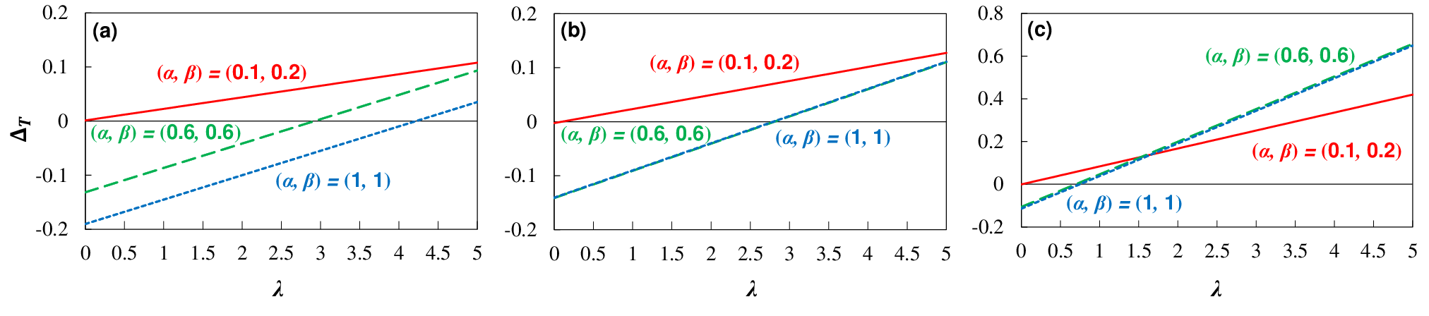
Figure 9 plots for (a) , (b) , and (c) as functions of for various , which are plotted as black crosses in Fig. 8. We emphasize again that in the region with group sequences are preferred, even if when the sorting cost is considered, whereas in the region with random sequences are preferred. Note that the cases with correspond to those obtained without considering the sorting cost.
As discussed in the previous subsection, we note that for almost all when , indicating that sorting is almost always beneficial for smooth transportation. However, once the sorting cost is considered, the sign of can become positive, especially in the region where is relatively small, indicating that sorting is not always beneficial. Note that the curves of (0.6, 0.6) and (1, 1) are observed to overlap each other in Fig. 9 (b) and (c), unlike Fig. 9 (a). This happens because there is no difference in at these two points when , as we can see in Figs. 8 (b) and (c).
Figure 10 plots for (a) , (b) , and (c) for various with . In this figure, we note the existence of a new region in which , which we term a ‘random-advantageous region’ (). This new region widens as increases, finally resulting in the complete disappearance of the group-advantageous region for large enough . Note that Fig. 10 (c) exhibits only a random-advantageous region.
IV THEORETICAL ANALYSES
In this section, we show that the simulation results can be theoretically reproduced in some special cases. Specifically, we have succeeded in obtaining a mathematical proof of the appearance of the group-advantageous region for any group number when .
IV.1 Approximate flow of a multi-species TASEP
In this subsection, before calculating , we briefly discuss the steady-state flow of the multi-species TASEP that corresponds to a random sequence. We write , with the arguments abbreviated in obvious cases. When the flow is simulated for each parameter set, we first evolve the system for time steps and then average over the next time steps.

IV.1.1
This subsection presents the derivation of an approximate based on a Markov chain model. Due to the difficulty of considering general values of (the length of the lattice) and (the number of particle species), we consider the simplest case—with and . As two species of particles exist—that is, particles with hopping probability and particles with —each site may have three states: ‘unoccupied (state 0),’ ‘occupied by a particle 1 (state 1),’ and ’occupied by a particle 2 (state 2).’ This results in 9 possible states; however, noting that it is not necessary to distinguish the particle at site 1 because it always leaves the lattice with probability , the number of possible states can be reduced to 6. Here, we define the probability distribution (), where and represent the state number of site 0 and 1, respectively. Note that state indicates either of state 1 or 2.
The master equations for the steady state are summarized in Eq. (2), using the relation . Note that and are replaced with and , respectively, for the case . In addition, must satisfy the normalization condition
| (3) |
From Eqs. (2) and (3), the flow of the system can be written as a function of , , and ; that is, , is given by the following expression:
| (4) |
where
For and , the system reduces to the single-species TASEP with the flow , where
| (7) |
Note that the flow of the single-species TASEP for general is exactly solved in Ref. Evans et al. 1999. Therefore, assuming that the value satisfies the condition , we can derive
| (8) |
The quantity is termed the harmonic mean of and . Accordingly, for , is equivalent to . This relation holds for any species number , as we show in Appendix D.
Figure 11 compares the simulation and theoretical curves for various with (a) , (b) and (c) . In all the figures, the simulations show very good agreement with our exact analyses.


IV.1.2 General
For general and , it is complicated to solve the master equations. Therefore, in this subsection, we instead assume an inequality, based on the results in the previous subsection and the qualitative discussions, and confirm the validity of the inequality by the simulations.
First, for general and , is clearly larger than , where .
In addition, for , a platoon can be observed in the bulk of the lattice, in which a slower particle behaves as a bottleneck, and faster particles behind it cannot hop with a probability larger than that of the smaller one, i.e., less than , as shown in Fig. 12. This phenomenon suppresses the flow, implying that is smaller than .
Consequently, satisfies the following inequality;
| (9) |
In this subsection, we hereafter consider the case .
Figure 13 shows the phase diagrams obtained by plotting the simulation values for (a) the single-species TASEP with , (b) the two-species TASEP, and (c) the single-species TASEP with , respectively. Note that () are the simulation (theoretical) values (and similarly hereafter).
Comparing these three figures shows that Eq. (9) obviously holds. In addition, as in Figs. 13 (a) and (c), we find that three different phases—HD, LD, and MC—also exist in Fig. 13 (b). Due to Eq. (9), the boundaries between the LD (HD) and MC phases of Fig. 13 (b) lie between those of Figs. 13 (a) and 13 (c). Note that the black lines in Figs. 13 (a) and (c) are theoretical boundaries, based on the fact that the boundary between the LD and MC phases of the single-species TASEP with hopping probability de Gier and Nienhuis 1999 can be written as
Here, as for , we define as the ratio of the change from to ; that is,
| (13) |
and we note that when .
Figure 14 shows for various (), for the fixed parameter set . The black lines represent the boundaries between the LD/HD and MC phases of the single-species TASEP with hopping probability (boundary 1) and the single-species TASEP with (boundary 2). Therefore, the lower-left (upper-right) region beyond boundary 1 (boundary 2) corresponds to the LD/HD (MC) phases both for the two-species TASEP and for the single-species TASEP with . This figure confirms that starts from 0 in the LD/HD phase, decreases, and finally yields to a constant value in the MC phase as approaches the upper right.
Figure 15 plots as a function () for various , fixing . Note that both the single-species TASEP with hopping probability and the two-species TASEP exhibit the LD, HD, and MC phases with (0.1, 0.2), (0.2, 0.1), and (1, 1), respectively. This is because . For example, Fig. 13 confirms that those three points exist within each corresponding phase for .
In Figs. 15 (a) and (b), we find that is approximately 0, whereas deviates from 0 in Fig. 15 (c), as is also observed in Fig. 14. These phenomena can be explained as follows.
First, in the LD/HD phase, is mainly governed by the input/output probability, leading to , i.e., approaches . This is because deviates from mainly due to the existence of platoons, which do not influence the flow much in this phase. Note that decreases as or approaches 0.2, because the influence of platoons increases, approaching the MC phase of the two-species TASEP.
On the other hand, in the MC phase, is mainly governed by the bulk region of the lattice. Therefore, the existence of platoons has a more critical influence on , causing to deviate from 0; i.e., . Especially as increases, the extent of the deviation also increases. This is because the effect of platoons increases when there is a large gap between and .
Figure 16 plots (a) , (b) , and (c) for various . Both of () and are obtained by the simulations. In all the figures, we observe that for , generally becomes less than 1, i.e., , especially when increases, i.e., the system approaches and exhibits the MC phase. Note that for , the difference among is unclear; however, it becomes obvious when . Those results imply that Eq. (9) and its qualitative discussions can be applicable for general and .
IV.2 Relation between and
without the sorting cost
Hereafter, we assume , , , and .
In this subsection, we fix , i.e., we do not consider the sorting cost. If for any number of particle species , is large enough for and to be determined by the steady-state flow (see Appendix E), we obtain
| (14) |
and
| (15) |
Note that this approximation immediately implies the independence of from the order of the group sequence. Strictly speaking, can differ depending on the order of each group in the group sequence. However, that difference can be ignored for large (see Appendix E).
In addition, we define the transportation times of the particles with the same hopping probabilities and as
| (16) |
and
| (17) |
respectively. From Eqs. (9), (14), (16) and (17), we immediately obtain the inequality
| (18) |
In the following, we show that a general relation between and can be obtained mathematically for general . We emphasize that this relation can be proven by comparing and , and not by comparing and directly. Here, we introduce the new function , which is defined as follows:
| (19) |
Because we can assume without loss of generality, we adopt this assumption in the following discussion, writing in abbreviated form . Note that for cases with , the theoretical results can be obtained simply by replacing (LD) with (HD).
A contour map of in the plane exhibits four large regions, which are summarized in Tab. 1.
| Region No. | Range |
|---|---|
| 1 | |
| 2 | |
| 3 | |
| 4 |
In the following subsections, we examine the behavior of according to this classification.
IV.2.1 Region 1:
In this region, all the steady-state phases of the single-species TASEP for any exhibit the LD phase. Here, the steady-state flow for the single-species TASEP with parallel updating de Gier and Nienhuis 1999 is given by
Therefore, we obtain
IV.2.2 Region 2:
This region is further divided into () subregions, as summarized in Tab. 2.
| Subregion No. | Range |
|---|---|
| 2– | |
| 2– | |
| … | … |
| 2– | |
| … | … |
| 2– |
In Subregion 2– (), the single-species TASEP with exhibits the MC phase, whereas that with displays the LD phase. Therefore, using Eq. (IV.2.1), we obtain
From Eqs. (15), (16), and (IV.2.2), and can be written as follows;
| (30) |
and
| (31) |
From Eqs. (30) and (31), we thus obtain in the form
| (32) |
For , due to and , we obtain for and . The function is continuous and differentiable with respect to , including at each boundary (see Appendix G). However, the signs of and are not specified. Note that the following condition
| (33) |
where indicates that increases monotonically at least near the boundary between Subregion 2–() and Region 3. This is discussed in Appendix H.
IV.2.3 Region 3:
Similarly to Region 2, this region is further divided into () subregions, as summarized in Tab. 3. Note that Subregion 3–1 vanishes in the case , resulting in () subregions.
| Subregion No. | Range |
|---|---|
| 3– | |
| 3– | |
| … | … |
| 3– | |
| … | … |
| 3– |
In Region 3– (), the single-species TASEP with exhibits the MC phase, whereas that with displays the LD phase. Therefore, using Eq. (IV.2.1), we obtain
From Eqs. (15), (16), and (IV.2.3), and can be written as follows;
IV.2.4 Region 4:
In this region, all the steady-state phases of the single-species TASEP for any hopping probabilities and exhibit the MC region. Note that this region vanishes in the case because .
Therefore, we obtain
| (43) |
IV.2.5 Relation between and
With the results of Subsec. IV.2.1–IV.2.4, we can obtain a general relation between and for some special cases. Table 4 summarizes the signs of and in each region. Note that ‘U’ indicates that the sign is unclear.
| Region No. | ||
| 1 | U | |
| 2 | U | U |
| 3 | U | |
| 4 | 0 |
Considering Tab. 4 and the continuity of including at each boundary (see Appendix G), we find from the intermediate value theorem that such that satisfies
| (45) |
in Region 2 or 3. The specific conditions that must satisfy are given in Appendix K.
Defining as the largest value among the quantities , we obtain —i.e., —in the region where . This is because is continuous and increases monotonically from a point in Region 2 (and through Region 3), to yield in Region 4.
Considering Eq. (18), we finally obtain
| (46) |
in the region . Eq. (46) means that , reproducing the simulation results in the region where is relatively large. This result indicates that the group-advantageous region must appear even in a case with , for which Region 4 vanishes.
In analogy with the discussion above, we can also predict that a region with must appear in the case .
IV.3 Relation between and with sorting cost
In this subsection, we discuss the change in the relation between and when , i.e., when the sorting cost is included. In the following, we first obtain a general formula for the sorting cost and then evaluate upper and lower limits to .
IV.3.1 General formula for the sorting cost
First, we calculate mathematically the averaged minimal number of exchanges necessary to sorting the particles from random to group sequences.
We here define as the averaged value of , using the fact that can take patterns with equal probability. We thus have
| (47) |
If is the minimal number of exchanges necessary to sort the particles from a random sequence to a given fixed group sequence , then satisfies
| (48) |
Note that the number of elements of is equal to that of from the definition. Eqs. (47) and (48) indicate that the best group sequence can vary depending on the particular random sequence .
Due to the difficulty of a general calculation of , we instead calculate , which is defined as follows:
| (49) |
where is a fixed sequence out of the set {} for all possible .
For and , can be generally calculated as
the detailed derivations of which are discussed in Appendix L.
Figure 17 shows the ratio for (a) and (b) . Both figures show that , i.e., , indicating that there is no problem in substituting for for large enough .
In the following calculations, we therefore use instead of because can be represented by a general formula, whereas cannot.


IV.3.2 Upper and lower limits to
We first define , as the value for which . Note that is defined to be equal to 0 if when . From the definition of , the random-advantageous region appears when . Based on the discussions in Subsec. IV.2 and IV.3.1, we here evaluate for and .
To take into account the sorting cost, we add the term to ; that is,
| (53) |
Conversely, we do not add that term to because a random sequence means a sequence without sorting.
We also define and as the values of for which and , respectively. Note that can have negative values, because can be less than .
| Region No. | Upper and lower limits to |
|---|---|
| 1 | |
| 2 | |
| 3 | |
| 4 |

From Eq. (18) and Subsec. IV.2, when the relations among , , , and must satisfy one of the following three inequalities:
| (54) |
| (55) |
or
| (56) |
Therefore, the relations of , , and can be written as follows:
| (57) |
where we note that by definition , whereas can be either negative or positive, while must be positive.
In Region 1, i.e., , where with , must be negative, while must be positive, and satisfy
| (58) |
In Region 2, i.e., , can be either negative or positive, whereas must be positive. The quantities and satisfy
| (59) |
and
| (60) |
respectively.
In Region 3, i.e., , can be either negative or positive, and must be positive. Thus, and satisfy
| (61) |
and
| (62) |
respectively.
In Region 4, i.e., , due to when , and must both be positive. The quantities and therefore satisfy
| (63) |
and
| (64) |
respectively.
Table VI summarizes the upper and lower limits to in each region. Furthermore, Fig. 17 shows the simulation values (black circles) and the theoretical existence range of (yellow region) as functions of . Note that the we calculated the simulation values using with 10-trial-averaged values of , , and .
We can interpret Fig. 17 as demonstrating that a group (random) sequence is preferable in the region below (above) the black line. In the blue (green) region, a group (random) sequence is in fact theoretically verified to be preferable. Comparing Figs. 17 (a) and (b), the simulation values approach the lower limit—i.e., the accuracy of approximating by increases—as decreases. We admit that the yellow region is extensive, especially when is relatively large; however, we emphasize that the simulation values always exist within the expected region and that the region can be limited easily without numeric calculations, which is convenient for applications to actual situations.
V CONCLUSION
In the present study, we have used a modified TASEP to analyze the dependence of the transportation time on the entering sequences of particles, using both the numerical simulations and theoretical analyses.
Here, we summarize a number of important results. In Sec. III, we discovered that there exists an important ‘group-advantageous region’ where when is relatively large and the sorting costs are neglected. When sorting costs are introduced, a new region called a ‘random-advantageous region’ appears with . In addition, the group-advantageous region shrinks and finally disappears as increases. We explored these phenomena for various .
In Sec. IV, we analyzed the simulation results by employing mathematical approaches for certain special cases. Using some approximations, we have shown theoretically that without the sorting cost the group-advantageous region must appear for any parameter sets (). Moreover, we have succeeded in deriving the upper and lower limits to the value of where by obtaining a general formula for the sorting cost.
Our findings can be applied to real-world situations, such as providing efficient operation for various tasks and smooth logistics for various products and yielding an effective evacuation method for pedestrians. Specifically, for smooth operation, we can determine whether we should begin tasks without considering the operation sequence or otherwise. Similarly, for smooth logistics, we can select whether the products should be bunched with nearly equal sizes. Furthermore, for ensuring effective evacuation of pedestrians, we can determine whether the bunching of pedestrians having nearly equal velocities should be conducted before transportation. The criteria for these judgments depend on the magnitude of the consideration or bunching cost (). Note that these magnitudes significantly differ from each other, i.e., considering only the sequence of tasks is typically deemed cheaper (have a smaller ) than sorting various pedestrians and products.
ACKNOWLEDGMENTS
This work was partially supported by JST-Mirai Program Grant Number JPMJMI17D4, Japan, JSPS KAKENHI Grant Number JP15K17583, and MEXT as ’Post-K Computer Exploratory Challenges’ (Exploratory Challenge 2: Construction of Models for Interaction Among Multiple Socioeconomic Phenomena, Model Development and its Applications for Enabling Robust and Optimized Social Transportation Systems) (Project ID: hp180188).
Appendix A Validity of our selection of and
In this Appendix, we briefly discuss the validity of selecting and .
As finite-size effects may occur for small , we compare the simulation values of for and . Figure 18 shows the ratio , where and represent the flow of the multi-species TASEP with and , respectively, as functions of for various . The result that indicates that the effect can be ignored for . Thus, we choose to decrease the simulation time.

On the other hand, the assumption that is determined by a steady-state flow may be inappropriate for small . Therefore, we have compared the results for and , in both cases for . Figure 19 shows the ratio , where and represent the transportation times for and , respectively, as functions of for various . The result that , i.e., that is proportional to , indicates that the assumption can be regarded as valid for . Thus, we choose similarly to decrease the simulation time.

Appendix B Simulation schemes for obtaining the minimal number of necessary exchanges
In this Appendix, we briefly describe the specific simulation schemes we used to obtain . We emphasize that the cost of counting or comparing particles and the distances between exchanged particles are both ignored in the following.
First, for , can have only one of two patterns. Once is fixed to be either of these two sequences, we can immediately obtain the number of particles placed at the wrong areas in sequence , which is twice as large as the number of necessary exchanges (see also Appendix L). Consequently, comparing the results for the two gives the smaller number as .
Second, for , can have six patterns. Once is fixed at one of these six sequences, we can immediately obtain the number of particles placed at the wrong areas in any sequence . After selecting one species, which we first replace at the correct location, we exchange all particles of that species that are placed in the wrong areas in sequence . The subsequent procedure is similar to the case for . Consequently, comparing the six results for each again gives the smallest number as . Note that we can similarly calculate the numbers for general .
Finally, for , can have one of two patterns: either an ascending or a descending sequence. One exchange is needed for each particle in for which there exists a particle with a smaller (larger) hopping probability than the noted particle. This is termed a ‘selection sort.’ This procedure starts from the leading particle. Consequently, by comparing the results for the two , the smaller number is again selected as the minimal number of necessary exchanges.
Appendix C Probability distribution with and
Here, we summarize the probability distributions with and , which can be obtained from Eqs. (2) and (3). The specific forms are described as follows:
| (65) |
where
| (66) |
| (67) |
and
| (68) |
Appendix D for general with
In this appendix, we prove that for general with , is equal to .
From the results with and (see Appendix C), we can conjecture the probability distributions for general with as
| (69) |
where .
On the other hand, the master equations of the steady state are summarized as equations:
| (70) |
where . In addition, must satisfy the normalization condition
| (71) |
We can confirm that Eqs. (69) satisfy Eqs. (70) and (71). With Penron-Frobenius theorem regarding stochastic matrix, this indicates that Eqs. (69) are unique solutions for Eqs. (70) and (71).
From Eqs. (69), the flow of the system is given by the following expression:
| (72) |
Appendix E Validity of the approximation for
In this Appendix, we briefly demonstrate the validity of Eq. (15).
Figure 20 (a) shows the ratio as a function of for various with and Fig. 20 (b) shows the same ratio for . Note that and represent the values of from the simulations and that given by Eq. (15), respectively. Both figures show that , indicating that Eq. (15) provides a good approximation for .


Strictly speaking, must be larger than 1 on average. This is mainly due to the fact that includes , which is the time required for the first particle to reach the right-hand boundary, whereas ignores that time. This also indicates that can differ depending on the order of each group in the group sequence (i.e., the hopping probability of the leading group). However, this difference has little influences on the theoretical results, as explained below.
First, can be estimated as
| (73) |
where and the time steps before the first particle enters the lattice are assumed to be small enough to be ignored. The quantities and without satisfy
| (74) |
and
| (75) |
respectively. Therefore, reduces to
| (76) |
Under the proposition that is large enough, we can assume ( in the present study). In fact, observing the time series of the flows (199-steps central moving average) in Fig. 21, we find that nearly the entire duration during transportation can be regarded to be in the steady state for large enough . Note that we calculate the flows at time by averaging number of moving particles per bond between and . Moreover, all the transportation times (, , and ) originally include , so that this term disappears when they are subtracted from each other. Consequently, (and therefore, the dependence of on the order of each group in the group sequence) can be assumed to be ignorable.

Appendix F Discussion of the sign of
in Region 1
In this Appendix, we give a detailed derivation of Eq. (26) for Region 1, where .
Eq. (25) gives
| (77) |
where
| (78) |
The quantity is calculated as follows:
| (79) |
where
| (80) |
By regarding the sum of the term with and that with as a new term for , we can rewrite Eq. (79) as follows:
| (81) |
Because () and , we obtain .
Considering and , we finally obtain
| (82) |
Appendix G Continuity and differentiability of at each boundary
In this Appendix, we briefly discuss the continuity and differentiability of at each boundary.
Defining for as
where , the following equations hold:
| (86) |
and
| (87) |
where . Therefore, is continuous and differentiable at , resulting in the continuity and differentiability of for .
As a result, because is represented as a linear sum of terms , where is substituted for or (), is clearly continuous and differentiable at each boundary.
Appendix H Discussion of the sign of
in Subregion 2–
In this Appendix, we discuss the sign of in Subregion 2–, i.e.,
From Eq. (32), can be calculated as follows:
| (88) |
For , the following two inequalities hold:
| (89) |
and
| (90) |
Appendix I Discussion of the sign of
in Subregion 3–
In this Appendix, we give a proof on Eq. (40) in Subregion 3–, i.e., .
From Eq. (39), can be calculated as follows:
Appendix J Discussion of the sign of
in Region 4
In this Appendix, we give a detailed derivation of Eq. (44), where .
| (98) |
where
| (99) |
and
| (100) |
From Eqs. (99) and (100), becomes
| (101) |
Here, regarding the sum of the term with and that with as a new term for , Eq. (101) can be rewritten as
| (102) |
Due to Eq. (102) and the non-negativity of both and , we have , thereby resulting in
| (103) |
Appendix K Specific conditions on
Here, we discuss the specific conditions on .
Table VI summarizes explicit expressions for , where the upper (lower) expression holds in Region 2 (Region 3). For , the lower expression becomes a quadratic equation in . However, the upper expression becomes a quartic equation that is too difficult to solve analytically those conditions. Note that for , both equations become more than quartic.
From its definition of , can be written as
| (104) |
where represents the set of .
| Region No. | Explicit expressions for | ||
|---|---|---|---|
| 2 |
| ||
| 3 |
|
Appendix L Derivation of
In this Appendix, we derive the approximate averaged minimal number of exchanges necessary to sort the particles for two special cases: and .
L.1
First, for a general calculation of , has to be fixed to be either of the two possible patterns. Once is fixed, can be determined uniquely for all possible . Without loss of generality, we can assume and can be fixed as illustrated in the lower panel of Fig. 22.

Suppose that for , particles of species 1 are located in the Area 2, ( particles of species 2 are located in the Area 1, conversely) as described in the lower of Fig. 22. Under this supposition, -time exchanges are necessary for sorting particles from to . Considering that satisfying this supposition possibly has sequences, can be written as follows;
| (105) |
Using the Vandermonde convolution formula, Eq. (105) can be rewritten as follows:
| (106) |
Because the sequence can take any of possible patterns with equal probability, we can finally reduce to
| (107) |
Figure 23 compares the simulation (circles) and theoretical (curves) values for various for . The simulations show very good agreement with our exact analysis.

L.2
When , also has to be fixed as either of the two possible patterns—an ascending or a descending sequence—for a general calculation of , as illustrated in the upper panel of Fig. 24. Once is fixed, can be determined uniquely for all possible .

If we regard the entire sequence as consisting of two parts—the first (blue) particle and other () particles, as described in the lower panel of Fig. 24—the sorting procedure can also be divided into two parts: sorting () particles plus the last exchange for the first particle. If the first particle corresponds to the particle with hopping probability , and noting that the sequence for the remaining () particles has possible patterns, we can calculate the quantity as follows:
| (108) |
where and represents the sequence for which the first particle is the particle with hopping probability . Note that the last sort is not necessary in the case where .
Therefore, for , we can write :
| (109) |
Dividing both sides of Eq. (109) by , we obtain
| (110) |
where and . With the initial condition , is finally reduced to
| (111) |
which we note holds for the case .
The sequence can take patterns with equal probability, and therefore, is finally reduced to
| (112) |
Figure 25 compares the simulation (circles) and theoretical (line) values for . The simulations again show a very good agreement with our exact analysis.

References
- Appert-Rolland et al. (2017) C. Appert-Rolland, S. Klein, M. Ebbinghaus, and L. Santen, in Proceedings of the Asia-Pacific Econophysics Conference 2016 Big Data Analysis and Modeling toward Super Smart Society (APEC-SSS2016) (2017) p. 011001.
- Croom et al. (2000) S. Croom, P. Romano, and M. Giannakis, Eur. J. Purch. Supply Manag. 6, 67 (2000).
- Ezaki et al. (2015) T. Ezaki, D. Yanagisawa, and K. Nishinari, Physica A 427, 62 (2015).
- Taniguchi et al. (2015) Y. Taniguchi, R. Nishi, T. Ezaki, and K. Nishinari, Physica A 433, 304 (2015).
- Woelki (2013) M. Woelki, Phys. Rev. E 87, 062818 (2013).
- Imai and Nishinari (2015) T. Imai and K. Nishinari, Phys. Rev. E 91, 062818 (2015).
- Yamamoto et al. (2017) H. Yamamoto, D. Yanagisawa, and K. Nishinari, J. Stat. Mech. 2017, 043204 (2017).
- Christensen and Sasaki (2008) K. Christensen and Y. Sasaki, J. Artif. Soc. Soc. Simul. 11, 9 (2008).
- Pelechano and Malkawi (2008) N. Pelechano and A. Malkawi, Automat. Constr. 17, 377 (2008).
- Yanagisawa et al. (2009) D. Yanagisawa, A. Kimura, A. Tomoeda, R. Nishi, Y. Suma, K. Ohtsuka, and K. Nishinari, Phys. Rev. E 80, 036110 (2009).
- Ezaki et al. (2012) T. Ezaki, D. Yanagisawa, K. Ohtsuka, and K. Nishinari, Physica A 391, 291 (2012).
- Rothman (1994) J. E. Rothman, Nature 372, 55 (1994).
- Müller et al. (2008) M. J. Müller, S. Klumpp, and R. Lipowsky, Proc. Natl. Acad. Sci. 105, 4609 (2008).
- Bressloff and Newby (2013) P. C. Bressloff and J. M. Newby, Rev. Mod. Phys. 85, 135 (2013).
- MacDonald et al. (1968) C. T. MacDonald, J. H. Gibbs, and A. C. Pipkin, Biopolymers 6, 1 (1968).
- MacDonald and Gibbs (1969) C. T. MacDonald and J. H. Gibbs, Biopolymers 7, 707 (1969).
- Parmeggiani et al. (2003) A. Parmeggiani, T. Franosch, and E. Frey, Phys. Rev. Lett. 90, 086601 (2003).
- Chowdhury et al. (2005) D. Chowdhury, A. Schadschneider, and K. Nishinari, Phys. Life Rev. 2, 318 (2005).
- Chou et al. (2011) T. Chou, K. Mallick, and R. Zia, Rep. Prog. Phys. 74, 116601 (2011).
- Appert-Rolland et al. (2015) C. Appert-Rolland, M. Ebbinghaus, and L. Santen, Phys. Rep. 593, 1 (2015).
- Helbing (2001) D. Helbing, Rev. Mod. Phys. 73, 1067 (2001).
- Ito and Nishinari (2014) H. Ito and K. Nishinari, Phys. Rev. E 89, 042813 (2014).
- Tsuzuki et al. (2018) S. Tsuzuki, D. Yanagisawa, and K. Nishinari, Phys. Rev. E 97, 042117 (2018).
- Yanagisawa et al. (2010) D. Yanagisawa, A. Tomoeda, R. Jiang, and K. Nishinari, JSIAM Lett. 2, 61 (2010).
- Arita and Yanagisawa (2010) C. Arita and D. Yanagisawa, J. Stat. Phys. 141, 829 (2010).
- Arita and Schadschneider (2015) C. Arita and A. Schadschneider, Math. Mod Meth. 25, 401 (2015).
- de Gier and Nienhuis (1999) J. de Gier and B. Nienhuis, Phys. Rev. E 59, 4899 (1999).
- Blythe and Evans (2007) R. A. Blythe and M. R. Evans, J. Phys. A 40, R333 (2007).
- Derrida et al. (1993) B. Derrida, M. R. Evans, V. Hakim, and V. Pasquier, J. Phys. A 26, 1493 (1993).
- Minemura et al. (2010) T. Minemura, K. Nishinari, and A. Schadschneider, in International Conference on Cellular Automata (Springer, 2010) pp. 593–599.
- Adams et al. (2008) D. A. Adams, B. Schmittmann, and R. K. P. Zia, J. Stat. Mech. 2008, P06009 (2008).
- Cook et al. (2009) L. J. Cook, R. K. P. Zia, and B. Schmittmann, Phys. Rev. E 80, 031142 (2009).
- Cook and Zia (2009) L. J. Cook and R. K. P. Zia, J. Stat. Mech. 2009, P02012 (2009).
- Cook and Zia (2012) L. J. Cook and R. K. P. Zia, J. Stat. Mech. 2012, P05008 (2012).
- Angel (2006) O. Angel, J. Comb. Theory A 113, 625 (2006).
- Ferrari et al. (1994) P. A. Ferrari, L. R. Fontes, and Y. Kohayakawa, J. Stat. Phys. 76, 1153 (1994).
- Arita (2006) C. Arita, J. Stat. Mech. 2006, P12008 (2006).
- Mallick (1996) K. Mallick, J. Phys. A 29, 5375 (1996).
- Derrida and Evans (1999) B. Derrida and M. Evans, J. Phys. A 32, 4833 (1999).
- Ayyer et al. (2009) A. Ayyer, J. L. Lebowitz, and E. R. Speer, J. Stat. Phys. 135, 1009 (2009).
- Privman (2005) V. Privman, Nonequilibrium statistical mechanics in one dimension (Cambridge University Press, 2005).
- Ferrari et al. (2007) P. A. Ferrari, J. B. Martin, et al., Ann. Probab. 35, 807 (2007).
- Cantini (2008) L. Cantini, J. Phys. A 41, 095001 (2008).
- Uchiyama (2008) M. Uchiyama, Chaos Soliton Fract. 35, 398 (2008).
- Crampe et al. (2015) N. Crampe, K. Mallick, E. Ragoucy, and M. Vanicat, J. Phys. A 48, 175002 (2015).
- Aneva (2003) B. Aneva, Eur. Phys. J. C 31, 403 (2003).
- Arita et al. (2009) C. Arita, A. Kuniba, K. Sakai, and T. Sawabe, J. Phys. A 42, 345002 (2009).
- Duchi and Schaeffer (2005) E. Duchi and G. Schaeffer, J. Comb. Theory A 110, 1 (2005).
- Evans (1997) M. Evans, J. Phys. A 30, 5669 (1997).
- Krug and Ferrari (1996) J. Krug and P. A. Ferrari, J. Phys. A 29, L465 (1996).
- Mallick et al. (1999) K. Mallick, S. Mallick, and N. Rajewsky, J. Phys. A 32, 8399 (1999).
- Crampe et al. (2016) N. Crampe, C. Finn, E. Ragoucy, and M. Vanicat, J. Phys. A 49, 375201 (2016).
- Arita and Mallick (2013) C. Arita and K. Mallick, J. Phys. A 46, 085002 (2013).
- Prolhac et al. (2009) S. Prolhac, M. R. Evans, and K. Mallick, J. Phys. A 42, 165004 (2009).
- Ayyer and Roy (2017) A. Ayyer and D. Roy, Sci. Rep. 7, 13555 (2017).
- Arndt et al. (1998) P. F. Arndt, T. Heinzel, and V. Rittenberg, J. Phys. A 31, L45 (1998).
- Evans (1996) M. Evans, Europhys. Lett. 36, 13 (1996).
- Sasamoto (2000) T. Sasamoto, Phys. Rev. E 61, 4980 (2000).
- Bengrine et al. (1999) M. Bengrine, A. Benyoussef, H. Ez-Zahraouy, J. Krug, M. Loulidi, and F. Mhirech, J. Phys. A 32, 2527 (1999).
- Duchi and Schaeffer (2008) E. Duchi and G. Schaeffer, Random Struct. Algor. 33, 434 (2008).
- (61) To be precise, if we regard vacant sites as particle 0, swapping between particle 0 and other kinds of particles (1, 2, 3,……) occurs. However, swapping between particles 1, 2, 3,…… does not occur.
- (62) This system can be simulated also with random updating; however, we adopt parallel updating for the following three reasons. First, we consider that the results will be mainly applied to real systems, where particles and agents move simultaneously. It is generally natural to adopt parallel updating in the contexts of pedestrian dynamics or traffic flows Nagel and Schreckenberg 1992; Burstedde et al. 2001. Second, it is more natural to consider that time for swapping two particles is compatible with a one-time step with parallel updating than with random-sequential updating. Finally, the simulation times can be suppressed drastically with parallel updating compared to with random updating.
- Evans et al. (1999) M. R. Evans, N. Rajewsky, and E. R. Speer, J. Stat. Phys. 95, 45 (1999).
- Nagel and Schreckenberg (1992) K. Nagel and M. Schreckenberg, J. de Phys. I 2, 2221 (1992).
- Burstedde et al. (2001) C. Burstedde, K. Klauck, A. Schadschneider, and J. Zittartz, Physica A 295, 507 (2001).