Optimisation of hierarchical dielectric elastomer laminated compositesPublished in International Journal of Non-Linear Mechanics, Volume 106, November 2018, Pages 266-273, doi: 10.1016/j.ijnonlinmec.2018.06.005

The application of electro-elasticity theory of soft dielectrics [1, 2] to the area of heterogenous materials has already shown that suitably designed microstructured composites may potentially exhibit remarkably improved actuation properties with respect to those displayed by the homogeneous materials employed so far, mainly acrylic elastomers and silicones [3]–[14]. Some of these studies also investigated the shortcomings associated with the use of composites that are related to peculiar phenomena such as the triggering of micro-, macro-scopic and electro-mechanical instabilities, electric field amplification inside some constituents, etc. [4, 5, 8, 9, 10, 12].

A significant part of the research on heterogeneous soft dielectrics has been devoted to (hierarchical) layered composites. Working in the small-strain setting, Tian et al. [7] have shown that two-phase dielectric rank-$n$ laminate layouts (with $n>1$) can be found to improve the electro-mechanical actuation strain of more than one order of magnitude at the same voltage (being the gain strongly related to the order $n$ of the microstructure). Or, in other words, that, in a rank-two laminate, the actuation enhancement obtained at an increasing contrast in the electro-mechanical properties of phases is more than proportional, almost linear in a graph where actuation strain and contrast are reported with a logarithmic scale.

In the more appropriate finite-strain, non-linear framework, laminated composites have been studied by some authors extending the methodology set out by deBotton [15]: deBotton et al. [3] provided the first preliminary analysis of the behaviour of rank-one laminates; Bertoldi and Gei [4], Rudykh and deBotton [5], Gei et al. [9], Rudykh et al. [10] and Spinelli and Lopez-Pamies [12] investigated in detail the homogenisation and the micro- and macro-scopic stability of layered composites. An evaluation of the benefit of the hierarchical structure of a rank-two composite in the electro-mechanical actuation has been carried out by Rudykh et al. [8] who have found a ten-fold improvement of the electro-mechanical coupling for a prototype laminate obtained by reinforcing with polyaniline an acrylic elastomer matrix.

This paper deals with the optimisation of the actuation response of rank-two dielectric laminates in the non-linear framework of finite electro-elasticity under both plane strain and three-dimensional unconstrained boundary conditions. The main goals are:

– to extend the analysis of the optimisation of rank-two laminates presented in [7] to better assess the gain in large-strain actuation with respect to both the homogeneous and the rank-one response;

– to establish the optimum configurations of the composite for different contrasts between the soft matrix and the stiff reinforcement;

– to show that those configurations strongly depend on the maximum operational electric field chosen for the actuator;

– to evaluate the amplification of the current electric field in some representative configurations to provide an indication of the effective local electro-mechanical response.

We are not concerned here with occurrence of any instability or other failure mode along the electro-mechanical actuation path, but we recognise that any departure from the homogeneous response may have a strong impact in the evaluation of the optimum layout.

Two material combinations are considered in the examples: one is that adopted by Tian et al. [7], characterised by a matrix whose electro-mechanical properties match those of a polyurethane, for which the authors analysed several configurations with equal contrast between shear moduli and electric permittivities; the other possesses a softer, silicone-like matrix, reinforced with a stiffer phase which may correspond to a poly(vinylidene fluoride) electrostrictive polymer [16].

The general layout of the hierarchical composite actuator under investigation is represented in Fig. 1, where $h^{0}$ is the reference thickness. The laminate is constructed layering two phases: $a$, the reinforcement, and $b$, the matrix, usually softer than phase $a$ and with a lower electric permittivity, in a manner consistent to the scheme called ‘tree a’ in [7]. According to this scheme, the final layout is obtained layering a parent rank-one composite (the core, abbreviated to ‘co’, whose volume fraction will be denoted by $c^{\rm co}$) with a layer of soft material acting as a shell (abbreviated to ‘sh’, with volume fraction $c^{\rm sh}$ such that $c^{\rm sh}+c^{\rm co}=1$). In [7], this layout has proven to give better performance than that of another type of arrangement, called ‘tree b’. It is clear that while the materials to be mixed are two, namely, $a$ and $b$, the device is composed of three parts, i.e. $a$, $b^{\rm co}$ and $b^{\rm sh}$, with $b^{\rm sh}$ coinciding with the shell. To complete the description of the notation related of volume fractions, $c_{a}^{\rm co}$ and $c_{b}^{\rm co}$ denote, in turn, the volume fractions of $a$ and $b$ in the core, whilst $c^{a}=c_{a}^{\rm co}$ and $c^{b}=c_{b}^{\rm co}+c^{\rm sh}$ are the total volume fractions of the two phases ($c^{a}+c^{b}=1$). The grades with respect to the axis $x_{1}$ of the interfaces between $a$ and $b$ in the core and of the shell correspond to $\theta_{\rm co}$ and $\theta_{\rm sh}$, respectively. Separation of length-scales is assumed so that homogenisation at each rank can be invoked. The theory here recalled for the solution of the electro-elastic problem for hierarchical composites relies on the formulation that can be found in [6, 11, 12, 15], for which the effective properties can be obtained exactly up to a set of algebraic equations.

A notation which is standard in large-strain electro-elasticity is adopted¹¹ 1 see [9]. Boldface letters $\mbox{\boldmath${\it x}$}^{0}$ and ${\it x}$ represent points of $B^{0}$ and of the current configuration $B$, respectively, while differential operators with capital letters are evaluated with reference to $B^{0}$.. Symbols $\mbox{\boldmath${\it D}$}^{0}$ and $\mbox{\boldmath${\it E}$}^{0}$ denote, in general, nominal electric displacement and nominal electric fields, respectively, while ${\it S}$ and ${\it F}$ stand for the total first Piola-Kirchhoff stress tensor and the deformation gradient, respectively. As they were introduced, without any subscript, those four quantities are referred to the macroscopic response of the composite whereas, when accompanied by a subscript, they are referred to the indicated constituent so, e.g. $\mbox{\boldmath${\it F}$}_{k}={\rm Grad}\,\mbox{\boldmath${\it x}$}_{k}\ (k=a,b^{\rm co},b^{\rm sh})$ denotes the local deformation gradient that, together with the local nominal electric field $\mbox{\boldmath${\it E}$}^{0}_{k}$, is assumed to be constant in each part. Both phases $a$ and $b$ obey an extended neo-Hookean strain-energy function formulated for incompressible materials, namely

$$W_{k}=\frac{\mu_{k}}{2}(\mbox{\boldmath${\it F}$}_{k}\mbox{\boldmath$\,\cdot\,$}\mbox{\boldmath${\it F}$}_{k}-3)-\frac{\varepsilon_{k}}{2}(\mbox{\boldmath${\it F}$}_{k}^{-T}\mbox{\boldmath${\it E}$}_{k}^{0}\mbox{\boldmath$\,\cdot\,$}\mbox{\boldmath${\it F}$}_{k}^{-T}\mbox{\boldmath${\it E}$}_{k}^{0})\ \ \ \ (k=a,b^{\rm co},b^{\rm sh}),$$

(1)

where $\mu_{k}$, $\varepsilon_{k}$ represent the local shear modulus and electric permittivity, respectively. Clearly, $W_{b^{\rm sh}}=W_{b^{\rm co}}=W_{b}$, $\mu_{b^{\rm sh}}=\mu_{b^{\rm co}}=\mu_{b}$ and $\varepsilon_{b^{\rm sh}}=\varepsilon_{b^{\rm co}}=\varepsilon_{b}$. In each part, the electro-elastic constitutive equations (see [1]) provide the local response

$$\mbox{\boldmath${\it S}$}_{k}=\displaystyle{\frac{\partial W_{k}}{\partial\mbox{\boldmath${\it F}$}_{k}}}-p_{k}\mbox{\boldmath${\it F}$}_{k}^{-T},\ \ \ \ \mbox{\boldmath${\it D}$}^{0}_{k}=-\displaystyle{\frac{\partial W_{k}}{\partial\mbox{\boldmath${\it E}$}_{k}^{0}}}\ \ \ \ (k=a,b^{\rm co},b^{\rm sh}),$$

(2)

where $p_{k}$ is the arbitrary constant linked to the incompressibility constraint. Similarly to $\mbox{\boldmath${\it F}$}_{k}$ and $\mbox{\boldmath${\it E}$}^{0}_{k}$, $\mbox{\boldmath${\it S}$}_{k}$, $\mbox{\boldmath${\it D}$}^{0}_{k}$ and $p_{k}$ are constant in each part, as well.

The voltage $\Delta\phi$ applied between the compliant electrodes will induce a macroscopic transverse electric field directed along $x_{2}$ whose nominal value $E^{0}$ corresponds to $\Delta\phi/h^{0}$, i.e. $\mbox{\boldmath${\it E}$}^{0}=\Delta\phi/h^{0}\mbox{\boldmath${\it e}$}_{2}$, where $\mbox{\boldmath${\it e}$}_{2}$ is the unit vector directed along axis $x_{2}$. The actuation response of the device can be achieved formally by solving two rank-one problems, that within the core and the macroscopic one involving core and shell. However, it is not necessary to solve in full the two tasks as we can exploit a remarkable result obtained by Spinelli and Lopez-Pamies [12] where an electro-elastic strain-energy function was directly formulated for a rank-one laminate, whose phases follow eq. (1), in terms of a set of invariants which takes into account the electro-mechanical anisotropic response of the material. This energy, here denoted by $W_{\rm co}$, has an expression reported in the Appendix.

Based on this observation, the macro-scale, rank-one problem involving core and shell (Fig. 1) can be solved by exploiting the following jumps at the interface whose normal pointing toward the shell is $\mbox{\boldmath${\it n}$}^{0}$, namely,

$$(\mbox{\boldmath${\it F}$}_{\rm co}-\mbox{\boldmath${\it F}$}_{\rm sh})\mbox{\boldmath${\it m}$}^{0}=\mbox{\boldmath${\it 0}$},\ \ \ \ (\mbox{\boldmath${\it S}$}_{\rm co}-\mbox{\boldmath${\it S}$}_{\rm sh})\mbox{\boldmath${\it n}$}^{0}=\mbox{\boldmath${\it 0}$},$$

$$(\mbox{\boldmath${\it D}$}^{0}_{\rm co}-\mbox{\boldmath${\it D}$}^{0}_{\rm sh})\mbox{\boldmath$\,\cdot\,$}\mbox{\boldmath${\it n}$}^{0}=0,\ \ \ \ \mbox{\boldmath${\it n}$}^{0}\times(\mbox{\boldmath${\it E}$}^{0}_{\rm co}-\mbox{\boldmath${\it E}$}^{0}_{\rm sh})=\mbox{\boldmath${\it 0}$},$$

(3)

and the following constitutive equations, similar to (2),

$$\mbox{\boldmath${\it S}$}_{i}=\displaystyle{\frac{\partial W_{i}}{\partial\mbox{\boldmath${\it F}$}_{i}}}-p_{i}\mbox{\boldmath${\it F}$}_{i}^{-T},\ \ \ \ \mbox{\boldmath${\it D}$}^{0}_{i}=-\displaystyle{\frac{\partial W_{i}}{\partial\mbox{\boldmath${\it E}$}_{i}^{0}}}\ \ \ \ (i={\rm co},{\rm sh}),$$

where the notation is now obvious. It is only worth noting now that parameter $p_{\rm co}$ can be set as $p_{\rm co}=p_{a}c^{a}+p_{b^{\rm co}}c_{b}^{\rm co}$.

The relationships between local and macroscopic responses can be obtained by noting that, on the one hand, the underlying theory of composites at finite strain demands

$$\mbox{\boldmath${\it F}$}=c^{\rm co}\mbox{\boldmath${\it F}$}_{\rm co}+c^{\rm sh}\mbox{\boldmath${\it F}$}_{\rm sh},\;\;\;\;\;\;\;\mbox{\boldmath${\it E}$}^{0}=c^{\rm co}\mbox{\boldmath${\it E}$}^{0}_{\rm co}+c^{\rm sh}\mbox{\boldmath${\it E}$}^{0}_{\rm sh};$$

(4)

on the other, interface compatibility (3)₁ must be satisfied while (3)₄ requires

$$\mbox{\boldmath${\it E}$}^{0}_{\rm co}-\mbox{\boldmath${\it E}$}^{0}_{\rm sh}=\beta\mbox{\boldmath${\it n}$}^{0}.$$

(5)

As a consequence, admissible representations of $\mbox{\boldmath${\it F}$}_{i}$, $\mbox{\boldmath${\it E}$}^{0}_{i}$ ($i=\rm co,\,sh$) turn out to be

$$\mbox{\boldmath${\it F}$}_{\rm co}=\mbox{\boldmath${\it F}$}\left(\mbox{\boldmath${\it I}$}+c^{\rm sh}\mbox{\boldmath${\alpha}$}\otimes\mbox{\boldmath${\it n}$}^{0}\right),\ \ \ \mbox{\boldmath${\it F}$}_{\rm sh}=\mbox{\boldmath${\it F}$}\left(\mbox{\boldmath${\it I}$}-c^{\rm co}\mbox{\boldmath${\alpha}$}\otimes\mbox{\boldmath${\it n}$}^{0}\right)$$

(6)

and

$$\mbox{\boldmath${\it E}$}^{0}_{\rm co}=\mbox{\boldmath${\it E}$}^{0}+c^{\rm sh}\beta\mbox{\boldmath${\it n}$}^{0},\;\;\;\;\mbox{\boldmath${\it E}$}^{0}_{\rm sh}=\mbox{\boldmath${\it E}$}^{0}-c^{\rm co}\beta\mbox{\boldmath${\it n}$}^{0},$$

(7)

respectively. In eq. (6), ${\alpha}$ is a vector such that $\mbox{\boldmath${\alpha}$}\mbox{\boldmath$\,\cdot\,$}\mbox{\boldmath${\it n}$}^{0}=0$. In the problem addressed in the paper, for which $\mbox{\boldmath${\it n}$}^{0}\mbox{\boldmath$\,\cdot\,$}\mbox{\boldmath${\it e}$}_{3}=0$, vector ${\alpha}$ is also orthogonal to $\mbox{\boldmath${\it e}$}_{3}$, then it is directed along the unit vector $\mbox{\boldmath${\it m}$}^{0}$ singling out the interface, i.e. $\mbox{\boldmath${\alpha}$}=\alpha\mbox{\boldmath${\it m}$}^{0}$. Parameters $\alpha$ and $\beta$ are two fundamental unknowns of the problem under investigation that are associated with (3)₃ and to the following scalar equation derived from (3)₂

$$(\mbox{\boldmath${\it S}$}_{\rm co}-\mbox{\boldmath${\it S}$}_{\rm sh})\mbox{\boldmath${\it n}$}^{0}\mbox{\boldmath$\,\cdot\,$}\mbox{\boldmath${\it m}$}^{0}=0,$$

(8)

respectively. The remaining unknowns are related to the macroscopic response of the actuator whose kinematics is controlled by the deformation gradient that is assumed to be

$$\mbox{\boldmath${\it F}$}=\lambda\mbox{\boldmath${\it e}$}_{1}\otimes\mbox{\boldmath${\it e}$}_{1}+\xi/(\lambda\lambda_{3})\mbox{\boldmath${\it e}$}_{1}\otimes\mbox{\boldmath${\it e}$}_{2}+1/(\lambda\lambda_{3})\mbox{\boldmath${\it e}$}_{2}\otimes\mbox{\boldmath${\it e}$}_{2}+\lambda_{3}\mbox{\boldmath${\it e}$}_{3}\otimes\mbox{\boldmath${\it e}$}_{3},$$

(9)

where $\xi$ is the amount of shear related to the shear angle $\gamma$ in the current configuration ($\xi=\tan\gamma$) and, due to incompressibility, $\lambda_{2}=1/(\lambda\lambda_{3})$. For plane strain conditions, $\lambda_{3}=1$.

The effective electro-elastic strain energy of the composite is the sum of the weighted energies of shell and core, namely

$$W=c^{\rm co}W_{\rm co}(\mbox{\boldmath${\it F}$}_{\rm co}(\alpha),\mbox{\boldmath${\it E}$}^{0}_{\rm co}(\beta),\mbox{\boldmath${\it n}$}^{0}_{\rm co})+c^{\rm sh}W_{b}(\mbox{\boldmath${\it F}$}_{\rm sh}(\alpha),\mbox{\boldmath${\it E}$}^{0}_{\rm sh}(\beta)),$$

(10)

provided $\alpha$ and $\beta$ satisfy (3)₃ and (8). The macroscopic constitutive equations are [6, 11]

$$\mbox{\boldmath${\it S}$}=\displaystyle{\frac{\partial W}{\partial\mbox{\boldmath${\it F}$}}}-p\mbox{\boldmath${\it F}$}^{-T},\ \ \ \ \mbox{\boldmath${\it D}$}^{0}=-\displaystyle{\frac{\partial W}{\partial\mbox{\boldmath${\it E}$}^{0}}},$$

(11)

where the lagrange multiplier $p$ can be taken as $p=p_{\rm sh}c^{\rm sh}+p_{\rm co}c^{\rm co}$.

From eq. (10), it is clear that $W$ depends on the geometric and electro-mechanical properties of the microstructure, therefore, with a little abuse of notation²² 2 see the exact definition of $W$ in eq. (10) and ensuing line., we can write

$$W(\lambda,\lambda_{3},\xi,p,\alpha,\beta;K,E^{0}),$$

(12)

where $K=\{c^{\rm co},c_{b}^{\rm co},\theta_{\rm sh},\theta_{\rm co},\mu_{a},\mu_{b},\varepsilon_{a},\varepsilon_{b}\}$ and the list of six elements up to $\beta$ is the set of unknowns for the three-dimensional problem. Once assigned geometry, properties of phases (i.e. the set $K$) and electrical input $E^{0}$, for the traction-free three-dimensional boundary-value problems the six unknowns can be computed through the set of equations³³ 3 throughout the paper, indices refer to the coordinate system introduced in Fig. 1.

$$S_{11}=S_{22}=S_{12}=S_{33}=0,\ \ \ (\mbox{\boldmath${\it S}$}_{\rm co}-\mbox{\boldmath${\it S}$}_{\rm sh})\mbox{\boldmath${\it n}$}^{0}\mbox{\boldmath$\,\cdot\,$}\mbox{\boldmath${\it m}$}^{0}=0,\ \ \ (\mbox{\boldmath${\it D}$}^{0}_{\rm co}-\mbox{\boldmath${\it D}$}^{0}_{\rm sh})\mbox{\boldmath$\,\cdot\,$}\mbox{\boldmath${\it n}$}^{0}=0.$$

(13)

Note that the shear stress $S_{32}$ is also vanishing, but this condition is here trivially satisfied due to the orientation of the laminae. For plane-strain problems, $\lambda_{3}$ is not an unknown and equation $S_{33}=0$ is dropped from the solving system. Interestingly, from $p$, multipliers $p_{\rm sh}$ and $p_{\rm co}$ in the two media can be attained from the definition of $p$ itself and the condition $(\mbox{\boldmath${\it S}$}_{\rm co}-\mbox{\boldmath${\it S}$}_{\rm sh})\mbox{\boldmath${\it n}$}^{0}\mbox{\boldmath$\,\cdot\,$}\mbox{\boldmath${\it n}$}^{0}=0$ which provides an expression for their difference.

After having obtained all the electro-mechanical variables for the core, it is possible to compute the local quantities in the two phases $a$ and $b^{\rm co}$ following an approach similar to that described for the macro-scale core-shell rank-one problem. To this end, it is also possible to take advantage of the explicit expressions (14)–(16) obtained in [9] to find the parameters homologous to $\alpha$ and $\beta$ in the new problem and the pressure jump, respectively. The reader is referred to that reference for all details.

As shown in [11], the total strain energy $W$ is formally such that it satisfies the min-max problem

$$W=\min_{\alpha}\max_{\beta}(c^{\rm co}W_{\rm co}+c^{\rm sh}W_{b}),$$

(14)

where the sum in brackets corresponds to the right-end side of eq. (10).

Maximisation of the actuation quantity (i.e. either $\lambda$ or $|\xi|$) is performed at the maximum operational nominal electric field at which the actuator is supposed to work by employing the routine FindMaximum in the software package Mathematica (Wolfram Research, Inc., ver. 11.1). Due to the nonlinear nature of the problem, we have systematically and carefully checked the solutions of the various optimisation problems in the whole admissible domains of the involved variables. For layouts similar to those studied in [7], data provided in that reference are chosen as a starting point for the new search. In all analyses, we have checked that the parameters $\alpha$ and $\beta$ are such that the min-max condition (14) is fulfilled.

As recalled above, two types of matrix-reinforcement material combinations are adopted in the subsequent analyses:

[composite no. 1] that considered in [7], with a matrix $b$ with relatively ‘stiff’ properties ($\mu_{b}=10$ MPa, $\varepsilon_{b}=10\,\varepsilon_{0}$), for which the authors studied contrasts $\mu^{a}/\mu^{b}=\varepsilon^{a}/\varepsilon^{b}=10,\ 100,\ 1000$ and $10000$;

[composite no. 2] that assembling a softer matrix ($\mu_{b}=0.1$ MPa, $\varepsilon_{b}=10\,\varepsilon_{0}$) with a reinforcing phase $a$ such that $\mu^{a}/\mu^{b}=10000$ and $\varepsilon^{a}/\varepsilon^{b}=100$.

The non-linear electro-elastic actuation behaviour of two-phase rank-one laminates has been well studied [3, 4, 5, 9, 12]. Here, we highlight a few new results for the traction-free boundary-value problems that complement the main analysis carried out for rank-two lamination layouts. In particular, for both types of composite introduced in the previous section, the two phases of the rank one displaying the highest actuation stretch share the same volume fraction (i.e. $c^{a}=c^{b}=0.5$).

For composite no. 1, in plane strain the lamination angle is $60.9^{\circ}$ for all contrast ratios, while its amount is about $56^{\circ}$ for the three-dimensional problem, again for all contrasts. In Tian et al. [7], the best stretch for $\mu^{a}/\mu^{b}=\varepsilon^{a}/\varepsilon^{b}=100$ at an applied electric field of 100 MV/m was 1.0248 (in [7], the quantity that was actually computed was the actuation strain, here converted to stretch) with an angle of $61.2^{\circ}$ (since for a homogeneous specimen, for which $c^{b}=1$, the stretch was 1.0221, the improvement amounted to $12.2\%$); our finite-strain best stretch for the same laminate and applied nominal electric field is 1.0263. As homogeneous finite strain maximum stretch corresponds to 1.0234, the improvement is still in the order of $12.2\%$.

For the material with the ‘soft’ matrix (composite no. 2), the plane strain optimum stretch at a nominal electric field of 20 MV/m corresponds to 1.1284 (with an angle of the laminae of $63^{\circ}$) while that for the three-dimensional actuator is equal to 1.1159 (same angle of $63^{\circ}$); the homogeneous, plane strain counterpart amounts to 1.1154.

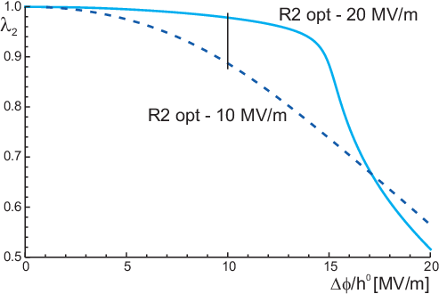
The optimum rank-two laminate layouts for the composite no. 2 are collected in Tab. 6 for both plane strain and three-dimensional traction-free problems (optimisation of $\lambda_{\rm max}$). Guided by the study of rank-one laminates by Gei et al. [9], we have selected, at an initial stage, 20 MV/m as the maximum applied nominal electric field. For this level of electric excitation, it is confirmed that the most effective microstructure arrangement corresponds to the one where the soft shell has a relatively low volume fraction (equal to 0.056 in plane strain and to 0.043 in 3D), while the two phases are almost equi-distributed in the sub rank-one core. In plane strain, the optimum $\theta_{\rm co}$ is very close to the right angle and the actuation is accompanied by a large shear strain. The plots in Fig. 7 show that the obtained rank two displays an actuation strain that is 6.6 times higher than that of the homogeneous actuator without reinforcement, while the associated optimum rank one only slightly outperforms the homogeneous response. Also for the composite no. 2, it is possible to track the change in angles $\theta_{\rm co}$ and $\theta_{\rm sh}$ along the electro-mechanical actuation path. For the plane strain case, the evolution of the angles is quite smooth; $\theta_{\rm co}$ will reduce from 88^∘ to 40^∘ at 20 MV/m, while $\theta_{\rm sh}$ will decrease from 14^∘ to about 4^∘. The set of current electric fields in the composite at $E^{0}=20$ MV/m is represented in Fig. 4b. That in the soft shell reaches 325.6 MV/m, with an amplification factor of approximately 9.3 with respect to the intensity of the overall average electric field ($E$) experienced by the composite, whose value is 34.9 MV/m.

Fig. 7 also shows the performance of an actuator optimised at a working nominal electric field of 10 MV/m whose layout information are listed in Tab. 6. At this electric field, the device under investigation clearly outclasses that optimised for 20 MV/m, being the longitudinal strain of the former more than three times larger than that of the latter. This feature obviously reverses at 20 MV/m.

These computations show the importance of the chosen working electric field for the optimisation of the composite layout. For 20 MV/m, in the three-dimensional case, the two initial layering angles are quite different than those computed in plane strain. The reason is that, differently from composite no. 1, the out-of-plane strain is now not negligibly small, then the two studied boundary-value problems lead to different layouts. On the contrary, for 10 MV/m the two configurations are very similar as at this nominal electric field the stretch $\lambda_{3}$ is very close to 1 in 3D case.

Fig. 8 reports the three stretches along actuation for the two three-dimensional problems. It can be noticed that the response of the actuator, for that optimised at 20 MV/m, is very poor up to the value $E^{0}\approx 14.5$ MV/m, beyond which the system becomes suddenly very compliant. The same trend is followed by the angles $\theta_{\rm co}$ and $\theta_{\rm sh}$: they remain almost constant up to $E^{0}\approx 14.5$ MV/m and then change quickly to reach respectively the values of 24.9^∘ and $-9.8^{\circ}$. For the layout optimised at $E^{0}=$ 10 MV/m, the increase in actuation is smoother and more similar to a parabolic function.

The problem of actuation optimisation of hierarchical rank-two dielectric elastomer composites is tackled in the non-linear electro-elasticity framework for both plane strain and three-dimensional traction free boundary-value problems. The results complement and extend those reported for small-strain computations by Tian et al. [7].

Two types of composites are considered: one is that adopted by Tian et al. [7], characterised by a matrix whose electro-mechanical properties match those of a polyurethane, for which the authors analysed configurations with equal contrast between shear moduli and electric permittivities; the other possesses a softer, silicone-like matrix, reinforced with a phase which may correspond to a poly(vinylidene fluoride) electrostrictive polymer [16].

The following conclusions can be drawn from this study.

The non-linear framework allows a better estimation of the optimum layouts of the composite that deform typically at large strains. For the former type of composite, the trend of the actuation enhancement with contrast follows a similar rule to that highlighted in [7], however the performance obtained with the non-linear model is, on average, 18% higher than that predicted at small strains. As far as the volume fractions are concerned, that of the soft phase in the inner sub rank-one core remains approximately about 0.5, independently of the value of the contrast parameter. For all the analysed cases, the optimum composite possesses a very limited volume fraction of the soft shell material (in the order of a few percents) where the electric field reaches an intensity that is one order of magnitude higher than the macroscopic counterpart in the actuator.

As a measure of the effect of the nonlinear electro-mechanical coupling, it is also demonstrated that the optimum configurations strongly depend on the maximum operational electric field chosen for the actuator. The softer is the matrix, the more observable is the phenomenon.

Acknowledgements. Support from the EU FP7 project ERC-AdG-340561-Instabilities is gratefully acknowledged.

The strain energy proposed in [12] to describe the electroelastic rank-one laminate response of the core relies on the following set of invariants:

$$I_{1}=\mbox{\boldmath${\it F}$}_{\rm co}\mbox{\boldmath$\,\cdot\,$}\mbox{\boldmath${\it F}$}_{\rm co},\ \ \ I_{2}=\mbox{\boldmath${\it F}$}_{\rm co}^{-T}\mbox{\boldmath$\,\cdot\,$}\mbox{\boldmath${\it F}$}_{\rm co}^{-T},\ \ \ I_{4}=\mbox{\boldmath${\it F}$}_{\rm co}\mbox{\boldmath${\it n}$}^{0}_{\rm co}\mbox{\boldmath$\,\cdot\,$}\mbox{\boldmath${\it F}$}_{\rm co}\mbox{\boldmath${\it n}$}^{0}_{\rm co},$$

$$I_{5}=\mbox{\boldmath${\it C}$}_{\rm co}\mbox{\boldmath${\it n}$}^{0}_{\rm co}\mbox{\boldmath$\,\cdot\,$}\mbox{\boldmath${\it C}$}_{\rm co}\mbox{\boldmath${\it n}$}^{0}_{\rm co},\ \ \ J_{7}=\mbox{\boldmath${\it F}$}_{\rm co}^{-T}\mbox{\boldmath${\it E}$}^{0}_{\rm co}\mbox{\boldmath$\,\cdot\,$}\mbox{\boldmath${\it F}$}_{\rm co}^{-T}\mbox{\boldmath${\it E}$}^{0}_{\rm co},\ \ \ J_{10}=\mbox{\boldmath${\it F}$}_{\rm co}^{-T}\mbox{\boldmath${\it E}$}_{\rm co}^{0}\mbox{\boldmath$\,\cdot\,$}\mbox{\boldmath${\it F}$}_{\rm co}^{-T}\mbox{\boldmath${\it n}$}^{0}_{\rm co},$$

(15)

where $\mbox{\boldmath${\it C}$}_{\rm co}=\mbox{\boldmath${\it F}$}_{\rm co}^{T}\mbox{\boldmath${\it F}$}_{\rm co}$. Its expression is given by

$$W_{\rm co}=\frac{\bar{\mu}}{2}(I_{1}-3)-\frac{\bar{\mu}-\tilde{\mu}}{2}\left(I_{4}-\frac{1}{I_{2}-I_{1}I_{4}+I_{5}}\right)-\frac{\bar{\varepsilon}}{2}J_{7}+\frac{\bar{\varepsilon}-\tilde{\varepsilon}}{2}\frac{J_{10}^{2}}{I_{2}-I_{1}I_{4}+I_{5}},$$

(16)

where a superposed bar signifies arithmetic average, namely $\bar{f}=c^{\rm co}_{a}f_{a}+c^{\rm co}_{b}f_{b}$, while $\tilde{f}^{-1}=c^{\rm co}_{a}/f_{a}+c^{\rm co}_{b}/f_{b}$.

References

- [1] Dorfmann, A., Ogden, R.W., 2005, Nonlinear electroelasticity, Acta Mech. 174, 167–183.
- [2] McMeeking, R.M., Landis, C.M., 2005, Electrostatic forces and stored energy for deformable dielectric materials, J. Appl. Mech., Trans. ASME 72, 581–590.
- [3] deBotton, G., Tevet-Deree, L., Socolsky, E.A., 2007, Electroactive heterogeneous polymers: analysis and applications to laminated composites, Mech. Adv. Mat. Struct. 14, 13–22.
- [4] Bertoldi, K., Gei, M., 2011, Instability in multilayered soft dielectrics, J. Mech. Phys. Solids 59, 18–42.
- [5] Rudykh, S., deBotton, G., 2011, Stability of anisotropic electroactive polymers with application to layered media, ZAMP 62, 1131–1142.
- [6] Ponte Castañeda, P., Siboni, M.N., 2012, A finite-strain constitutive theory for electroactive polymer composites via homogenization, Int. J. Nonlinear Mech. 47, 293–306.
- [7] Tian, L., Tevet–Deree, L., deBotton, G. and Bhattacharya, K., 2012, Dielectric elastomer composites, J. Mech. Phys. Solids 60, 181–198.
- [8] Rudykh, S., Lewinstein, A., Uner, G., deBotton, G., 2013, Analysis of microstructural induced enhancement of electromechanical coupling in soft dielectrics, Applied Physics Letters 102, 151905
- [9] Gei, M., Springhetti, R., Bortot, E., 2013, Performance of soft dielectric laminated composites, Smart Mater. Struct. 22, 104014.
- [10] Rudykh, S., Bhattacharya, K., DeBotton, G., 2014, Multiscale instabilities in soft heterogeneous dielectric elastomers, Proc. of the Royal Society A 470, 20130618.
- [11] Lopez-Pamies, O., 2014, Elastic dielectric composites: theory and application to particle-filled ideal dielectrics, J. Mech. Phys. Solids 64, 61–82.
- [12] Spinelli, S.A., Lopez-Pamies, O., 2015, Some simple explicit results for the elastic dielectric propertes and stability of layered composites. Int. J. Eng. Sci. 88, 15–28.
- [13] Lefevre, V., Lopez-Pamies, O., 2017, Nonlinear electroelastic deformations of dielectric elastomer composites: I–Ideal elastic dielectrics, J. Mech. Phys. Solids 99, 409–437.
- [14] Bortot, E., 2017, Analysis of multilayer electro-active spherical balloons. J. Mech. Phys. Solids 101, 250–267.
- [15] deBotton, G., 2005, Transversely isotropic sequentially laminated composites in finite elasticity. J. Mech. Phys. Solids 53, 1334–-1361.
- [16] Choi, W., Choi, K., Yang, G., Kim, J.C., Yu, C., 2016, Improving piezoelectric performance of lead-free polymer composites with high aspect ratio BaTiO3 nanowires, Polymer Testing 53, 143–148.