Mirror curve of orbifold Hurwitz numbersThanks: The first author is supported by NSF grant DMS1802082.
Abstract.
Edge-contraction operations form an effective tool in various graph enumeration problems, such as counting Grothendieck’s dessins d’enfants and simple and double Hurwitz numbers. These counting problems can be solved by a mechanism known as topological recursion, which is a mirror B-model corresponding to these counting problems. We show that for the case of orbifold Hurwitz numbers, the mirror objects, i.e., the spectral curve and the differential forms on it, are constructed solely from the edge-contraction operations of the counting problem in genus and one marked point. This forms a parallelism with Gromov-Witten theory, where genus Gromov-Witten invariants correspond to mirror B-model holomorphic geometry.
Key words and phrases:
Topological recursion; ribbon graphs; Hurwitz numbers; mirror curves2010 Mathematics Subject Classification
Primary: 14N35, 81T45, 14N10; Secondary: 53D37, 05A151. Introduction
The purpose of the present paper is to identify the mirror B-model objects that enable us to solve certain graph enumeration problems. We consider simple and orbifold Hurwitz numbers, by giving a graph enumeration formulation for these numbers. We then show that the mirror of these counting problems are constructed from the edge-contraction operations of [8] applied to orbifold Hurwitz numbers for the case of genus and one-marked point.
Edge-contraction operations provide an effective method for graph enumeration problems. It has been noted in [10] that the Laplace transform of edge-contraction operations on many counting problems corresponds to the topological recursion of [13]. In this paper, we examine the construction of mirror B-models corresponding to the simple and orbifold Hurwitz numbers. In general, enumerative geometry problems, such as computation of Gromov-Witten type invariants, are often solved by studying a corresponding problem on the mirror dual side. The effectiveness of the mirror method relies on complex analysis and holomorphic geometry technique that is available on the mirror B-model side. The question we consider in this paper is the following:
Question 1.1.
How do we find the mirror of a given enumerative problem?
We give an answer to this question for a class of graph enumeration problems that are equivalent to counting orbifold Hurwitz numbers. The key is the edge-contraction operations. The base case, or the case for the “moduli space” , of the edge contraction in the counting problem identifies the mirror dual object, and a universal mechanism of complex analysis, known as the topological recursion of [13], solves the B-model side of the counting problem. The solution is a collection of generating functions of the original counting problem for all genera.
Bouchard and Mariño [3] conjectured that generating functions for simple Hurwitz numbers could be calculated by the topological recursion of [13], based on the spectral curve identified as the Lambert curve
| (1.1) |
Here, the notion of spectral curve is the mirror dual object for the counting problem. They arrived at the mirror dual by a consideration of mirror symmetry of open Gromov-Witten invariants of toric Calabi-Yau threefolds [2]. The mirror geometry of a toric Calabi-Yau threefold is completely determined by a plane algebraic curve known as the mirror curve. The Lambert curve (1.1) appears as the infinite framing number limit of the mirror curve of . The Hurwitz number conjecture of [3] was then solved in a series of papers by one of the authors [12, 20], using the Lambert curve as a given input. Since conjecture is true, the Lambert curve (1.1) should be the mirror B-model for Hurwitz numbers. But why? In [12, 20], we did not attempt to give any explanation.
The emphasis of our current paper is to prove that the mirror dual object is simply a consequence of the case of the edge-contraction operation on the original counting problem. The situation is similar to several cases of Gromov-Witten theory, where the mirror is constructed by the genus Gromov-Witten invariants themselves.
To illustrate the idea, let us consider the number of connected trees consisting of labeled nodes (or vertices). The initial condition is . The numbers satisfy a recursion relation
| (1.2) |
A tree of nodes has edges. The left-hand side counts how many ways we can eliminate an edge. When an edge is eliminated, the tree breaks down into two disjoint pieces, one consisting of labeled nodes, and the other labeled nodes. The original tree is restored by connecting one of the nodes on one side to one of the nodes on the other side. The equivalence of counting in this elimination process gives (1.2). From the initial value, the recursion formula generates the tree sequence . We note, however, that (1.2) does not directly give a closed formula for . To find one, we introduce a generating function, or a spectral curve
| (1.3) |
In terms of the generating function, (1.2) becomes equivalent to
| (1.4) |
The initial condition is and , which allows us to solve the differential equation uniquely. Lo and behold, the solution is exactly (1.1).
To find the formula for , we need the Lagrange Inversion Formula. Suppose that is a holomorphic function defined near , and that . Then the inverse function of near is given by
| (1.5) |
The proof is elementary and requires only Cauchy’s integration formula. Since in our case, we immediately obtain Cayley’s formula .
The point we wish to make here is that the real problem behind the scene is not tree-counting, but simple Hurwitz numbers. This relation is understood by the correspondence between trees and ramified coverings of by of degree that are simply ramified except for one total ramification point. When we look at the dual graph of a tree, elimination of an edge becomes contracting an edge, and this operation precisely gives a degeneration formula for counting problems on . The base case for the counting problem is , and the recursion (1.2) is the result of the edge-contraction operation for simple Hurwitz numbers associated with . In this sense, the Lambert curve (1.1) is the mirror dual of simple Hurwitz numbers.
The paper is organized as follows. In Section 2, we present combinatorial graph enumeration problems, and show that they are equivalent to counting of simple and orbifold Hurwitz numbers. In Section 3, the spectral curves of the topological recursion for simple and orbifold Hurwitz numbers (the mirror objects to the counting problems) are constructed from the edge-contraction formulas for invariants.
2. Orbifold Hurwitz numbers as graph enumeration
Mirror symmetry provides an effective tool for counting problems of Gromov-Witten type invariants. The question is how we construct the mirror, given a counting problem. Although there is so far no general formalism, we present a systematic procedure for computing orbifold Hurwitz numbers in this paper. The key observation is that the edge-contraction operations for identify the mirror object.
The topological recursion for simple and orbifold Hurwitz numbers are derived as the Laplace transform of the cut-and-join equation [1, 12, 20], where the spectral curves are identified by the consideration of mirror symmetry of toric Calabi-Yau orbifolds [1, 3, 14, 15]. In this section we give a purely combinatorial graph enumeration problem that is equivalent to counting orbifold Hurwitz numbers. We then show in the next section that the edge-contraction formula restricted to the case determines the spectral curve and the differential forms and of [1]. These quantities form the mirror objects for the orbifold Hurwitz numbers.
2.1. Cell graphs
To avoid unnecessary confusion, we use the terminology cell graphs in this article, instead of more common ribbon graphs. Ribbon graphs naturally appear for encoding complex structures of a topological surface (see for example, [17, 18]). Our purpose of using ribbon graphs are for degeneration of stable curves, and we label vertices, instead of faces, of a ribbon graph.
Definition 2.1 (Cell graphs).
A connected cell graph of topological type is the -skeleton of a cell-decomposition of a connected closed oriented surface of genus with labeled -cells. We call a -cell a vertex, a -cell an edge, and a -cell a face, of the cell graph. We denote by the set of connected cell graphs of type . Each edge consists of two half-edges connected at the midpoint of the edge.
Remark 2.2.
- •
The dual of a cell graph is a ribbon graph, or Grothendieck’s dessin d’enfant. We note that we label vertices of a cell graph, which corresponds to face labeling of a ribbon graph. Ribbon graphs are also called by different names, such as embedded graphs and maps.
- •
We identify two cell graphs if there is a homeomorphism of the surfaces that brings one cell-decomposition to the other, keeping the labeling of -cells. The only possible automorphisms of a cell graph come from cyclic rotations of half-edges at each vertex.
Definition 2.3 (Directed cell graph).
A directed cell graph is a cell graph for which an arrow is assigned to each edge. An arrow is the same as an ordering of the two half-edges forming an edge. The set of directed cell graphs of type is denoted by .
Remark 2.4.
A directed cell graph is a quiver. Since our graph is drawn on an oriented surface, a directed cell graph carries more information than its underlying quiver structure. The tail vertex of an arrowed edge is called the source, and the head of the arrow the target, in the quiver language.
An effective tool in graph enumeration is edge-contraction operations. Often edge contraction leads to an inductive formula for counting problems of graphs.
Definition 2.5 (Edge-contraction operations).
There are two types of edge-contraction operations applied to cell graphs.
- •
ECO 1: Suppose there is a directed edge in a cell graph , connecting the tail vertex and the head vertex . We contract in , and put the two vertices and together. We use for the label of this new vertex, and call it again . Then we have a new cell graph with one less vertices. In this process, the topology of the surface on which is drawn does not change. Thus genus of the graph stays the same.
Figure 2.1. Edge-contraction operation ECO 1. The edge bounded by two vertices and is contracted to a single vertex . - •
We use the notation for the edge-contraction operation
(2.1) - •
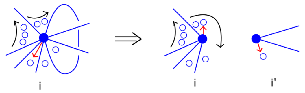
ECO 2: Suppose there is a directed loop in at the -th vertex . Since a loop in the -skeleton of a cell decomposition is a topological cycle on the surface, its contraction inevitably changes the topology of the surface. First we look at the half-edges incident to vertex . Locally around on the surface, the directed loop separates the neighborhood of into two pieces. Accordingly, we put the incident half-edges into two groups. We then break the vertex into two vertices, and , so that one group of half-edges are incident to , and the other group to . The order of two vertices is determined by placing the loop upward near at vertex . Then we name the new vertex on its left by , and on its right by .
Let denote the possibly disconnected graph obtained by contracting and separating the vertex to two distinct vertices labeled by and .
Figure 2.2. Edge-contraction operation ECO 2. The contracted edge is a loop of a cell graph. Place the loop so that it is upward near at to which is attached. The vertex is then broken into two vertices, on the left, and on the right. Half-edges incident to are separated into two groups, belonging to two sides of the loop near . - •
If is connected, then it is in . The loop is a loop of handle. We use the same notation to indicate the edge-contraction operation
(2.2) - •
If is disconnected, then write , where
(2.3) The edge-contraction operation is again denoted by
(2.4) In this case we call a separating loop. Here, vertices labeled by belong to the connected component of genus , and those labeled by are on the other component of genus . Let (reps. ) be the reordering of (resp. ) in the increasing order. Although we give labeling to the two vertices created by breaking , since they belong to distinct graphs, we can simply use for the label of and the same for . The arrow of translates into the information of ordering among the two vertices and .
Remark 2.6.
The use of directed cell graphs enables us to define edge-contraction operations, keeping track with vertex labeling. We refer to [OM6] for the actual motivation for quiver cell graphs. Since our main concern is enumeration of graphs, the extra data of directed edges does not plan any role. In what follows, we deal with cell graphs without directed edges. The edge-contraction operations are defined with a choice of direction, but the counting formula we derive does not depend of this choice.
Remark 2.7.
Let us define for a graph . Then every edge-contraction operation reduces exactly by . Indeed, for ECO 1, we have
The ECO 2 applied to a loop of handle produces
For a separating loop, we have
2.2. -Hurwitz graphs
We choose and fix a positive integer . The decorated graphs we wish to enumerate are the following.
Definition 2.8 (-Hurwitz graph).
An -Hurwitz graph of type consists of the following data.
- •
is a connected cell graph of type , with labeled vertices.
- •
is divisible by , and has unlabeled faces and unlabeled edges, where
(2.5) - •
is a configuration of unlabeled dots on the graph subject to the following conditions:
- (1)
The set of dots are grouped into subsets of dots, each of which is equipped with a cyclic order.
- (2)
Every face of has cyclically ordered dots.
- (3)
These dots are clustered near vertices of the face. At each corner of the face, say at Vertex , the dots are ordered according to the cyclic order that is consistent of the orientation of the face, which is chosen to be counter-clock wise.
- (4)
Let denote the total number of dots clustered at Vertex . Then for every . Thus we have an ordered partition
(2.6) In particular, the number of vertices ranges .
- (5)
Suppose an edge connecting two distinct vertices, say Vertex and , bounds the same face twice. Let be the midpoint of . The polygon representing the face has twice on its perimeter, hence the point appears also twice. We name them as and . Which one we call or does not matter. Consider a path on the perimeter of this polygon starting from and ending up with according to the counter-clock wise orientation. Let be the total number of dots clustered around vertices of the face, counted along the path. Then it satisfies
(2.7) For example, not all dots of a face can be clustered at a vertex of degree . In particular, for the case of , the graph has no edges bounding the same face twice.
- (1)
An arrowed -Hurwitz graph has, in addition to to the above data , an arrow assigned to one of the dots from Vertex for each index .
The counting problem we wish to study is the number of arrowed -Hurwitz graphs for a prescribed ordered partition (2.6), counted with the automorphism weight. The combinatorial data corresponds to an object in algebraic geometry. Let us first identify what the -Hurwitz graphs represent. We denote by the -dimensional orbifold modeled on that has one stacky point at .
Example 2.9.
The base case is (see Figure 2.3). This counts the identity morphism .

Definition 2.10 (Orbifold Hurwitz cover and Orbifold Hurwitz numbers).
An orbifold Hurwitz cover is a morphism from an orbifold that is modeled on a smooth algebraic curve of genus that has
- (1)
stacky points of the same type as the one on the base curve that are all mapped to ,
- (2)
arbitrary profile with labeled points over ,
- (3)
and all other ramification points are simple.
If we replace the target orbifold by , then the morphism is a regular map from a smooth curve of genus with profile over , labeled profile over , and a simple ramification at any other ramification point. The Euler characteristic condition (2.5) of the graph gives the number of simple ramification points of through the Riemann-Hurwitz formula. The automorphism weighted count of the number of the topological types of such covers is denoted by . These numbers are referred to as orbifold Hurwitz numbers. When , they count the usual simple Hurwitz numbers.
The counting of the topological types is the same as counting actual orbifold Hurwitz covers such that all simple ramification points are mapped to one of the -th roots of unity , where , if all simple ramification points of are labeled. Indeed, such a labeling is given by elements of the cyclic group of order . Let us construct an edge-labeled Hurwitz graph from an orbifold Hurwitz cover with fixed branch points on the target as above. We first review the case of , i.e., the simple Hurwitz covers. Our graph is essentially the same as the dual of the branching graph of [21].
2.3. Construction of -Hurwitz graphs
First we consider the case . Let be a simple Hurwitz cover of genus and degree with labeled profile over , unramified over , and simply ramified over , where and . We denote by the labeled simple ramification points of , that is bijectively mapped to by . We choose a labeling of so that for every .
On , plot and connect each element with by a straight line segment. We also connect and by a straight line , . Let denote the configuration of the line segments. The inverse image is a cell graph on , for which forms the set of vertices. We remove all inverse images of the line segment from this graph, except for the ones that end at one of the points . Since is a simple ramification point of , the line segment ending at extends to another vertex, i.e., another point in . We denote by the graph after this removal of line segments. We define the edges of the graph to be the connected line segments at for some . We use as the label of the edge. The graph has vertices, edges, and faces.
An inverse image of the line is a ray starting at a vertex of the graph and ending up with one of the points in , which is the center of a face. We place a dot on this line near at each vertex. The edges of incident to a vertex are cyclically ordered counter-clockwise, following the natural cyclic order of . Let be an edge incident to a vertex, and the next one at the same vertex according to the cyclic order. We denote by the number of dots in the span of two edges and , which is if , and if . Now we consider the dual graph of . It has vertices, faces, and edges still labeled by . At the angled corner between the two adjacent edges labeled by and in this order according to the cyclic order, we place dots. The data consisting of the cell graph and the dot configuration is the Hurwitz graph corresponding to the simple Hurwitz cover for .
It is obvious that what we obtain is an Hurwitz graph, except for the condition (5) of the configuration , which requires an explanation. The dual graph for is the branching graph of [21]. Since is the number of simple ramification points, which is also the number of edges of , the branching graph cannot have any loops. This is because two distinct powers of in the range of cannot be the same. This fact reflects in the condition that has no edge that bounds the same face twice. This explains the condition (5) for .
Remark 2.11.
If we consider the case and , then . Hence the graph is a connected tree consisting of nodes (vertices) and labeled edges. Except for , every vertex is uniquely labeled by incident edges. The tree counting of Introduction is relevant to Hurwitz numbers in this way.
Now let us consider an orbifold Hurwitz cover of genus and degree with labeled profile over , isomorphic stacky points over , and simply ramified over , where . By we indicate the labeled simple ramification points of , that is again bijectively mapped to by . We choose the same labeling of so that for every .
On , plot and connect each element with the stacky point at by a straight line segment. We also connect and by a straight line , , as before. Let denote the configuration of the line segments. The inverse image is a cell graph on , for which forms the set of vertices. We remove all inverse images of the line segment from this graph, except for the ones that end at one of the points . We denote by the graph after this removal of line segments. We define the edges of the graph to be the connected line segments at for some . We use as the label of the edge. The graph has vertices, edges.
The inverse image of the line form a set of rays at each vertex of the graph , connecting vertices and centers of faces. We place a dot on each line near at each vertex. These dots are cyclically ordered according to the orientation of , which we choose to be counter-clock wise. The edges of incident to a vertex are also cyclically ordered in the same way. Let be an edge incident to this vertex, and the next one according to the cyclic order. We denote by the number of dots in the span of two edges and . Let denote the dual graph of . It now has vertices, faces, and edges still labeled by . At the angled corner between the two adjacent edges labeled by and in this order according to the cyclic order, we place dots, again cyclically ordered as on . The data consisting of the cell graph and the dot configuration is the -Hurwitz graph corresponding to the orbifold Hurwitz cover .
We note that can have loops, unlike the case of . Let us place locally on an oriented plane around a vertex. The plane is locally separated into sectors by the rays at this vertex. There are half-edges coming out of the vertex at each of these sectors. A half-edge corresponding to cannot be connected to another half-edge corresponding to in the same sector, by the same reason for the case of . But it can be connected to another half-edge of a different sector corresponding again to the same . In this case, within the loop there are some dots, representing the rays of in between these half-edges. The total number of dots in the loop cannot be , because then the half-edges being connected are in the same sector. Thus the condition (5) is satisfied.
Example 2.12.
Theorem 2.15 below shows that
This is the weighted count of the number of -Hurwitz graphs of type with an ordered partition .


In terms of formulas, the -Hurwitz cover corresponding to the graph on the left of Figure 2.5 is given by
To make the simple ramification points sit on , we need to divide by , where are the simple ramification points. The -Hurwitz cover corresponding to the graph on the right of Figure 2.5 is given by
where is a real number satisfying . The real parameter changes the topological type of the -Hurwitz cover. For , the graph is the same as on the left, and for , the graph becomes the one on the right.
2.4. The edge-contraction formulas
Definition 2.13 (Edge-contraction operations).
The edge-contraction operations (ECOs) on an arrowed -Hurwitz graph are the following procedures. Choose an edge of the cell graph .
- •
ECO 1: We consider the case that is an edge connecting two distinct vertices Vertex and Vertex . We can assume , which induces a direction on . Let us denote by and the faces bounded by , where is on the left side of with respect to the direction. We now contract , with the following additional operations:
- (1)
Remove the original arrows at Vertices and .
- (2)
Put the dots on clustered at Vertices and together, keeping the cyclic order of the dots on each of .
- (3)
Place a new arrow to the largest dot on the corner at Vertex of Face with respect to the cyclic order.
- (4)
If there are no dots on this particular corner, then place an arrow to the first dot we encounter according to the counter-clock wise rotation from and centered at Vertex .
- (1)
The new arrow at the joined vertex allows us to recover the original graph from the new one.

- •
ECO 2: This time is a loop incident to Vertex twice. We contract and separate the vertex into two new ones, as in ECA 3 of Definition . The additional operations are:
- (1)
The contraction of a loop does not change the number of faces. Separate the dots clustered at Vertex according to the original configuration.
- (2)
Look at the new vertex to which the original arrow is placed. We keep the same name to this vertex. The other vertex is named .
- (3)
Place a new arrow to the dot on the corner at the new Vertex that was the largest in the original corner with respect to the cyclic order.
- (4)
If there are no dots on this particular corner, then place an arrow to the first dot we encounter according to the counter-clock wise rotation from and centered at Vertex on the side of the old arrow.
- (5)
We do the same operation for the new Vertex , and put a new arrow to a dot.
- (6)
Now remove the original arrow.
- (1)
Although cumbersome, it is easy to show that
Lemma 2.14.
The edge-contraction operations preserve the set of -Hurwitz graphs.
An application of the edge-contraction operations is the following counting recursion formula.
Theorem 2.15 (Edge-Contraction Formula).
The number of arrowed Hurwitz graphs satisfy the following edge-contraction formula.
| (2.8) | ||||
Here, indicates the omission of the index, and for any subset .
Remark 2.16.
The edge-contraction formula (ECF) is a recursion with respect to the number of edges
Therefore, it calculates all values of from the base case . However, it does not determine the initial value itself, since . We also note that the recursion is not for as a function in integer variables.
Proof.
The counting is done by applying the edge-contraction operations. The left-hand side of (2.8) shows the choice of an edge, say , out of edges. The first line of the right-hand side corresponds to the case that the chosen edge connects Vertex and Vertex . We assume , and apply ECO 1. The factor indicates the removal of two arrows at these vertices (Figure 2.6).
When the edge we have chosen is a loop incident to Vertex twice, then we apply ECO 2. The factor is the removal of the original arrow (Figure 2.7). The second and third lines on the right-hand side correspond whether is a handle-cutting loop, or a separation loop. The factor is there because of the symmetry between and of the partition of . This complete the proof. ∎
Theorem 2.17 (Graph enumeration and orbifold Hurwitz numbers).
The graph enumeration and counting orbifold Hurwitz number are related by the following formula:
| (2.9) |
Proof.
The simplest orbifold Hurwitz number is , which counts double Hurwitz numbers with the same profile at both and . There is only one such map , which is given by . Since the map has automorphism , we have . Thus (2.9) holds for the base case.
3. Construction of the mirror spectral curves for orbifold Hurwitz numbers
In the earlier work on simple and orbifold Hurwitz numbers in connection to the topological recursion [1, 3, 5, 12, 20], the spectral curves are determined by the infinite framing limit of the mirror curves to toric Calabi-Yau (orbi-)threefolds. The other ingredients of the topological recursion, the differential forms and , are calculated by the Laplace transform of the and cases of the ELSV [11] and JPT [16] formulas. Certainly the logic is clear, but why these choices are the right ones is not well explained.
In this section, we show that the edge-contraction operations themselves determine all the mirror ingredients, i.e., the spectral curve, , and . The structure of the story is the following. The edge-contraction formula (2.8) is an equation among different values of . When restricted to , it produces an equation on as a function in one integer variable. The generating function of is reasonably complicated, but it can be expressed rather nicely in terms of the generating function of the -values , which is essentially the spectral curve of the theory. The edge-contraction formula (2.8) itself has the Laplace transform that can be calculated in the spectral curve coordinate. Since (2.8) contains on each side of the equation, to make it a genuine recursion formula for functions with respect to in the stable range, we need to calculate the generating functions of and , and make the rest of (2.8) free of unstable terms. The result is the topological recursion of [1, 12].
Let us now start with the restricted (2.8) on invariants:
| (3.1) |
At this stage, we introduce a generating function
| (3.2) |
In terms of this generating function, (3.1) is a differential equation
| (3.3) |
or simply
Its unique solution is
with a constant of integration . As we noted in the previous section, the recursion (2.8) does not determine the initial value . For our graph enumeration problem, the values are
| (3.4) |
which determine . Thus we find
| (3.5) |
which is the -Lambert curve of [1]. This is indeed the spectral curve for the orbifold Hurwitz numbers.
Remark 3.1.
We note that satisfies the same recursion equation (3.1) for , with a different initial value. Thus essentially orbifold Hurwitz numbers are determined by the usual simple Hurwitz numbers.
Remark 3.2.
For the purpose of performing analysis on the spectral curve (3.5), let us introduce a global coordinate on the -Lambert curve, which is an analytic curve of genus :
| (3.6) |
We denote by this parametric curve. Let us introduce the generating functions of general , which are called free energies:
| (3.7) |
We also define the exterior derivative
| (3.8) |
which is a symmetric -linear differential form. By definition, we have
| (3.9) |
The topological recursion requires the spectral curve, , and . From (3.8) and (3.9), we have
| (3.10) |
Remark 3.3.
As a differential equation, we can solve (3.9) in a closed formula on the spectral curve of (3.6). Indeed, the role of the spectral curve is that the free energies, i.e., ’s, are actually analytic functions defined on . Although we define ’s as a formal power series in as generating functions, they are analytic, and the domain of analyticity, or the classical sense of Riemann surface, is the spectral curve . The coordinate change (3.6) gives us
| (3.11) |
hence (3.9) is equivalent to
Since , we find
| (3.12) |
The calculation of is done similarly, by restricting (2.8) to the and terms. Assuming that , we have
| (3.13) |
As a special case of [1, Lemma 4.1], this equation translates into a differential equation for :
| (3.14) |
Denoting by and using (3.11), (3.14) becomes simply
| (3.15) |
on the spectral curve . This is a linear partial differential equation of the first order with analytic coefficients in the neighborhood of , hence by the Cauchy-Kovalevskaya theorem, it has the unique analytic solution around the origin of for any Cauchy problem. Since the only analytic solution to the homogeneous equation
is a constant, the initial condition determines the unique solution of (3.15).
Proposition 3.4.
We have a closed formula for in the -coordinates:
| (3.16) |
Proof.
In [1], the functions (3.12) and (3.16) are derived by directly computing the Laplace transform of the JPT formulas [16]
| (3.17) | ||||
Here, gives the decomposition of a rational number into its floor and the fractional part. We have thus recovered (3.17) from the edge-contraction formula alone, which are the and cases of the ELSV formula for the orbifold Hurwitz numbers.
Acknowledgement.
The paper is based a series of lectures by M.M. at Mathematische Arbeitstagung 2015, Max-Planck-Institut für Mathematik in Bonn. The authors are grateful to the American Institute of Mathematics in California, the Banff International Research Station, the Institute for Mathematical Sciences at the National University of Singapore, Kobe University, Leibniz Universität Hannover, the Lorentz Center for Mathematical Sciences, Leiden, Max-Planck-Institut für Mathematik in Bonn, and Institut Henri Poincaré, Paris, for their hospitality and financial support during the authors’ stay for collaboration. The research of O.D. has been supported by GRK 1463 Analysis, Geometry, and String Theory at Leibniz Universität Hannover and MPIM. The research of M.M. has been supported by NSF grants DMS-1309298, DMS-1619760, DMS-1642515, and NSF-RNMS: Geometric Structures And Representation Varieties (GEAR Network, DMS-1107452, 1107263, 1107367).
References
- [1] V. Bouchard, D. Hernández Serrano, X. Liu, and M. Mulase, Mirror symmetry for orbifold Hurwitz numbers, arXiv:1301.4871 [math.AG] (2013).
- [2] V. Bouchard, A. Klemm, M. Mariño, and S. Pasquetti, Remodeling the B-model, Commun. Math. Phys. 287, 117–178 (2009).
- [3] V. Bouchard and M. Mariño, Hurwitz numbers, matrix models and enumerative geometry, Proc. Symposia Pure Math. 78, 263–283 (2008).
- [4] R. Dijkgraaf, E. Verlinde, and H. Verlinde, Loop equations and Virasoro constraints in non-perturbative two-dimensional quantum gravity, Nucl. Phys. B348, 435–456 (1991).
- [5] N. Do, O. Leigh, and P. Norbury, Orbifold Hurwitz numbers and Eynard-Orantin invariants, arXiv:1212.6850 (2012).
- [6] O. Dumitrescu and M. Mulase, Quantum curves for Hitchin fibrations and the Eynard-Orantin theory, Lett. Math. Phys. 104, 635–671 (2014).
- [7] O. Dumitrescu and M. Mulase, Quantization of spectral curves for meromorphic Higgs bundles through topological recursion, arXiv:1411.1023 (2014).
- [8] O. Dumitrescu and M. Mulase, Edge contraction on dual ribbon graphs and 2D TQFT, Journal of Algebra, vol. 494, January 2018.
- [9] O. Dumitrescu and M. Mulase, Lectures on the topological recursion for Higgs bundles and quantum curves, to appear in the lecture notes series of the National University of Singapore.
- [10] O. Dumitrescu, M. Mulase, A. Sorkin and B. Safnuk, The spectral curve of the Eynard-Orantin recursion via the Laplace transform, in “Algebraic and Geometric Aspects of Integrable Systems and Random Matrices,” Dzhamay, Maruno and Pierce, Eds. Contemporary Mathematics 593, 263–315 (2013).
- [11] T. Ekedahl, S. Lando, M. Shapiro, A. Vainshtein, Hurwitz numbers and intersections on moduli spaces of curves, Invent. Math. 146, 297–327 (2001) [arXiv:math/0004096].
- [12] B. Eynard, M. Mulase and B. Safnuk, The Laplace transform of the cut-and-join equation and the Bouchard-Mariño conjecture on Hurwitz numbers, Publications of the Research Institute for Mathematical Sciences 47, 629–670 (2011).
- [13] B. Eynard and N. Orantin, Invariants of algebraic curves and topological expansion, Communications in Number Theory and Physics 1, 347–452 (2007).
- [14] B. Fang, C.-C. M. Liu, and Z. Zong, All genus open-closed mirror symmetry for affine toric Calabi-Yau 3-orbifolds, arXiv:1310.4818 [math.AG] (2013).
- [15] B. Fang, C.-C. M. Liu, and Z. Zong, On the Remodeling Conjecture for Toric Calabi-Yau 3-Orbifolds, arXiv:1604.07123 (2016).
- [16] P. Johnson, R. Pandharipande, and H.H. Tseng, Abelian Hurwitz-Hodge integrals, Michigan Math. J. 60, 171–198 (2011) [arXiv:0803.0499].
- [17] M. Kontsevich, Intersection theory on the moduli space of curves and the matrix Airy function, Communications in Mathematical Physics 147, 1–23 (1992).
- [18] M. Mulase and M. Penkava, Ribbon graphs, quadratic differentials on Riemann surfaces, and algebraic curves defined over , The Asian Journal of Mathematics 2 (4), 875–920 (1998).
- [19] M. Mulase and P. Sułkowski, Spectral curves and the Schrödinger equations for the Eynard-Orantin recursion, arXiv:1210.3006 (2012).
- [20] M. Mulase and N. Zhang, Polynomial recursion formula for linear Hodge integrals, Communications in Number Theory and Physics 4, 267–294 (2010).
- [21] A. Okounkov and R. Pandharipande, Gromov-Witten theory, Hurwitz numbers, and matrix models, I, Proc. Symposia Pure Math. 80, 325–414 (2009).
- [22] C. Teleman, The structure of 2D semi-simple field theories, Inventiones Mathematicae 188, 525–588 (2012).
- [23] G. ’t Hooft, A planer diagram theory for strong interactions, Nuclear Physics B 72, 461–473 (1974).
- [24] E. Witten, Two dimensional gravity and intersection theory on moduli space, Surveys in Differential Geometry 1, 243–310 (1991).