跳到论文正文
W Papers独立论文阅读器 arXiv:1904.04774 论文正文 计算阅读时间 · 0%
引用这篇论文根据当前论文元数据生成,正式投稿前建议核对。


License: arXiv.org perpetual non-exclusive license
arXiv:1904.04774v3 [math.ST] 24 Feb 2020

Drift Estimation for Stochastic Reaction-Diffusion Systems

Gregor Pasemann and Wilhelm Stannat Address: TU Berlin, Institut für Mathematik, Str. des 17. Juni 136, D-10623 Berlin, Germany Email address: pasemann@math.tu-berlin.de Address: TU Berlin, Institut für Mathematik, Str. des 17. Juni 136, D-10623 Berlin, Germany Email address: stannat@math.tu-berlin.de
Abstract.

A parameter estimation problem for a class of semilinear stochastic evolution equations is considered. Conditions for consistency and asymptotic normality are given in terms of growth and continuity properties of the nonlinear part. Emphasis is put on the case of stochastic reaction-diffusion systems. Robustness results for statistical inference under model uncertainty are provided.

Key words and phrases: 
Parametric Drift Estimation, Robustness, Semilinear Stochastic Partial Differential Equations, Maximum Likelihood Estimation, Fitzhugh-Nagumo System

We consider a semilinear stochastic partial differential equation (SPDE)

(1) d​X​(t,x)=θ​A​X​(t,x)​d​t+F⁡(t,X⁡(t,x))​d​t+B​d​W​(t,x)\mathrm{d}X(t,x)=\theta AX(t,x)\mathrm{d}t+F(t,X(t,x))\mathrm{d}t+B\mathrm{d}W(t,x)

with X​(0,x)=X0​(x)X(0,x)=X_{0}(x) on a suitable domain 𝒟⊂ℝn\mathcal{D}\subset\mathbb{R}^{n}. Detailed conditions for the terms appearing in (1) are stated in Section 1.1. We write Xt=X⁡(t,x)X_{t}=X(t,x) for short. Assume that we are given complete information on the process XX up to a finite time T>0T>0. The statistical problem we are interested in consists in estimating the unknown value θ>0\theta>0.

To this end, we adopt a maximum likelihood based approach. Denote by XNX^{N} the NN-dimensional approximation to the solution trajectory obtained by truncation in Fourier space. XNX^{N} generates a probability measure on the space of continuous paths with values in ℝN\mathbb{R}^{N}, denoted ℙθN\mathbb{P}_{\theta}^{N}. Of course, different values for θ\theta lead to different measures on path space. We fix a reference parameter θ0>0\theta_{0}>0 (which is arbitrary and does not necessarily coincide with the true parameter) and formally apply a version of Girsanov’s theorem (as in [23], Section 7.6.4) in order to obtain a representation for the density of ℙθN\mathbb{P}^{N}_{\theta} with respect to ℙθ0N\mathbb{P}^{N}_{\theta_{0}}:

d​ℙθNd​ℙθ0N​(XN)=\displaystyle\frac{\mathrm{d}\mathbb{P}^{N}_{\theta}}{\mathrm{d}\mathbb{P}^{N}_{\theta_{0}}}(X^{N})= exp⁡((θ−θ0)​∫0T⟨A​XtN,(B​BT)−1​d​XtN⟩CLOSE\displaystyle\exp\left((\theta-\theta_{0})\int_{0}^{T}\left\langle AX^{N}_{t},(BB^{T})^{-1}\mathrm{d}X^{N}_{t}\right\rangle\right.
−12(θ2−θ02)∫0T|B−TAXtN|2dt−(θ−θ0)∫0T⟨(BBT)−1AXtN,FN(t,Xt)⟩dt).\displaystyle\left.-\frac{1}{2}(\theta^{2}-\theta_{0}^{2})\int_{0}^{T}|B^{-T}AX^{N}_{t}|^{2}\mathrm{d}t-(\theta-\theta_{0})\int_{0}^{T}\langle(BB^{T})^{-1}AX^{N}_{t},F^{N}(t,X_{t})\rangle\mathrm{d}t\right).

Here, FNF^{N} is the NN-dimensional Fourier approximation of FF. Maximizing the log-likelihood with respect to θ\theta yields the following estimator:

(2) θ^N=∫0T⟨A​XtN,(B​BT)−1​d​XtN⟩−∫0T⟨(B​BT)−1​A​XtN,FN​(t,Xt)⟩​𝑑t∫0T|B−T​A​XtN|2​𝑑t.\hat{\theta}_{N}=\frac{\int_{0}^{T}\left\langle AX^{N}_{t},(BB^{T})^{-1}\mathrm{d}X^{N}_{t}\right\rangle-\int_{0}^{T}\langle(BB^{T})^{-1}AX^{N}_{t},F^{N}(t,X_{t})\rangle\mathrm{d}t}{\int_{0}^{T}|B^{-T}AX^{N}_{t}|^{2}\mathrm{d}t}.

Note that the derivation of θ^N\hat{\theta}_{N} is purely heuristic, so asymptotic properties of the estimator cannot be simply derived from the general theory of maximum likelihood estimation (as presented e.g. in [18]).

The aim of this work is to extend the results from [9] to a class of semilinear stochastic evolution equations of the form (1). We analyze different variants of θ^N\hat{\theta}_{N}, which correspond to different ways of handling the nonlinear term, see Section 1.2 for details. All estimators are based on the Fourier decomposition of XX. We present conditions concerning growth and continuity properties of the nonlinear operator FF which are sufficient to guarantee consistency and asymptotic normality for these estimators as the number of Fourier modes NN tends to infinity (see Theorem 1.2 in Section 1.3). Special emphasis is put on the important case of stochastic reaction-diffusion systems with polynomial nonlinearities. Furthermore, we study the impact of model misspecification on estimating θ\theta in Section 2.5. More precisely: Assume that the true nonlinearity FF which governs the dynamics of XX is unknown or too complex to be handled directly. We discuss to what extent FF may be approximated by a simple model nonlinearity FapproxF^{\mathrm{approx}} from the point of view of parameter estimation. Finally, we show how to adapt the argument in order to deal with a coupled system of reaction-diffusion equations, see Section 5. Our motivation in this regard is to study conductance-based neuronal models, see [33] and references therein.

Statistical Inference, in particular drift estimation, of stochastic ordinary differential equations (SODEs) is a well-established theory, see e.g. [20, 23, 22]. It is a well-known fact that it is in general not possible to identify the drift term of an SODE in finite time. The reason is that due to Girsanov’s theorem the measures on path space generated by different drift terms are mutually equivalent. However, as T→∞T\rightarrow\infty, the true drift can be recovered asymptotically. The same is true for stochastic evolution equations with bounded drift on general function spaces.

Notably the situation changes for SPDEs with unbounded drift containing differential operators. In this case, it is usually possible to identify the coefficient in front of the leading term of the drift operator. This has been observed first in [14] and [17] (see also [15]), and since then various publications have been devoted to studying and expanding this phenomenon, see e.g. [26, 28, 16, 32] for the case of non-diagonalizable linear equations. Notice also the recent works [2] dealing with local measurements and [31, 3, 5, 6, 10, 8] for parameter estimation under spatially and temporally discrete observations for a high-frequency regime. Surveys are presented in [27, 7]. The main focus, however, has been put on linear equations such as the stochastic heat equation, which corresponds to the case that FF is either zero or another linear operator. So far, only few results about parameter estimation for nonlinear SPDEs are available, most notably [9] (see also [7]), which considers the 2D Navier–Stokes equations and serves as a guideline for our work.

1. The Model

1.1. General Form of the Equation

Throughout this work we fix a final time T>0T>0. Let HH be a Hilbert space with inner product (⋅,⋅)H(\cdot,\cdot)_{H}. Let AA be some negative definite self-adjoint operator on HH with compact resolvent and domain D⁡(A)⊂HD(A)\subset H. We write V=D⁡((−A)12)V=D((-A)^{\frac{1}{2}}). Recall that V⊂H≃H∗⊂V∗V\subset H\simeq H^{*}\subset V^{*} is a Gelfand triple, and for h∈Hh\in H and v∈Vv\in V we have ⟨h,v⟩VV∗=(h,v)H{}_{V^{*}}\langle h,v\rangle_{V}=(h,v)_{H}, where ⟨⋅,⋅⟩VV∗{}_{V^{*}}\langle\cdot,\cdot\rangle_{V} is the dual pairing between VV and its dual V∗≃D⁡((−A)−12)V^{*}\simeq D((-A)^{-\frac{1}{2}}). The general model we are interested in is given by the following equation in HH:

(3) d​Xt=(θ​A​Xt+F⁡(t,Xt))​d​t+B​d​Wt,\mathrm{d}X_{t}=(\theta AX_{t}+F(t,X_{t}))\mathrm{d}t+B\mathrm{d}W_{t},

together with initial condition X0∈HX_{0}\in H. Here, F:[0,T]×V→V∗F:[0,T]\times V\rightarrow V^{*} is a (possibly nonlinear) measurable operator, WW is a cylindrical Wiener process on HH with respect to some stochastic basis (Ω,ℱ,(ℱt)t≥0,ℙ)(\Omega,\mathcal{F},(\mathcal{F}_{t})_{t\geq 0},\mathbb{P}), and B∈L2​(H)B\in L_{2}(H) is of Hilbert–Schmidt type. As we need weak solutions only, the stochastic basis and the cylindrical Wiener process WW need not be determined in advance. The number θ>0\theta>0 is the unknown parameter to be estimated.

For simplicity, we restrict ourselves to the case B=(−A)−γB=(-A)^{-\gamma}, γ>0\gamma>0. For later use, we introduce some notations. Let (Φk)k∈ℕ⊂H(\Phi_{k})_{k\in\mathbb{N}}\subset H be an ONB of eigenvectors of −A-A such that the corresponding eigenvalues (taking into account multiplicity) (λk)k∈ℕ(\lambda_{k})_{k\in\mathbb{N}} are ordered increasingly. For N∈ℕN\in\mathbb{N}, the projection onto the span of Φ1,…,ΦN\Phi_{1},\dots,\Phi_{N} is called PN:H→span⁡{Φ1,…,ΦN}⊂HP_{N}:H\rightarrow\mathrm{span}\{\Phi_{1},\dots,\Phi_{N}\}\subset H. The Sobolev norms on the spaces D⁡((−A)ρ)⊂HD((-A)^{\rho})\subset H will be denoted by |x|ρ=|(−A)ρ​x|H|x|_{\rho}=|(-A)^{\rho}x|_{H}. The following Poincaré-type inequalities hold for ρ1<ρ2\rho_{1}<\rho_{2}:

(4) |PN​x|ρ2\displaystyle|P_{N}x|_{\rho_{2}} ≤λNρ2−ρ1​|PN​x|ρ1,\displaystyle\leq\lambda_{N}^{\rho_{2}-\rho_{1}}|P_{N}x|_{\rho_{1}},
(5) |x−PN​x|ρ1\displaystyle|x-P_{N}x|_{\rho_{1}} ≤λN+1ρ1−ρ2​|x−PN​x|ρ2.\displaystyle\leq\lambda_{N+1}^{\rho_{1}-\rho_{2}}|x-P_{N}x|_{\rho_{2}}.

For our analysis, the regularity spaces

(6) R⁡(ρ):=C⁡([0,T],D⁡((−A)ρ))∩L2​([0,T],D⁡((−A)ρ+12))R(\rho):=C([0,T];D((-A)^{\rho}))\cap L^{2}([0,T];D((-A)^{\rho+\frac{1}{2}}))

will be crucial. Let ρ≥0\rho\geq 0. We say that (3) has a weak solution11 1 More precisely, this solution is weak in the probabilistic sense as well as in the sense of PDE theory. in R⁡(ρ)R(\rho) on [0,T][0,T] if there is a stochastic basis (Ω,ℱ,(ℱ)t≥0,ℙ)(\Omega,\mathcal{F},(\mathcal{F})_{t\geq 0},\mathbb{P}) together with a cylindrical Wiener process WW on HH and an (ℱt)t≥0(\mathcal{F}_{t})_{t\geq 0}-adapted process X∈R⁡(ρ)X\in R(\rho) such that

(7) Xt=X0+∫0t(θ​A​Xs+F⁡(s,Xs))​𝑑s+∫0tB​d​WsX_{t}=X_{0}+\int_{0}^{t}\left(\theta AX_{s}+F(s,X_{s})\right)\mathrm{d}s+\int_{0}^{t}B\mathrm{d}W_{s}

in V∗V^{*} a.s. for t∈[0,T]t\in[0,T]. We say that XX “is” a weak solution to (3) if a stochastic basis and a cylindrical Wiener process can be found such that (7) holds. We need the following class of assumptions, parametrized by ρ≥0\rho\geq 0:

  1. (Aρ)(A_{\rho})

    The observed process XX is a weak solution to (3) on [0,T][0,T], unique in the sense of probability law, with X∈R⁡(ρ)X\in R(\rho) a.s.

Of course, for (Aρ)(A_{\rho}) it is sufficient that (3) is well-posed in the probabilistically strong sense: Remember that uniqueness in the sense of probability law can be inferred from pathwise uniqueness by means of the Yamada-Watanabe theorem [25, Appendix E]. We give a short and self-contained discussion on existence, uniqueness and regularity of strong solutions to (3) in Appendix A.

Remark.

In terms of statistical inference, it does not matter if the process we observe is a strong solution to (3) in the probabilistic sense or just a weak solution. The results of Theorem 1.2 below depend only on the law induced by (Xt)0≤t≤T(X_{t})_{0\leq t\leq T} on path space (we need, of course, that this law is uniquely determined). The law of the process depends on θ\theta but is independent of the way the weak solution is constructed. We want to point out that even if the examples we are interested in are in fact constructed as strong solutions (see Theorem A.1), this is not at all crucial from the statistical point of view. See [12, Chapter 8] for a discussion of weak solutions to SPDEs in the probabilistic sense.

For N∈ℕN\in\mathbb{N}, the projected process XN:=PN​XX^{N}:=P_{N}X satisfies

(8) d​XtN=(θ​A​XtN+PN​F​(t,Xt))​d​t+PN​B​d​Wt.\mathrm{d}X^{N}_{t}=(\theta AX^{N}_{t}+P_{N}F(t,X_{t}))\mathrm{d}t+P_{N}B\mathrm{d}W_{t}.

Throughout this work we assume that the eigenvalues (λk)k∈ℕ(\lambda_{k})_{k\in\mathbb{N}} of −A-A have polynomial growth, i.e. there exist Λ,β>0\Lambda,\beta>0 such that

(9) λk≍Λ​kβ.\lambda_{k}\asymp\Lambda k^{\beta}.

In particular, λk≍λk+1\lambda_{k}\asymp\lambda_{k+1}. Here, ak≍bka_{k}\asymp b_{k} denotes asymptotic equivalence of two sequences of positive numbers (ak)k∈ℕ(a_{k})_{k\in\mathbb{N}}, (bk)k∈ℕ(b_{k})_{k\in\mathbb{N}} in the sense that limk→∞akbk=1\lim_{k\rightarrow\infty}\frac{a_{k}}{b_{k}}=1. Similarly, ak≲bka_{k}\lesssim b_{k} means ak≤C​bka_{k}\leq Cb_{k} for a constant C>0C>0 independent of kk.

Finally, we introduce the parameter ρ∗\rho^{*}, which turns out to describe the regularity of XX:

(10) ρ∗=γ−β−12.\rho^{*}=\gamma-\frac{\beta^{-1}}{2}.

1.2. Statistical Inference

We describe three estimators for θ\theta (see [9]), which correspond to different levels of knowledge about the solution trajectory (Xt)t∈[0,T](X_{t})_{t\in[0,T]}. All estimators depend on a contrast parameter α∈ℝ\alpha\in\mathbb{R}.

  1. (i)

    Given continuous-time observation of the full solution (Xt)t∈[0,T](X_{t})_{t\in[0,T]}, the heuristic derivation of the maximum likelihood estimator (cf. [9]) yields the following term:22 2 Recall that ∫0T⟨at,d​bt⟩:=∫0TatT​d​bt\int_{0}^{T}\langle a_{t},\mathrm{d}b_{t}\rangle:=\int_{0}^{T}a_{t}^{T}\mathrm{d}b_{t} for vector-valued processes ata_{t} and btb_{t}.

    (11) θ^Nfull:=−∫0T⟨(−A)1+2​α​XtN,d​XtN⟩∫0T|(−A)1+α​XtN|H2​𝑑t+biasN​(X),\hat{\theta}^{\mathrm{full}}_{N}:=-\frac{\int_{0}^{T}\langle(-A)^{1+2\alpha}X^{N}_{t},\mathrm{d}X^{N}_{t}\rangle}{\int_{0}^{T}|(-A)^{1+\alpha}X^{N}_{t}|_{H}^{2}\mathrm{d}t}+\mathrm{bias}_{N}(X),

    where

    (12) biasN​(U):=∫0TV⟨(−A)1+2​αXNt,PNF(t,Ut)⟩V∗dt∫0T|(−A)1+α​XtN|H2​𝑑t.\mathrm{bias}_{N}(U):=\frac{\int_{0}^{T}{}_{V}\langle(-A)^{1+2\alpha}X^{N}_{t},P_{N}F(t,U_{t})\rangle_{V^{*}}\mathrm{d}t}{\int_{0}^{T}|(-A)^{1+\alpha}X^{N}_{t}|_{H}^{2}\mathrm{d}t}.

    This estimator depends on the whole of XX via the bias term. Note that for α=γ\alpha=\gamma this is precisely the estimator given in (2).

  2. (ii)

    Assume we observe just the projected solution (XtN)t∈[0,T](X^{N}_{t})_{t\in[0,T]}. In this case, we need to replace the term PN​F​(t,Xt)P_{N}F(t,X_{t}) by PN​F​(t,XtN)P_{N}F(t,X^{N}_{t}) and consider the estimator:

    (13) θ^Npartial:=−∫0T⟨(−A)1+2​α​XtN,d​XtN⟩∫0T|(−A)1+α​XtN|H2​𝑑t+biasN​(XN).\hat{\theta}^{\mathrm{partial}}_{N}:=-\frac{\int_{0}^{T}\langle(-A)^{1+2\alpha}X^{N}_{t},\mathrm{d}X^{N}_{t}\rangle}{\int_{0}^{T}|(-A)^{1+\alpha}X^{N}_{t}|_{H}^{2}\mathrm{d}t}+\mathrm{bias}_{N}(X^{N}).
  3. (iii)

    In any of the preceding observation schemes, we may leave out the nonlinear term completely:

    (14) θ^Nlinear:=−∫0T⟨(−A)1+2​α​XtN,d​XtN⟩∫0T|(−A)1+α​XtN|H2​𝑑t.\hat{\theta}^{\mathrm{linear}}_{N}:=-\frac{\int_{0}^{T}\langle(-A)^{1+2\alpha}X^{N}_{t},\mathrm{d}X^{N}_{t}\rangle}{\int_{0}^{T}|(-A)^{1+\alpha}X^{N}_{t}|_{H}^{2}\mathrm{d}t}.

For notational convenience, we suppress the dependence on α\alpha of all estimators.

Remark.
  • •

    Note that by Itô’s formula the stochastic integral in the numerator of the estimators has a robust representation:

    (15) ∫0T⟨(−A)1+2​α​XtN,d​XtN⟩=12​∑k=1Nλk1+2​α​((xtk)2−(x0k)2−T​λk−2​γ),\int_{0}^{T}\langle(-A)^{1+2\alpha}X^{N}_{t},\mathrm{d}X^{N}_{t}\rangle=\frac{1}{2}\sum_{k=1}^{N}\lambda_{k}^{1+2\alpha}\left((x^{k}_{t})^{2}-(x^{k}_{0})^{2}-T\lambda_{k}^{-2\gamma}\right),

    where xk:=(X,Φk)Hx^{k}:=(X,\Phi_{k})_{H}. Therefore, the estimators are functionals of the observed data only.

  • •

    Consistency of any of the three estimators as N→∞N\rightarrow\infty, as proven in Theorem 1.2, implies that for T<∞T<\infty the measures on R⁡(0)R(0) induced by (Xt)0≤t≤T(X_{t})_{0\leq t\leq T} are mutually singular for different values of θ\theta. This extends the observation first made in [14].

  • •

    In particular, θ\theta can be reconstructed exactly from full spatial observation (Xt)t∈[0,T](X_{t})_{t\in[0,T]}. This implies that θ\theta itself is its optimal estimator in this setting. However, it is of independent interest to determine the rate and asymptotic distribution of θ^Nfull\hat{\theta}^{\mathrm{full}}_{N}, because the analysis of the estimators θ^Npartial\hat{\theta}^{\mathrm{partial}}_{N} and θ^Nlinear\hat{\theta}^{\mathrm{linear}}_{N} in the case of incomplete information (XtN)t∈[0,T](X^{N}_{t})_{t\in[0,T]} is based on the results for θ^Nfull\hat{\theta}^{\mathrm{full}}_{N}.

1.3. The Main Result

In order to state the main theorem of this paper, let us introduce some further conditions on the nonlinearity FF, indexed by ρ≥0\rho\geq 0:

  1. (Sρ)(S_{\rho})

    There is ϵρ≥12\epsilon_{\rho}\geq\frac{1}{2}, an integrable function fρ∈L1​(0,T,ℝ)f_{\rho}\in L^{1}(0,T;\mathbb{R}) and a continuous function gρ:[0,∞)→[0,∞)g_{\rho}:[0,\infty)\rightarrow[0,\infty) such that

    (16) |F⁡(t,v)|ρ−12+ϵρ2≤(fρ​(t)+|v|ρ+124)​gρ​(|v|ρ)|F(t,v)|_{\rho-\frac{1}{2}+\epsilon_{\rho}}^{2}\leq(f_{\rho}(t)+|v|_{\rho+\frac{1}{2}}^{4})g_{\rho}(|v|_{\rho})

    for any t∈[0,T]t\in[0,T] and v∈D⁡((−A)ρ+12)v\in D((-A)^{\rho+\frac{1}{2}}).

Equivalently, we may choose gρg_{\rho} to be just locally bounded, because in this case there is a continuous g~ρ:[0,∞)→[0,∞)\tilde{g}_{\rho}:[0,\infty)\rightarrow[0,\infty) with g≤g~g\leq\tilde{g}. We call ϵρ\epsilon_{\rho} the excess regularity of FF.33 3 Of course, the choice of ϵρ\epsilon_{\rho} is not unique. A slightly different version of this condition is useful too:

  1. (Sρ′)(S^{\prime}_{\rho})

    There is ϵρ>0\epsilon_{\rho}>0, an integrable function fρ∈L1​(0,T,ℝ)f_{\rho}\in L^{1}(0,T;\mathbb{R}) and a continuous function gρ:[0,∞)→[0,∞)g_{\rho}:[0,\infty)\rightarrow[0,\infty) such that

    (17) |F⁡(t,v)|ρ−12+ϵρ2≤(fρ​(t)+|v|ρ+122)​gρ​(|v|ρ)|F(t,v)|_{\rho-\frac{1}{2}+\epsilon_{\rho}}^{2}\leq(f_{\rho}(t)+|v|_{\rho+\frac{1}{2}}^{2})g_{\rho}(|v|_{\rho})

    for t∈[0,T]t\in[0,T] and v∈D⁡((−A)ρ+12)v\in D((-A)^{\rho+\frac{1}{2}}).

Either (Sρ)(S_{\rho}) or (Sρ′)(S^{\prime}_{\rho}) is needed in order to carry out a perturbation argument with respect to the linear case.

  1. (Tρ)(T_{\rho})

    There is δρ>0\delta_{\rho}>0 and a continuous function hρ:[0,∞)2→[0,∞)h_{\rho}:[0,\infty)^{2}\rightarrow[0,\infty) such that

    (18) |F⁡(t,u)−F⁡(t,v)|ρ−122≤hρ​(|u|ρ,|v|ρ)​|u−v|ρ+12−δρ2|F(t,u)-F(t,v)|_{\rho-\frac{1}{2}}^{2}\leq h_{\rho}(|u|_{\rho},|v|_{\rho})|u-v|_{\rho+\frac{1}{2}-\delta_{\rho}}^{2}

    for t∈[0,T]t\in[0,T] and u,v∈D⁡((−A)ρ+12)u,v\in D((-A)^{\rho+\frac{1}{2}}).

Condition (Tρ)(T_{\rho}) is sufficient to formalize the intuition that θ^Npartial\hat{\theta}^{\mathrm{partial}}_{N} should not be worse than θ^Nfull\hat{\theta}^{\mathrm{full}}_{N}, given that the nonlinear behavior is taken into account at least partially in the bias term. The next condition is required in order to ensure well-posedness of the solution to (3). In order to state the condition, we formally write D⁡((−A)∞):=⋂ρ≥0D⁡((−A)ρ)D((-A)^{\infty}):=\bigcap_{\rho\geq 0}D((-A)^{\rho}).

  1. (Cρ)(C_{\rho})

    For any v∈D⁡((−A)∞)v\in D((-A)^{\infty}), the mapping (t,u)↦⟨F(t,u),v⟩VV∗(t,u)\mapsto{}_{V^{*}}\langle F(t,u),v\rangle_{V} is continuous on [0,∞)×D⁡((−A)∞)[0,\infty)\times D((-A)^{\infty}). Furthermore, there is a continuous function bρ:[0,∞)→[0,∞)b_{\rho}:[0,\infty)\rightarrow[0,\infty) such that

    (19) ⟨F(t,u+v),u⟩VV∗≤(1+|u|H2)bρ(|v|ρ+12){}_{V^{*}}\langle F(t,u+v),u\rangle_{V}\leq(1+|u|_{H}^{2})b_{\rho}(|v|_{\rho+\frac{1}{2}})

    for u∈D⁡((−A)∞)u\in D((-A)^{\infty}) and v∈D⁡((−A)ρ+12)v\in D((-A)^{\rho+\frac{1}{2}}).

Finally, we state a property, dependent on a parameter η>0\eta>0, which is crucial in the examination of the estimators. However, this property results from the conditions stated above and will not be tested directly in the examples.

  1. (Rη)(R_{\eta})

    It holds X−X¯∈R⁡(ρ∗+η)X-\overline{X}\in R(\rho^{*}+\eta) a.s., where X¯t=∫0tS⁡(t−s)​(−A)−γ​d​Ws\overline{X}_{t}=\int_{0}^{t}S(t-s)(-A)^{-\gamma}\mathrm{d}W_{s} is the stochastic convolution with respect to the same Wiener process that is part of the (weak) solution XX to (3). Here, SS is the strongly continuous semigroup generated by AA on HH.

We use the following two sets of conditions:

Assumption A.

The conditions (Sρ)(S_{\rho}) for 0≤ρ<ρ∗0\leq\rho<\rho^{*} and (Cρ1)(C_{\rho_{1}}), (Tρ2)(T_{\rho_{2}}) for some ρ1,ρ2<ρ∗\rho_{1},\rho_{2}<\rho^{*} with δρ2≥12\delta_{\rho_{2}}\geq\frac{1}{2} are true.

Assumption B.

The conditions (Aρ)(A_{\rho}) and (Sρ′)(S^{\prime}_{\rho}) hold for some ρ∈[0,ρ∗)\rho\in[0,\rho^{*}) such that ρ+ϵρ>ρ∗\rho+\epsilon_{\rho}>\rho^{*}.

The connection between the properties is summarized as follows:

Proposition 1.1.
  1. (i)

    Under Assumption A, (Aρ)(A_{\rho}) holds for 0≤ρ<ρ∗0\leq\rho<\rho^{*}. Additionally, (Rη)(R_{\eta}) is true for every η<sup0≤ρ<ρ∗(ρ+ϵρ−ρ∗)\eta<\sup_{0\leq\rho<\rho^{*}}(\rho+\epsilon_{\rho}-\rho^{*}).

  2. (ii)

    Under Assumption B, (Aρ)(A_{\rho}) holds for every 0≤ρ<ρ∗0\leq\rho<\rho^{*}, and (Rη)(R_{\eta}) is true for η=ρ+ϵρ−ρ∗\eta=\rho+\epsilon_{\rho}-\rho^{*}.

The first item follows from Theorem A.1, the second item is proven in Section 4.2. Recall the standing assumption B=(−A)−γB=(-A)^{-\gamma} with γ>0\gamma>0 and that β\beta is given by (9).

Theorem 1.2.

Let either Assumption A or B be true. Let α>γ−1+β−18\alpha>\gamma-\frac{1+\beta^{-1}}{8}.

  1. (i)

    The estimators θ^Nfull\hat{\theta}^{\mathrm{full}}_{N}, θ^Npartial\hat{\theta}^{\mathrm{partial}}_{N}, θ^Nlinear\hat{\theta}^{\mathrm{linear}}_{N} are consistent as N→∞N\rightarrow\infty.

  2. (ii)

    θ^Nfull\hat{\theta}^{\mathrm{full}}_{N} is asymptotically normal. More precisely,

    (20) Nβ+12​(θ^Nfull−θ)→𝒩⁡(0,2​θ​(β⁡(2​α−2​γ+1)+1)2T​Λ2​α−2​γ+1​(β⁡(4​α−4​γ+1)+1))N^{\frac{\beta+1}{2}}(\hat{\theta}^{\mathrm{full}}_{N}-\theta)\rightarrow\mathcal{N}\left(0,\frac{2\theta(\beta(2\alpha-2\gamma+1)+1)^{2}}{T\Lambda^{2\alpha-2\gamma+1}(\beta(4\alpha-4\gamma+1)+1)}\right)

    in distribution as N→∞N\rightarrow\infty.44 4 Here, 𝒩⁡(0,V)\mathcal{N}(0,V) denotes a normal distribution with mean zero and variance VV.

  3. (iii)

    Assume (Tρ)(T_{\rho}) with parameter δρ\delta_{\rho} for some ρ∈[0,ρ∗)\rho\in[0,\rho^{*}). If δρ>1+β−12\delta_{\rho}>\frac{1+\beta^{-1}}{2}, then (20) holds with θ^Nfull\hat{\theta}^{\mathrm{full}}_{N} replaced by θ^Npartial\hat{\theta}^{\mathrm{partial}}_{N}. Otherwise, Na​(θ^Npartial−θ)→ℙ0N^{a}(\hat{\theta}^{\mathrm{partial}}_{N}-\theta)\xrightarrow{\mathbb{P}}0 for each a<β​δρa<\beta\delta_{\rho}.

  4. (iv)

    For η>0\eta>0 as in Proposition 1.1, the following is true: If η>1+β−12\eta>\frac{1+\beta^{-1}}{2}, then (20) holds with θ^Nfull\hat{\theta}^{\mathrm{full}}_{N} replaced by either θ^Npartial\hat{\theta}^{\mathrm{partial}}_{N} or θ^Nlinear\hat{\theta}^{\mathrm{linear}}_{N}. Otherwise, Na​(θ^Npartial−θ)→ℙ0N^{a}(\hat{\theta}^{\mathrm{partial}}_{N}-\theta)\xrightarrow{\mathbb{P}}0 for each a<β​ηa<\beta\eta, and the same holds for θ^Nlinear\hat{\theta}^{\mathrm{linear}}_{N}.

Remark.
  • •

    If XX is a solution to the two-dimensional stochastic Navier–Stokes equations with additive noise and periodic or Dirichlet boundary conditions, we reobtain the results from [9].

  • •

    Note that the convergence rate and the asymptotic variance do not depend on properties of FF. In this regard, our results are compatible with previous results on linear FF (see e.g. [17, 27]) for α=γ\alpha=\gamma.

  • •

    While the conditions (Sρ)(S_{\rho}), (Sρ′)(S^{\prime}_{\rho}), (Tρ)(T_{\rho}) and (Cρ)(C_{\rho}) are natural conditions satisfied by a big class of examples, we do not claim that they are necessary for the conclusions of Theorem 1.2 to hold. Indeed, if AA and FF belong to a certain class of linear differential operators, [17] and subsequent works (cf. [28, 32]) prove that an estimator of the type θ^Nfull\hat{\theta}^{\mathrm{full}}_{N} is consistent and asymptotically normal as N→∞N\rightarrow\infty if and only if

    (21) order⁡(A)≥12​(order⁡(θ​A+F)−n),\mathrm{order}(A)\geq\frac{1}{2}(\mathrm{order}(\theta A+F)-n),

    or equivalently, order⁡(F)≤2​order​(A)+n\mathrm{order}(F)\leq 2\,\mathrm{order}(A)+n, where nn is the dimension of the domain. In particular, the degree of FF may exceed the degree of AA.

  • •

    Elementary considerations show that the asymptotic variance in (20) is minimal for α=γ\alpha=\gamma, whereas the convergence rate is not affected by the choice of α\alpha. In the ideal setting of full information that we study in this work, it is possible to reconstruct γ\gamma and therefore also the regularity ρ∗\rho^{*} given by (10) from the observed trajectory XNX^{N}, e.g. via the quadratic variation of its first component at time TT:

    (22) ⟨(XN,Φ1)H⟩T=T​λ1−2​γ.\langle(X^{N},\Phi_{1})_{H}\rangle_{T}=T\lambda_{1}^{-2\gamma}.

    Therefore, we may set α=γ\alpha=\gamma right from the beginning. If F=0F=0, this corresponds to the true maximum likelihood estimator. In the case of incomplete information on γ\gamma, for example time-discrete observations, which will be studied in future work, the parameter α\alpha can be used to ensure the divergence of the denominator of the estimators (whose expected value corresponds to the Fisher information).

  • •

    Note that the asymptotic variance depends itself on the unknown parameter θ\theta. This means that in order to construct confidence intervals it is necessary to modify (20) in a suitable way. This can be done by means of a variance-stabilizing transform (see e.g. [36, Section 3.2]). Alternatively, Slutsky’s lemma can be used together with any of the consistent estimators for θ\theta, e.g.

    (23) Nβ+12θ^Nfull​(θ^Nfull−θ)→𝒩⁡(0,2​(β⁡(2​α−2​γ+1)+1)2T​Λ2​α−2​γ+1​(β⁡(4​α−4​γ+1)+1)).\frac{N^{\frac{\beta+1}{2}}}{\sqrt{\hat{\theta}^{\mathrm{full}}_{N}}}(\hat{\theta}^{\mathrm{full}}_{N}-\theta)\rightarrow\mathcal{N}\left(0,\frac{2(\beta(2\alpha-2\gamma+1)+1)^{2}}{T\Lambda^{2\alpha-2\gamma+1}(\beta(4\alpha-4\gamma+1)+1)}\right).
  • •

    In general, the parameter δρ\delta_{\rho} from (Tρ)(T_{\rho}) exceeds ϵρ\epsilon_{\rho} from (Sρ)(S_{\rho}), such that a better rate for θ^Npartial\hat{\theta}^{\mathrm{partial}}_{N} can be guaranteed (see Section 2.2).

  • •

    It is possible to allow for ω\omega-dependent nonlinearities F:[0,T]×V×Ω→V∗F:[0,T]\times V\times\Omega\rightarrow V^{*}. In this case, it suffices to assume that (Sρ)(S_{\rho}), (Sρ′)(S^{\prime}_{\rho}), (Tρ)(T_{\rho}) and (Cρ)(C_{\rho}) hold almost surely in such a way that ϵρ\epsilon_{\rho} and δρ\delta_{\rho} are deterministic, while fρf_{\rho}, gρg_{\rho}, hρh_{\rho} and bρb_{\rho} are allowed to depend on ω∈Ω\omega\in\Omega. In particular, it is possible to extend the result to solutions of non-Markovian functional SDEs whose nonlinearity depends on the whole solution trajectory (Xt)t∈[0,T](X_{t})_{t\in[0,T]}.

2. Applications

We now illustrate the general theory by means of some examples. We write F⁡(v)=F⁡(t,v)F(v)=F(t,v) whenever the nonlinearity in these examples does not depend on time explicitly.

2.1. The Linear Case

For completeness, we restate the result for the purely linear case F=0F=0. All estimators coincide, i.e. θ^Nfull=θ^Npartial=θ^Nlinear\hat{\theta}^{\mathrm{full}}_{N}=\hat{\theta}^{\mathrm{partial}}_{N}=\hat{\theta}^{\mathrm{linear}}_{N}, and Theorem 1.2 reads as follows:

Corollary 2.1.

If α>γ−1+β−18\alpha>\gamma-\frac{1+\beta^{-1}}{8}, then

(24) Nβ+12​(θ^Nfull−θ)→𝒩⁡(0,2​θ​(β⁡(2​α−2​γ+1)+1)2T​Λ2​α−2​γ+1​(β⁡(4​α−4​γ+1)+1))N^{\frac{\beta+1}{2}}(\hat{\theta}^{\mathrm{full}}_{N}-\theta)\rightarrow\mathcal{N}\left(0,\frac{2\theta(\beta(2\alpha-2\gamma+1)+1)^{2}}{T\Lambda^{2\alpha-2\gamma+1}(\beta(4\alpha-4\gamma+1)+1)}\right)

in distribution as N→∞N\rightarrow\infty.

2.2. Reaction-Diffusion-Systems

In this section, we consider a bounded domain 𝒟⊂ℝn\mathcal{D}\subset\mathbb{R}^{n}, n≥1n\geq 1, with Dirichlet boundary conditions.55 5 The argument does not depend on the boundary conditions, so Neumann- or Robin-type conditions may be used instead. Set H=L2​(𝒟,ℝk)H=L^{2}(\mathcal{D};\mathbb{R}^{k}), where k∈ℕk\in\mathbb{N} is the number of coupled equations. AA is the Laplacian with domain D⁡(−A)=(H2​(𝒟)∩H01​(𝒟))kD(-A)=(H^{2}(\mathcal{D})\cap H^{1}_{0}(\mathcal{D}))^{k}. Let FF be a Nemytskii-type operator on ℝk\mathbb{R}^{k}, i.e. F​(u)​(x)=f​(u​(x))F(u)(x)=f(u(x)) for a function f:ℝk→ℝkf:\mathbb{R}^{k}\rightarrow\mathbb{R}^{k} whose components are polynomials in kk variables. The largest degree of the component polynomials of ff will be denoted by mFm_{F}. We assume that mF>1m_{F}>1.

Example 2.2.

An important model is the SPDE

d​Xt=(θ​Δ​Xt+Xt​(1−Xt)​(Xt−a))​d​t+B​d​Wt\mathrm{d}X_{t}=(\theta\Delta X_{t}+X_{t}(1-X_{t})(X_{t}-a))\mathrm{d}t+B\mathrm{d}W_{t}

for a∈(0,1)a\in(0,1) with nonlinearity f⁡(u)=u⁡(1−u)​(u−a)f(u)=u(1-u)(u-a). The dynamical behaviour of this equation differs significantly from a linear equation. For a≠12a\neq\frac{1}{2}, this equation generates travelling waves, and for a=12a=\frac{1}{2}, the nonlinearity is of Allen–Cahn type, as used in phase field models. However, in terms of statistical inference on θ\theta, the nonlinear setting may be treated as a perturbation of the linear case, see Corollary 2.6 below.

Proposition 2.3.
  1. (i)

    If mF≤3m_{F}\leq 3 and ρ>n4−12\rho>\frac{n}{4}-\frac{1}{2}, then (Sρ)(S_{\rho}) holds with ϵρ=1\epsilon_{\rho}=1.

  2. (ii)

    If mF≥4m_{F}\geq 4 and ρ>n4−2mF\rho>\frac{n}{4}-\frac{2}{m_{F}}, then (Sρ)(S_{\rho}) holds with ϵρ=12+2mF\epsilon_{\rho}=\frac{1}{2}+\frac{2}{m_{F}}.

  3. (iii)

    If mF≤3m_{F}\leq 3 and n≤3n\leq 3, then (S0)(S_{0}) holds with ϵ0=12\epsilon_{0}=\frac{1}{2}.

  4. (iv)

    If ρ>n4−1mF\rho>\frac{n}{4}-\frac{1}{m_{F}}, then (Sρ′)(S^{\prime}_{\rho}) holds with ϵρ=12+1mF\epsilon_{\rho}=\frac{1}{2}+\frac{1}{m_{F}}.

  5. (v)

    If ρ>n4+12\rho>\frac{n}{4}+\frac{1}{2}, then (Tρ)(T_{\rho}) holds with δρ=1\delta_{\rho}=1.

Proof.

  1. (i–ii)

    We have to control the term |F⁡(x)|ρ−12+ϵρ|F(x)|_{\rho-\frac{1}{2}+\epsilon_{\rho}}. Note that in order to control the norm |⋅|ρ−12+ϵρ|\cdot|_{\rho-\frac{1}{2}+\epsilon_{\rho}}, it suffices to control its one-dimensional components, so w.l.o.g. we assume k=1k=1. Taking into account the triangle inequality, it suffices to control F⁡(x)=xlF(x)=x^{l} for some integer 0≤l≤mF0\leq l\leq m_{F}.
    Now D⁡((−A)ρ−12+ϵρ)⊆H2​ρ−1+2​ϵρ​(𝒟)D((-A)^{\rho-\frac{1}{2}+\epsilon_{\rho}})\subseteq H^{2\rho-1+2\epsilon_{\rho}}(\mathcal{D}) is a closed subspace, and given the choices of ρ\rho and ϵρ\epsilon_{\rho}, the Sobolev space H2​ρ−1+2​ϵρ​(𝒟)H^{2\rho-1+2\epsilon_{\rho}}(\mathcal{D}) is a Banach algebra [1, p. 106]. Let u∈D⁡((−A)ρ+12)u\in D((-A)^{\rho+\frac{1}{2}}). The case l∈{0,1}l\in\{0,1\} is trivial. If l∈{2,3}l\in\{2,3\}, we have

    |ul|ρ+12≲|u|ρ+12l.|u^{l}|_{\rho+\frac{1}{2}}\lesssim|u|_{\rho+\frac{1}{2}}^{l}.

    This proves (i). For (ii), let l≥4l\geq 4. Then

    (25) |ul|ρ+2mF≲|u|ρ+2mFl≲|u|ρ+2ll≲|u|ρ+124|​u|ρl−4≤|u|ρ+124​(1+|u|ρ)mF.|u^{l}|_{\rho+\frac{2}{m_{F}}}\lesssim|u|_{\rho+\frac{2}{m_{F}}}^{l}\lesssim|u|_{\rho+\frac{2}{l}}^{l}\lesssim|u|_{\rho+\frac{1}{2}}^{4}|u|_{\rho}^{l-4}\leq|u|_{\rho+\frac{1}{2}}^{4}(1+|u|_{\rho})^{m_{F}}.
  2. (iii)

    This follows from the Sobolev embedding H1​(𝒟)⊂L6​(𝒟)H^{1}(\mathcal{D})\subset L^{6}(\mathcal{D}) in dimension n≤3n\leq 3: For l∈{2,3}l\in\{2,3\} and u∈Vu\in V,

    |ul|H=|u|L2​l​(𝒟)l≲|u|H1​(𝒟)l≲(1+|u|V3).|u^{l}|_{H}=|u|_{L^{2l}(\mathcal{D})}^{l}\lesssim|u|_{H^{1}(\mathcal{D})}^{l}\lesssim(1+|u|_{V}^{3}).
  3. (iv)

    This is proven with a calculation similar to (25).

  4. (v)

    As before, we can restrict ourselves to the case F⁡(x)=xlF(x)=x^{l} with 0≤l≤mF0\leq l\leq m_{F}. For l=0l=0, the estimate from (Tρ)(T_{\rho}) is trivial, so assume l≥1l\geq 1. Again using the algebra property of the Sobolev space H2​ρ−1​(𝒟)H^{2\rho-1}(\mathcal{D}), we have for u,v∈D⁡((−A)ρ)u,v\in D((-A)^{\rho}):

    |ul−vl|ρ−12≲|u−v|ρ−12​(∑i=0l−1|u|ρ−12i|​v|ρ−12l−1−i)≲|u−v|ρ−12​(∑i=0l−1|u|ρi|​v|ρl−1−i),|u^{l}-v^{l}|_{\rho-\frac{1}{2}}\lesssim|u-v|_{\rho-\frac{1}{2}}\left(\sum_{i=0}^{l-1}|u|_{\rho-\frac{1}{2}}^{i}|v|_{\rho-\frac{1}{2}}^{l-1-i}\right)\lesssim|u-v|_{\rho-\frac{1}{2}}\left(\sum_{i=0}^{l-1}|u|_{\rho}^{i}|v|_{\rho}^{l-1-i}\right),

    and the claim follows.

∎

Remark.

Note that the same proof allows to cover the more general case of polynomial nonlinearities whose coefficients depend on x∈𝒟x\in\mathcal{D}, as long as these coefficients are regular enough.

Taking into account that the growth rate β\beta of the eigenvalues of the Laplacian is given by β=2n\beta=\frac{2}{n} (see [37], or e.g. [35, Section 13.4]), we get immediately under Assumption B:

Corollary 2.4.

Let α>γ−n+216\alpha>\gamma-\frac{n+2}{16}. If (Aρ)(A_{\rho}) holds for some ρ>n4−1mF\rho>\frac{n}{4}-\frac{1}{m_{F}}, the estimator θ^Nfull\hat{\theta}^{\mathrm{full}}_{N} is asymptotically normal with rate N12+1nN^{\frac{1}{2}+\frac{1}{n}} and asymptotic variance VV given by

(26) V=2​θ​(4​α−4​γ+n+2)2T​Λ2​α−2​γ+1​n​(8​α−8​γ+n+2).V=\frac{2\theta(4\alpha-4\gamma+n+2)^{2}}{T\Lambda^{2\alpha-2\gamma+1}n(8\alpha-8\gamma+n+2)}.

Furthermore, θ^Npartial\hat{\theta}^{\mathrm{partial}}_{N} and θ^Nlinear\hat{\theta}^{\mathrm{linear}}_{N} are consistent.

Remark.

Assume that (Aρ)(A_{\rho}) holds even for ρ>n4+12\rho>\frac{n}{4}+\frac{1}{2}. If n≥2n\geq 2 and mF≥3m_{F}\geq 3, then the bound on the convergence rate of θ^Npartial\hat{\theta}^{\mathrm{partial}}_{N} due to (Tρ)(T_{\rho}) is better than the bound on the convergence rate of θ^Nlinear\hat{\theta}^{\mathrm{linear}}_{N} due to (Sρ′)(S^{\prime}_{\rho}). This corresponds to the intuition that θ^Npartial\hat{\theta}^{\mathrm{partial}}_{N} is ”closer to the truth” than θ^Nlinear\hat{\theta}^{\mathrm{linear}}_{N}.66 6 A similar observation holds under Assumption A with ϵρ\epsilon_{\rho} from (Sρ)(S_{\rho}). In dimension n=1n=1, θ^Npartial\hat{\theta}^{\mathrm{partial}}_{N} is even asymptotically normal independently of mFm_{F}.

Loosely speaking, Corollary 2.4 means that the estimators have good properties whenever XX is regular enough. Finally, we state a result (cf. [12, Example 7.10]) on the validity of condition (Cρ)(C_{\rho}). This allows us to make use of the better excess regularity from condition (Sρ)(S_{\rho}), compared to (Sρ′)(S^{\prime}_{\rho}), via Assumption A.

Proposition 2.5.

Let k=1k=1. If mFm_{F} is odd and the coefficient of leading order of ff is negative, then (Cρ)(C_{\rho}) holds for ρ>n4−12\rho>\frac{n}{4}-\frac{1}{2}.

Proof.

Choose x0x_{0} such that ff is strictly decreasing on ℝ\(−x0,x0)\mathbb{R}\backslash(-x_{0},x_{0}), set 𝒟′:={|u|<x0+|v|∞}\mathcal{D^{\prime}}:=\{|u|<x_{0}+|v|_{\infty}\} and M⁡(x):=max⁡(f⁡(−x0−x),−f⁡(x0+x))M(x):=\max(f(-x_{0}-x),-f(x_{0}+x)). Then

∫𝒟f⁡(u+v)​u​𝑑x≤0+∫𝒟′f⁡(u+v)​u​𝑑x≤M⁡(2|v|∞)​∫𝒟′|u|​𝑑x≤M⁡(2​C|v|ρ+12)​|𝒟|​(x0+C|v|ρ+12),\displaystyle\int_{\mathcal{D}}f(u+v)u\mathrm{d}x\leq 0+\int_{\mathcal{D}^{\prime}}f(u+v)u\mathrm{d}x\leq M(2|v|_{\infty})\int_{\mathcal{D}^{\prime}}|u|\mathrm{d}x\leq M(2C|v|_{\rho+\frac{1}{2}})|\mathcal{D}|(x_{0}+C|v|_{\rho+\frac{1}{2}}),

where CC is the embedding constant of the (fractional) Sobolev space H2​ρ+1​(𝒟)H^{2\rho+1}(\mathcal{D}) into L∞​(𝒟)L^{\infty}(\mathcal{D}) [21, Theorem 9.8]. ∎

Corollary 2.6.

Let γ>n2+12\gamma>\frac{n}{2}+\frac{1}{2}, i.e. ρ∗>n4+12\rho^{*}>\frac{n}{4}+\frac{1}{2}. If k=1k=1, mFm_{F} is odd and the coefficient of leading order of ff is negative, then the following is true for every α>γ−n+216\alpha>\gamma-\frac{n+2}{16}:

  1. (i)

    In dimension n=1n=1, all three estimators are asymptotically normal whenever mF≤7m_{F}\leq 7.

  2. (ii)

    In dimension n=2n=2, θ^Nfull\hat{\theta}^{\mathrm{full}}_{N} is asymptotically normal and θ^Npartial\hat{\theta}^{\mathrm{partial}}_{N}, θ^Nlinear\hat{\theta}^{\mathrm{linear}}_{N} are consistent with optimal rate whenever mF≤3m_{F}\leq 3.

With ”consistency with optimal rate” we mean consistent with rate NaN^{a} for every a<12+1na<\frac{1}{2}+\frac{1}{n}.

2.3. Burgers’ Equation

We point out that the validity of this example has been conjectured in [7]. Consider the stochastic viscous Burgers equation

(27) d​Xt=(ν​Δ​Xt−Xt​∂xXt)​d​t+B​d​Wt\mathrm{d}X_{t}=(\nu\Delta X_{t}-X_{t}\partial_{x}X_{t})\mathrm{d}t+B\mathrm{d}W_{t}

on 𝒟=[0,L]\mathcal{D}=[0,L], L>0L>0, with Dirichlet boundary conditions. Here,

(28) F(v)=−v∂xv=∂x(−12v2).F(v)=-v\partial_{x}v=\partial_{x}\left(-\frac{1}{2}v^{2}\right).

In this setting we have H=L2​(𝒟)H=L^{2}(\mathcal{D}), D⁡(−A)=H2​(𝒟)∩H01​(𝒟)D(-A)=H^{2}(\mathcal{D})\cap H^{1}_{0}(\mathcal{D}).

We follow the convention to denote the viscosity parameter by ν\nu instead of θ\theta. Likewise, the estimators will be called ν^Nfull\hat{\nu}^{\mathrm{full}}_{N}, ν^Npartial\hat{\nu}^{\mathrm{partial}}_{N} and ν^Nlinear\hat{\nu}^{\mathrm{linear}}_{N}.

Proposition 2.7.

The following conditions hold:

  1. (i)

    (Sρ)(S_{\rho}) for any ρ≥0\rho\geq 0 with ϵρ=12\epsilon_{\rho}=\frac{1}{2}.

  2. (ii)

    (Tρ)(T_{\rho}) for ρ>14\rho>\frac{1}{4} with δρ=12\delta_{\rho}=\frac{1}{2}.

  3. (iii)

    (Cρ)(C_{\rho}) for ρ>14\rho>\frac{1}{4}

Proof.

In one spatial dimension, the Sobolev space Hs​(𝒟)H^{s}(\mathcal{D}) is an algebra for s>12s>\frac{1}{2}. So,

|F⁡(v)|ρ−12+122\displaystyle|F(v)|_{\rho-\frac{1}{2}+\frac{1}{2}}^{2} =14​|∂x(v2)|H2​ρ​(𝒟)2≲|v2|H2​ρ+1​(𝒟)2≲|v|H2​ρ+1​(𝒟)4=|v|ρ+124.\displaystyle=\frac{1}{4}|\partial_{x}(v^{2})|_{H^{2\rho}(\mathcal{D})}^{2}\lesssim|v^{2}|_{H^{2\rho+1}(\mathcal{D})}^{2}\lesssim|v|_{H^{2\rho+1}(\mathcal{D})}^{4}=|v|_{\rho+\frac{1}{2}}^{4}.

The second property follows from the algebra property of H2​ρ​(𝒟)H^{2\rho}(\mathcal{D}) and

|F⁡(u)−F⁡(v)|ρ−122≲|u2−v2|ρ2≲|u−v|ρ2|​u+v|ρ2≲|u−v|ρ2​(|u|ρ2+|​v|ρ2).\displaystyle|F(u)-F(v)|_{\rho-\frac{1}{2}}^{2}\lesssim|u^{2}-v^{2}|_{\rho}^{2}\lesssim|u-v|_{\rho}^{2}|u+v|_{\rho}^{2}\lesssim|u-v|_{\rho}^{2}(|u|_{\rho}^{2}+|v|_{\rho}^{2}).

Finally, for (Cρ)(C_{\rho}) note that ∫0L(u​∂xu)​u​𝑑x=13​∫0L∂x(u3)​𝑑x=0\int_{0}^{L}(u\partial_{x}u)u\mathrm{d}x=\frac{1}{3}\int_{0}^{L}\partial_{x}(u^{3})\mathrm{d}x=0, so

|⟨F(u+v),u⟩VV∗|\displaystyle|{}_{V^{*}}\langle F(u+v),u\rangle_{V}| =|∫0L(u+v)​∂x(u+v)​u​𝑑x|=|∫0L12​v​∂x(u2)+u​∂xv​u+v​∂xv​u​𝑑x|\displaystyle=\left|\int_{0}^{L}(u+v)\partial_{x}(u+v)u\mathrm{d}x\right|=\left|\int_{0}^{L}\frac{1}{2}v\partial_{x}(u^{2})+u\partial_{x}vu+v\partial_{x}vu\mathrm{d}x\right|
≲|∂xv​|∫0L∞⁡u2​𝑑x+|​∂xv|∞​∫0Lu2​𝑑x+|v|∞|​∂xv|∫0L∞|u|𝑑x≲(1+|u|H2)​(1+|v|ρ+122),\displaystyle\hskip-56.9055pt\lesssim|\partial_{x}v|_{\infty}\int_{0}^{L}u^{2}\mathrm{d}x+|\partial_{x}v|_{\infty}\int_{0}^{L}u^{2}\mathrm{d}x+|v|_{\infty}|\partial_{x}v|_{\infty}\int_{0}^{L}|u|\mathrm{d}x\lesssim(1+|u|_{H}^{2})(1+|v|_{\rho+\frac{1}{2}}^{2}),

where we used the Sobolev embedding Hs​(𝒟)⊂L∞​(𝒟)H^{s}(\mathcal{D})\subset L^{\infty}(\mathcal{D}) for s>12s>\frac{1}{2}. ∎

Similar calculations show that (Sρ′)(S^{\prime}_{\rho}) holds for ρ>0\rho>0 and ϵρ=14\epsilon_{\rho}=\frac{1}{4}.

Corollary 2.8.

Assume γ>12\gamma>\frac{1}{2}, i.e. ρ∗>14\rho^{*}>\frac{1}{4}. Let α>γ−316=ρ∗+116\alpha>\gamma-\frac{3}{16}=\rho^{*}+\frac{1}{16}. Then ν^Nfull\hat{\nu}^{\mathrm{full}}_{N} is asymptotically normal with rate N32N^{\frac{3}{2}} and asymptotic variance VV given by

(29) V=2​θ​(4​α−4​γ+3)2T​Λ2​α−2​γ+1​(8​α−8​γ+3).V=\frac{2\theta(4\alpha-4\gamma+3)^{2}}{T\Lambda^{2\alpha-2\gamma+1}(8\alpha-8\gamma+3)}.

Furthermore, ν^Npartial\hat{\nu}^{\mathrm{partial}}_{N} and ν^Nlinear\hat{\nu}^{\mathrm{linear}}_{N} are consistent with rate NaN^{a} for each a<1a<1.

2.4. Cahn-Hillard Equation

Let 𝒟\mathcal{D} be a bounded domain with smooth boundary in ℝn\mathbb{R}^{n} for n≤3n\leq 3. Consider the equation

(30) d​Xt=(−θ​Δ2​Xt+Δ⁡(Xt3−Xt))​d​t+B​d​Wt\mathrm{d}X_{t}=(-\theta\Delta^{2}X_{t}+\Delta(X_{t}^{3}-X_{t}))\mathrm{d}t+B\mathrm{d}W_{t}

with boundary conditions ∇X⋅ν=0\nabla X\cdot\nu=0, ∇(ΔX)⋅ν=0\nabla(\Delta X)\cdot\nu=0 on ∂𝒟\partial\mathcal{D}, where ν\nu is the unit normal vector pointing outwards. Set H=L2​(𝒟)H=L^{2}(\mathcal{D}) and V:={v∈H2(𝒟)|∇v⋅ν=0,∇(Δu)⋅ν=0 on ∂𝒟}V:=\{v\in H^{2}(\mathcal{D})\,|\,\nabla v\cdot\nu=0,\,\nabla(\Delta u)\cdot\nu=0\textrm{ on }\partial\mathcal{D}\}. This space is well defined, and A:=−Δ2A:=-\Delta^{2} defines a linear operator from VV into V∗V^{*}. Under the usual Riesz isomorphism H≃H∗H\simeq H^{*}, V⊂H⊂V∗V\subset H\subset V^{*} is a Gelfand triple. Finally, we set D⁡(A):={v∈V|A​v∈H}D(A):=\{v\in V\,|\,Av\in H\}. This equation is well-posed in the probabilistically strong sense [25, Section 5.2]. In particular, we have property (A0)(A_{0}). Note that AA is a differential operator of order four, which means that D⁡((−A)ρ)⊂H4​ρ​(𝒟)D((-A)^{\rho})\subset H^{4\rho}(\mathcal{D}). This differs from the situation in the previous examples.

Proposition 2.9.
  1. (i)

    If n∈{1,2}n\in\{1,2\}, (Sρ′)(S^{\prime}_{\rho}) is true for ρ≥0\rho\geq 0 with ϵρ=13\epsilon_{\rho}=\frac{1}{3}.

  2. (ii)

    If n=3n=3, then (S0′)(S^{\prime}_{0}) is true with ϵ0=14\epsilon_{0}=\frac{1}{4}, and (Sρ′)(S^{\prime}_{\rho}) is true for ρ>124\rho>\frac{1}{24} with ϵρ=13\epsilon_{\rho}=\frac{1}{3}

  3. (iii)

    (Tρ)(T_{\rho}) is true for ρ≥n8\rho\geq\frac{n}{8} with δρ=12\delta_{\rho}=\frac{1}{2}

Proof.

We just prove the first statement from (ii). The remaining calculations are similar to those in Proposition 2.3 and are omitted here. Let u∈Vu\in V and v∈D⁡((−A)14)⊂H1​(𝒟)v\in D((-A)^{\frac{1}{4}})\subset H^{1}(\mathcal{D}). By integration by parts,

|⟨Δ⁡(u3−u),v⟩|≲|∇u|H​|∇v|H|​3​u2−1|∞≲|u|H1​(𝒟)|v|H1​(𝒟)​(1+|u|∞2).\displaystyle|\langle\Delta(u^{3}-u),v\rangle|\lesssim|\nabla u|_{H}|\nabla v|_{H}|3u^{2}-1|_{\infty}\lesssim|u|_{H^{1}(\mathcal{D})}|v|_{H^{1}(\mathcal{D})}(1+|u|_{\infty}^{2}).

We use |u|∞≲|u|H2​(𝒟)34|​u|L2​(𝒟)14|u|_{\infty}\lesssim|u|_{H^{2}(\mathcal{D})}^{\frac{3}{4}}|u|_{L^{2}(\mathcal{D})}^{\frac{1}{4}} [1, Theorem 5.8] and |u|H1​(𝒟)≲|u|H2​(𝒟)12|​u|L2​(𝒟)12|u|_{H^{1}(\mathcal{D})}\lesssim|u|_{H^{2}(\mathcal{D})}^{\frac{1}{2}}|u|_{L^{2}(\mathcal{D})}^{\frac{1}{2}} in order to obtain

|Δ⁡(u3−u)|ρ−14≲(1+|u|ρ+122)​(1+|u|ρ)\displaystyle|\Delta(u^{3}-u)|_{\rho-\frac{1}{4}}\lesssim(1+|u|_{\rho+\frac{1}{2}}^{2})(1+|u|_{\rho})

for ρ=0\rho=0. ∎

Note that the eigenvalues λk\lambda_{k} grow like k4nk^{\frac{4}{n}} [35, Section 13.4].

Corollary 2.10.

Choose α>γ−n+432\alpha>\gamma-\frac{n+4}{32}. Then θ^Nfull\hat{\theta}^{\mathrm{full}}_{N} is asymptotically normal with rate N12+2nN^{\frac{1}{2}+\frac{2}{n}} and asymptotic variance VV given by

(31) V=2​θ​(8​α−8​γ+n+4)2T​Λ2​α−2​γ+1​n​(16​α−16​γ+n+4).V=\frac{2\theta(8\alpha-8\gamma+n+4)^{2}}{T\Lambda^{2\alpha-2\gamma+1}n(16\alpha-16\gamma+n+4)}.

If n∈{1,2}n\in\{1,2\}, let γ\gamma (thus ρ∗\rho^{*}) be arbitrary, if n=3n=3, let γ>1024\gamma>\frac{10}{24}, i.e. ρ∗>124\rho^{*}>\frac{1}{24}. Then θ^Npartial\hat{\theta}^{\mathrm{partial}}_{N}, θ^Nlinear\hat{\theta}^{\mathrm{linear}}_{N} are consistent with rate NaN^{a} for a<43​na<\frac{4}{3n}. If ρ∗>n8\rho^{*}>\frac{n}{8}, then we can choose even a<2na<\frac{2}{n} for θ^Npartial\hat{\theta}^{\mathrm{partial}}_{N}.

2.5. Robustness under Model Uncertainty

In the preceding examples we assumed that the dynamical law of the process we are interested in is perfectly known. However, it may be reasonable to consider the case when this is not true. We may formalize such a partially unknown model as

(32) d​Xt=(θ​Δ​Xt+F⁡(t,Xt)+G⁡(t,Xt))​d​t+B​d​Wt,\mathrm{d}X_{t}=(\theta\Delta X_{t}+F(t,X_{t})+G(t,X_{t}))\mathrm{d}t+B\mathrm{d}W_{t},

where G:[0,T]×V→V∗G:[0,T]\times V\rightarrow V^{*} is an unknown perturbation. We assume that the model is well-posed (i.e. (Aρ)(A_{\rho}) holds for 0≤ρ<ρ∗0\leq\rho<\rho^{*}) and that FF satisfies (Sρ′)(S^{\prime}_{\rho}) with ρ+ϵρ>ρ∗\rho+\epsilon_{\rho}>\rho^{*}. Let θ^Nfull\hat{\theta}^{\mathrm{full}}_{N}, θ^Npartial\hat{\theta}^{\mathrm{partial}}_{N} and θ^Nlinear\hat{\theta}^{\mathrm{linear}}_{N} be given by the same terms as before, i.e. θ^Nfull\hat{\theta}^{\mathrm{full}}_{N} and θ^Npartial\hat{\theta}^{\mathrm{partial}}_{N} include knowledge on FF but not on GG.

Proposition 2.11.

If GG satisfies (Sρ′)(S^{\prime}_{\rho}) with ρ+ϵρ>ρ∗\rho+\epsilon_{\rho}>\rho^{*}, then θ^Nfull\hat{\theta}^{\mathrm{full}}_{N}, θ^Npartial\hat{\theta}^{\mathrm{partial}}_{N} and θ^Nlinear\hat{\theta}^{\mathrm{linear}}_{N} are consistent.

This follows directly from the discussion in Section 4, taking into account the decomposition

(33) θ^Nfull−θ=−∫0T⟨(−A)1+2​α​XtN,PN​B​d​Wt⟩∫0T|(−A)1+α​XtN|H2​𝑑t−biasNG​(X)\hat{\theta}^{\mathrm{full}}_{N}-\theta=-\frac{\int_{0}^{T}\langle(-A)^{1+2\alpha}X^{N}_{t},P_{N}B\mathrm{d}W_{t}\rangle}{\int_{0}^{T}|(-A)^{1+\alpha}X^{N}_{t}|_{H}^{2}\mathrm{d}t}-\mathrm{bias}^{G}_{N}(X)

with

(34) biasNG​(X)=∫0TV⟨(−A)1+2​αXNt,PNG(t,Xt)⟩V∗dt∫0T|(−A)1+α​XtN|H2​𝑑t\mathrm{bias}^{G}_{N}(X)=\frac{\int_{0}^{T}{}_{V}\langle(-A)^{1+2\alpha}X^{N}_{t},P_{N}G(t,X_{t})\rangle_{V^{*}}\mathrm{d}t}{\int_{0}^{T}|(-A)^{1+\alpha}X^{N}_{t}|_{H}^{2}\mathrm{d}t}

and similar decompositions for θ^Npartial\hat{\theta}^{\mathrm{partial}}_{N} and θ^Nlinear\hat{\theta}^{\mathrm{linear}}_{N}.

It is easy to verify that if (Sρ′)(S^{\prime}_{\rho}) holds for FF and GG separately with excess regularity ϵρF\epsilon^{F}_{\rho} resp. ϵρG\epsilon^{G}_{\rho}, then a version of (Sρ′)(S^{\prime}_{\rho}) holds for F+GF+G as well, with excess regularity min⁡(ϵρF,ϵρG)\min(\epsilon^{F}_{\rho},\epsilon^{G}_{\rho}). However, in general the excess regularity ϵρF+G\epsilon^{F+G}_{\rho} of F+GF+G can be chosen larger due to cancellation effects of FF and GG.

Corollary 2.12.
  1. (i)

    If ρ+ϵρG−ρ∗>1+β−12\rho+\epsilon^{G}_{\rho}-\rho^{*}>\frac{1+\beta^{-1}}{2}, then θ^Nfull\hat{\theta}^{\mathrm{full}}_{N} is asymptotically normal with rate Nβ+12N^{\frac{\beta+1}{2}}.

  2. (ii)

    If ρ+ϵρG−ρ∗>1+β−12\rho+\epsilon^{G}_{\rho}-\rho^{*}>\frac{1+\beta^{-1}}{2} and FF satisfies (Tρ)(T_{\rho}) with δρ>1+β−12\delta_{\rho}>\frac{1+\beta^{-1}}{2}, then θ^Npartial\hat{\theta}^{\mathrm{partial}}_{N} is asymptotically normal with rate Nβ+12N^{\frac{\beta+1}{2}}.

  3. (iii)

    If ρ+ϵρF+G−ρ∗>1+β−12\rho+\epsilon^{F+G}_{\rho}-\rho^{*}>\frac{1+\beta^{-1}}{2}, then asymptotic normality with rate Nβ+12N^{\frac{\beta+1}{2}} carries over to all estimators.

Said another way, the excess regularity of GG determines essentially to what extent the results from Theorem 1.2 remain valid. A large value for ϵρG\epsilon^{G}_{\rho} corresponds to a small perturbation.

Remark.
  • •

    In applications it is common to approximate a complicated nonlinear system by its linearization. From this point of view, the case that FF itself is linear in (32) becomes relevant. Of course, it is desirable to maintain the statistical properties of the linear model under a broad class of nonlinear perturbations.

  • •

    It is possible to interpret the nonlinear perturbation as follows: Assume there is a true nonlinearity FtrueF^{\mathrm{true}} describing the model precisely. Assume further that we either do not know the form of FtrueF^{\mathrm{true}} or we do not want to handle it directly due to its complexity. Instead, we approximate FtrueF^{\mathrm{true}} by some nonlinearity F=FapproxF=F^{\mathrm{approx}} which we can control. If our approximation is good (in the sense that (Sρ′)(S^{\prime}_{\rho}) holds for G=Ftrue−FapproxG=F^{\mathrm{true}}-F^{\mathrm{approx}} with suitable excess regularity), then the quality of the estimators which are merely based on the approximating model can be guaranteed, i.e. they are consistent or even asymptotically normal. The approximating quality of FapproxF^{\mathrm{approx}} is measured by the excess regularity of GG.

  • •

    As GG is unknown, no knowledge of GG can be incorporated into the estimators, and condition (Tρ)(T_{\rho}) need not be required to hold for GG.

  • •

    The previous examples show that (Sρ′)(S^{\prime}_{\rho}) is fulfilled for a broad class of nonlinearities GG (assuming that ρ\rho is sufficiently large if necessary).

3. Numerical Simulation

We simulate the Allen–Cahn equation

d​Xt=(θ​Δ​Xt+Xt−Xt3)​d​t+(−Δ)−γ​d​Wt\mathrm{d}X_{t}=(\theta\Delta X_{t}+X_{t}-X_{t}^{3})\mathrm{d}t+(-\Delta)^{-\gamma}\mathrm{d}W_{t}

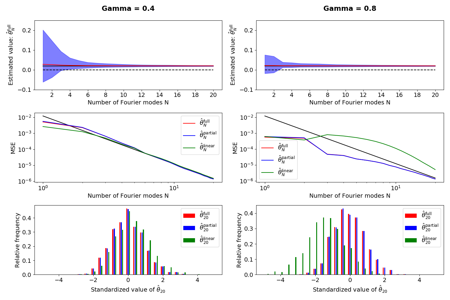
on [0,1][0,1] with Dirichlet boundary conditions and initial condition X0​(x)=sin⁡(π​x)X_{0}(x)=\sin(\pi x). We discretize the equation in Fourier space and simulate N0=100N_{0}=100 modes with a linear-implicit Euler scheme with temporal stepsize htemp=2.5×10⁻⁵h_{\mathrm{temp}}=2.5\times 10^{-5} up to time T=1T=1. The spatial grid is uniform with mesh hspace=5×10⁻⁴h_{\mathrm{space}}=5\times 10^{-4}. The true parameter is θ=0.02\theta=0.02. We have run M=1000M=1000 Monte-Carlo simulations for each of the choices γ=0.4\gamma=0.4 and γ=0.8\gamma=0.8. In any case, we have set α=γ\alpha=\gamma. Remember that in this setting all estimators are asymptotically normal.

Refer to caption
Figure 1. The left column corresponds to the case γ=0.4\gamma=0.4, the right column to the case γ=0.8\gamma=0.8. First row: The median (red) and the 2.52.5-percentile as well as the 97.597.5-percentile (boundaries of the blue region) of M=1000M=1000 Monte-Carlo simulations of θ^Nfull\hat{\theta}^{\mathrm{full}}_{N} are plotted. The solid black line represents the true parameter θ=0.02\theta=0.02, the dashed line is plotted at zero. Second row: The mean squared error (MSE), given by the term 1M​∑i=1M(θ^N,i−θ)2\frac{1}{M}\sum_{i=1}^{M}(\hat{\theta}_{N,i}-\theta)^{2}, is plotted against the squared rate function N↦(V​N−32)2N\mapsto(\sqrt{V}N^{-\frac{3}{2}})^{2}, where VV is the asymptotic variance from Theorem 1.2 and θ^N\hat{\theta}_{N} any of the three estimators. Third row: Histogram of the standardized values of θ^20\hat{\theta}_{20}, i.e. the values of N32V​(θ^N−θ)\frac{N^{\frac{3}{2}}}{\sqrt{V}}(\hat{\theta}_{N}-\theta) for N=20N=20. Each bin has a width of 0.40.4. Outliers outside the range [−5,5][-5,5] are put into the leftmost (or rightmost, resp.) bin.

Figure 1 illustrates consistency, the convergence rate and the asymptotic distribution from Theorem 1.2. As expected, the values of θ^Nfull\hat{\theta}^{\mathrm{full}}_{N} and θ^Npartial\hat{\theta}^{\mathrm{partial}}_{N} are closer to each other than to θ^Nlinear\hat{\theta}^{\mathrm{linear}}_{N}. Note that the quality of θ^Nlinear\hat{\theta}^{\mathrm{linear}}_{N} in this simulation depends on the level of noise given by γ\gamma, with decreasing accuracy under smooth noise. Our interpretation is that the nonlinearity becomes more highlighted if the noise is less rough.

We mention that for simulations with even larger values of γ\gamma (take γ=1.3\gamma=1.3), the values of θ^Nlinear\hat{\theta}^{\mathrm{linear}}_{N} are mostly negative and therefore not related to the true parameter, while θ^Nfull\hat{\theta}^{\mathrm{full}}_{N} and θ^Npartial\hat{\theta}^{\mathrm{partial}}_{N} stay consistent. Of course, this effect may be influenced by the number of Fourier modes N0N_{0} used for the simulation.

4. Proof of Theorem 1.2

We follow closely the arguments which have been given in [9] for the special case of the Navier–Stokes equations in two dimensions. Using a slightly different version of the central limit theorem (CLT) for local martingales, we obtain a direct proof of the asymptotic normality for θ^Nfull\hat{\theta}^{\mathrm{full}}_{N}.

4.1. Properties of the Linear Process

First, we recall briefly some results for the case F=0F=0. Consider the linear equation

(35) d​X¯t=θ​A​X¯t​d​t+B​d​Wt,X¯0=0,\mathrm{d}\overline{X}_{t}=\theta A\overline{X}_{t}\mathrm{d}t+B\mathrm{d}W_{t},\quad\overline{X}_{0}=0,

where B=(−A)−γB=(-A)^{-\gamma}. We define x¯k:=(X¯,Φk)H\overline{x}^{k}:=(\overline{X},\Phi_{k})_{H}. Then the x¯k\overline{x}^{k} are independent one-dimensional Ornstein–Uhlenbeck processes

(36) d​x¯tk=−θ​λk​x¯tk​d​t+λk−γ​d​Wtk,x¯0k=0,\mathrm{d}\overline{x}^{k}_{t}=-\theta\lambda_{k}\overline{x}^{k}_{t}\mathrm{d}t+\lambda_{k}^{-\gamma}\mathrm{d}W^{k}_{t},\quad\overline{x}^{k}_{0}=0,

where (Wk)k∈ℕ(W^{k})_{k\in\mathbb{N}} are independent one-dimensional Brownian motions, and the solutions have the explicit representation

(37) x¯tk=λk−γ​∫0te−θ​λk​(t−s)​d​Wsk.\overline{x}^{k}_{t}=\lambda_{k}^{-\gamma}\int_{0}^{t}e^{-\theta\lambda_{k}(t-s)}\mathrm{d}W^{k}_{s}.
Lemma 4.1 (cf. [9, 27]).

It holds that

  1. (i)

    𝔼​∫0T(x¯tk)2​𝑑t≍T​Λ−(2​γ+1)2​θ​k−β⁡(2​γ+1)\mathbb{E}\int_{0}^{T}(\overline{x}^{k}_{t})^{2}\mathrm{d}t\asymp\frac{T\Lambda^{-(2\gamma+1)}}{2\theta}k^{-\beta(2\gamma+1)} and

  2. (ii)

    Var​∫0T(x¯tk)2​𝑑t≍T​Λ−(4​γ+3)2​θ3​k−β⁡(4​γ+3)\mathrm{Var}\int_{0}^{T}(\overline{x}^{k}_{t})^{2}\mathrm{d}t\asymp\frac{T\Lambda^{-(4\gamma+3)}}{2\theta^{3}}k^{-\beta(4\gamma+3)}

as k→∞k\rightarrow\infty.

Sketch of proof.

Use that x¯sk\overline{x}^{k}_{s} and x¯tk\overline{x}^{k}_{t}, s≤ts\leq t, are jointly Gaussian with mean zero and

𝔼⁡[x¯sk​x¯tk]=λk−(2​γ+1)2​θ​(e−θ​λk​(t−s)−e−θ​λk​(t+s)).\mathbb{E}[\overline{x}^{k}_{s}\overline{x}^{k}_{t}]=\frac{\lambda_{k}^{-(2\gamma+1)}}{2\theta}(e^{-\theta\lambda_{k}(t-s)}-e^{-\theta\lambda_{k}(t+s)}).

Now (i)(i) follows with the help of 𝔼​∫0T(x¯tk)2​𝑑t=∫0T𝔼​(x¯tk)2​𝑑t\mathbb{E}\int_{0}^{T}(\overline{x}^{k}_{t})^{2}\mathrm{d}t=\int_{0}^{T}\mathbb{E}(\overline{x}^{k}_{t})^{2}\mathrm{d}t. For (i​i)(ii), use

𝔼⁡[(x¯sk)2​(x¯tk)2]=Var⁡[x¯sk]​Var​[x¯tk]+2​Cov​(x¯sk,x¯tk)2\mathbb{E}[(\overline{x}^{k}_{s})^{2}(\overline{x}^{k}_{t})^{2}]=\mathrm{Var}[\overline{x}^{k}_{s}]\mathrm{Var}[\overline{x}^{k}_{t}]+2\mathrm{Cov}(\overline{x}^{k}_{s},\overline{x}^{k}_{t})^{2}

and 𝔼​(∫0T(x¯tk)2​𝑑t)2=2​∫0T∫0t𝔼⁡[(x¯sk)2​(x¯tk)2]​𝑑s​𝑑t\mathbb{E}\left(\int_{0}^{T}(\overline{x}^{k}_{t})^{2}\mathrm{d}t\right)^{2}=2\int_{0}^{T}\int_{0}^{t}\mathbb{E}[(\overline{x}^{k}_{s})^{2}(\overline{x}^{k}_{t})^{2}]\mathrm{d}s\mathrm{d}t. ∎

We write X¯N:=PN​X¯\overline{X}^{N}:=P_{N}\overline{X}. By multiplying the asymptotic representations from Lemma 4.1 with Λ2​α+2​kβ⁡(2​α+2)\Lambda^{2\alpha+2}k^{\beta(2\alpha+2)} and Λ4​α+4​kβ⁡(4​α+4)\Lambda^{4\alpha+4}k^{\beta(4\alpha+4)}, respectively, and summing up to index NN, we obtain the following cumulative version if α>γ−1+β−12\alpha>\gamma-\frac{1+\beta^{-1}}{2}:

(38) 𝔼​∫0T|(−A)1+α​X¯tN|H2​𝑑t≍Cα𝔼​Nβ⁡(2​α−2​γ+1)+1,\mathbb{E}\int_{0}^{T}|(-A)^{1+\alpha}\overline{X}^{N}_{t}|_{H}^{2}\mathrm{d}t\asymp C^{\mathbb{E}}_{\alpha}N^{\beta(2\alpha-2\gamma+1)+1},

and if α>γ−1+β−14\alpha>\gamma-\frac{1+\beta^{-1}}{4}:

(39) Var​∫0T|(−A)1+α​X¯tN|H2​𝑑t≍CαVar​Nβ⁡(4​α−4​γ+1)+1,\mathrm{Var}\int_{0}^{T}|(-A)^{1+\alpha}\overline{X}^{N}_{t}|_{H}^{2}\mathrm{d}t\asymp C^{\mathrm{Var}}_{\alpha}N^{\beta(4\alpha-4\gamma+1)+1},

where

Cα𝔼=C𝔼​(θ,T,Λ,β,γ,α)=T​Λ2​α−2​γ+12​θ​(β⁡(2​α−2​γ+1)+1),CαVar=CVar​(θ,T,Λ,β,γ,α)=T​Λ4​α−4​γ+12​θ3​(β⁡(4​α−4​γ+1)+1).\begin{matrix}C^{\mathbb{E}}_{\alpha}&=&C^{\mathbb{E}}(\theta,T,\Lambda,\beta,\gamma,\alpha)&=&\frac{T\Lambda^{2\alpha-2\gamma+1}}{2\theta(\beta(2\alpha-2\gamma+1)+1)},\\ C^{\mathrm{Var}}_{\alpha}&=&C^{\mathrm{Var}}(\theta,T,\Lambda,\beta,\gamma,\alpha)&=&\frac{T\Lambda^{4\alpha-4\gamma+1}}{2\theta^{3}(\beta(4\alpha-4\gamma+1)+1)}.\end{matrix}
Lemma 4.2.

Let α>γ−1+β−14\alpha>\gamma-\frac{1+\beta^{-1}}{4}. Then

(40) ∫0T|(−A)1+α​X¯tN|H2​𝑑t𝔼​∫0T|(−A)1+α​X¯tN|H2​𝑑t→1\frac{\int_{0}^{T}|(-A)^{1+\alpha}\overline{X}^{N}_{t}|_{H}^{2}\mathrm{d}t}{\mathbb{E}\int_{0}^{T}|(-A)^{1+\alpha}\overline{X}^{N}_{t}|_{H}^{2}\mathrm{d}t}\rightarrow 1

as N→∞N\rightarrow\infty in probability.77 7 Using the strong law of large numbers [34], one can easily show that the convergence holds even almost surely, see [9].

Proof.

Taking into account asymptotic equivalence, we obtain

ℙ⁡(|∫0T|(−A)1+α​X¯tN|H2​𝑑t𝔼​∫0T|(−A)1+α​X¯tN|H2​𝑑t−1|>ϵ)\displaystyle\mathbb{P}\left(\left|\frac{\int_{0}^{T}|(-A)^{1+\alpha}\overline{X}^{N}_{t}|_{H}^{2}\mathrm{d}t}{\mathbb{E}\int_{0}^{T}|(-A)^{1+\alpha}\overline{X}^{N}_{t}|_{H}^{2}\mathrm{d}t}-1\right|>\epsilon\right) ≤Var​∫0T|(−A)1+α​X¯tN|H2​𝑑tϵ2​(𝔼​∫0T|(−A)1+α​X¯tN|H2​𝑑t)2\displaystyle\leq\frac{\mathrm{Var}\int_{0}^{T}|(-A)^{1+\alpha}\overline{X}^{N}_{t}|_{H}^{2}\mathrm{d}t}{\epsilon^{2}\left(\mathbb{E}\int_{0}^{T}|(-A)^{1+\alpha}\overline{X}^{N}_{t}|_{H}^{2}\mathrm{d}t\right)^{2}}
≲Nβ⁡(4​α−4​γ+1)+1Nβ⁡(4​α−4​γ+2)+2=N−(β+1),\displaystyle\lesssim\frac{N^{\beta(4\alpha-4\gamma+1)+1}}{N^{\beta(4\alpha-4\gamma+2)+2}}=N^{-(\beta+1)},

which goes to zero as N→∞N\rightarrow\infty. ∎

We close this section by giving the precise regularity for the linear process X¯\overline{X}.

Proposition 4.3.

The unique solution X¯\overline{X} to (35) satisfies X¯∈C⁡([0,T],D⁡((−A)ρ+12))\overline{X}\in C([0,T];D((-A)^{\rho+\frac{1}{2}})) a.s. for ρ<ρ∗\rho<\rho^{*}, where

(41) ρ∗=γ−β−12.\rho^{*}=\gamma-\frac{\beta^{-1}}{2}.

In particular, X¯∈R⁡(ρ)\overline{X}\in R(\rho) for these ρ\rho. Conversely, X¯∉R⁡(ρ∗)\overline{X}\notin R(\rho^{*}) a.s.

Proof.

Let ρ<ρ∗\rho<\rho^{*}. It suffices to prove that Y¯:=(−A)ρ+12​X¯∈C⁡([0,T],H)\overline{Y}:=(-A)^{\rho+\frac{1}{2}}\overline{X}\in C([0,T];H). Given that Y¯\overline{Y} satisfies

(42) d​Y¯t=θ​A​Y¯t​d​t+(−A)ρ+12−γ​d​Wt,Y¯0=0,\mathrm{d}\overline{Y}_{t}=\theta A\overline{Y}_{t}\mathrm{d}t+(-A)^{\rho+\frac{1}{2}-\gamma}\mathrm{d}W_{t},\quad\overline{Y}_{0}=0,

this follows from the factorization formula [12, Section 5.3] once we know that

(43) ∫01t−2​δ​|S⁡(t)​(−A)ρ+12−γ|H​S2​𝑑t<∞\int_{0}^{1}t^{-2\delta}|S(t)(-A)^{\rho+\frac{1}{2}-\gamma}|_{HS}^{2}\mathrm{d}t<\infty

for some δ∈(0,12)\delta\in(0,\frac{1}{2}), where SS is the strongly continuous semigroup generated by AA and |⋅|H​S|\cdot|_{HS} denotes the Hilbert-Schmidt norm.88 8 More precisely: (43) with δ=0\delta=0 yields the existence of a unique solution in HH to (42), and if δ\delta can be chosen in (0,12)(0,\frac{1}{2}), this solution is continuous in time. Indeed:

∫01t−2​δ​|S⁡(t)​(−A)ρ+12−γ|H​S2​𝑑t\displaystyle\int_{0}^{1}t^{-2\delta}|S(t)(-A)^{\rho+\frac{1}{2}-\gamma}|_{HS}^{2}\mathrm{d}t =∑k=1∞∫01t−2​δ​e−2​θ​λk​t​λk2​ρ+1−2​γ​𝑑t\displaystyle=\sum_{k=1}^{\infty}\int_{0}^{1}t^{-2\delta}e^{-2\theta\lambda_{k}t}\lambda_{k}^{2\rho+1-2\gamma}\mathrm{d}t
≤∑k=1∞λk2​ρ+1−2​γ​∫0∞(s2​θ​λk)−2​δ​e−s​12​θ​λk​𝑑s\displaystyle\leq\sum_{k=1}^{\infty}\lambda_{k}^{2\rho+1-2\gamma}\int_{0}^{\infty}\left(\frac{s}{2\theta\lambda_{k}}\right)^{-2\delta}e^{-s}\frac{1}{2\theta\lambda_{k}}\mathrm{d}s
=∑k=1∞λk2​ρ−2​γ+2​δ​(2​θ)2​δ−1​Γ​(1−2​δ)≲∑k=1∞kβ⁡(2​ρ−2​γ+2​δ).\displaystyle=\sum_{k=1}^{\infty}\lambda_{k}^{2\rho-2\gamma+2\delta}(2\theta)^{2\delta-1}\Gamma(1-2\delta)\lesssim\sum_{k=1}^{\infty}k^{\beta(2\rho-2\gamma+2\delta)}.

Here, Γ\Gamma is the Gamma function. The last sum is finite if β⁡(2​ρ−2​γ+2​δ)<−1\beta(2\rho-2\gamma+2\delta)<-1, i.e. ρ<ρ∗−δ\rho<\rho^{*}-\delta. Now δ∈(0,12)\delta\in(0,\frac{1}{2}) can be chosen sufficiently small. Conversely, the discussion leading to (38) shows that

(44) 𝔼​∫0T|(−A)ρ∗+12​X¯tN|H2​𝑑t→∞\mathbb{E}\int_{0}^{T}|(-A)^{\rho^{*}+\frac{1}{2}}\overline{X}^{N}_{t}|_{H}^{2}\mathrm{d}t\rightarrow\infty

as N→∞N\rightarrow\infty, and by Lemma 4.2, we have even a.s. pathwise divergence (take an a.s. converging subsequence in the statement of the Lemma). Hence X¯∉L2​([0,T],D⁡((−A)ρ∗+12))\overline{X}\notin L^{2}([0,T];D((-A)^{\rho^{*}+\frac{1}{2}})) almost surely, and the claim follows. ∎

4.2. Asymptotic Behaviour in the Semilinear Case

4.2.1. Proof of Proposition 1.1 (ii)

Assuming that (Aρ)(A_{\rho}) and (Sρ′)(S^{\prime}_{\rho}) hold for some ρ∈[0,ρ∗)\rho\in[0,\rho^{*}), we define X~:=X−X¯\widetilde{X}:=X-\overline{X} and X~N:=PN​X~\widetilde{X}^{N}:=P_{N}\widetilde{X}, where as before X¯\overline{X} is the solution to (35). These processes are well-defined and satisfy

(45) X~tN=X0N+∫0t(θ​A​X~sN+F⁡(s,X¯s+X~s))​𝑑s.\widetilde{X}^{N}_{t}=X^{N}_{0}+\int_{0}^{t}(\theta A\widetilde{X}^{N}_{s}+F(s,\overline{X}_{s}+\widetilde{X}_{s}))\mathrm{d}s.

Calculations similar to those in Lemma A.3 show99 9 Note, however, that the Galerkin approximants to X~\widetilde{X} we use in this section are not identical to the approximants from Lemma A.3, which satisfy (78) rather than (45)

(46) sup0≤t≤T|X~tN|ρ+ϵρ2+θ​∫0T|X~tN|ρ+12+ϵρ2​𝑑t≤|X0N|ρ+ϵρ2+Cθ​∫0T|PN​F​(t,X¯t+X~t)|ρ−12+ϵρ2​𝑑t.\sup_{0\leq t\leq T}|\widetilde{X}^{N}_{t}|_{\rho+\epsilon_{\rho}}^{2}+\theta\int_{0}^{T}|\widetilde{X}^{N}_{t}|_{\rho+\frac{1}{2}+\epsilon_{\rho}}^{2}\mathrm{d}t\leq|X^{N}_{0}|_{\rho+\epsilon_{\rho}}^{2}+C_{\theta}\int_{0}^{T}|P_{N}F(t,\overline{X}_{t}+\widetilde{X}_{t})|_{\rho-\frac{1}{2}+\epsilon_{\rho}}^{2}\mathrm{d}t.

The nonlinear term is estimated as follows:

∫0T|PN​F​(t,X¯t+X~t)|ρ−12+ϵρ2​𝑑t\displaystyle\int_{0}^{T}|P_{N}F(t,\overline{X}_{t}+\widetilde{X}_{t})|_{\rho-\frac{1}{2}+\epsilon_{\rho}}^{2}\mathrm{d}t ≤∫0T(fρ​(T)+|X¯t+X~t|ρ+122)​gρ​(|X¯t+X~t|ρ)​𝑑t\displaystyle\leq\int_{0}^{T}(f_{\rho}(T)+|\overline{X}_{t}+\widetilde{X}_{t}|_{\rho+\frac{1}{2}}^{2})g_{\rho}(|\overline{X}_{t}+\widetilde{X}_{t}|_{\rho})\mathrm{d}t
≤sup0≤t≤Tgρ​(|X¯t+X~t|ρ)​∫0T(fρ​(t)+|X¯t+X~t|ρ+122)​𝑑t<∞,\displaystyle\leq\sup_{0\leq t\leq T}g_{\rho}(|\overline{X}_{t}+\widetilde{X}_{t}|_{\rho})\int_{0}^{T}\left(f_{\rho}(t)+|\overline{X}_{t}+\widetilde{X}_{t}|_{\rho+\frac{1}{2}}^{2}\right)\mathrm{d}t<\infty,

so (X~N)N∈ℕ(\widetilde{X}^{N})_{N\in\mathbb{N}} is bounded in R⁡(ρ+ϵρ)R(\rho+\epsilon_{\rho}), thus X~∈R⁡(ρ+ϵρ)\widetilde{X}\in R(\rho+\epsilon_{\rho}). We have proven:

Lemma 4.4.

If (Aρ)(A_{\rho}) and (Sρ′)(S^{\prime}_{\rho}) hold for some ρ∈[0,ρ∗)\rho\in[0,\rho^{*}), then X~∈R⁡(ρ+ϵρ)\widetilde{X}\in R(\rho+\epsilon_{\rho}) a.s.

We finish the proof of Proposition 1.1 (ii) with the following Lemma:

Lemma 4.5.

If (Aρ)(A_{\rho}) and (Sρ′)(S^{\prime}_{\rho}) hold for some ρ∈[0,ρ∗)\rho\in[0,\rho^{*}) with ρ+ϵρ>ρ∗\rho+\epsilon_{\rho}>\rho^{*}, then almost surely X∈R⁡(ρ∗−δ)X\in R(\rho^{*}-\delta) for δ>0\delta>0 and X∉R⁡(ρ∗)X\notin R(\rho^{*}).

Proof.

This follows from X¯∈R⁡(ρ∗−δ)\overline{X}\in R(\rho^{*}-\delta) for δ>0\delta>0, X¯∉R⁡(ρ∗)\overline{X}\notin R(\rho^{*}) and X~∈R⁡(ρ∗)\widetilde{X}\in R(\rho^{*}) almost surely. ∎

4.2.2. An Asymptotic Growth Property

Proposition 4.6.

Assume that (Rη)(R_{\eta}) holds for some η>0\eta>0. Let α>γ−1+β−14\alpha>\gamma-\frac{1+\beta^{-1}}{4}. Then

(47) ∫0T|(−A)1+α​XtN|H2​𝑑t𝔼​∫0T|(−A)1+α​X¯tN|H2​𝑑t→1\frac{\int_{0}^{T}|(-A)^{1+\alpha}X^{N}_{t}|_{H}^{2}\mathrm{d}t}{\mathbb{E}\int_{0}^{T}|(-A)^{1+\alpha}\overline{X}^{N}_{t}|_{H}^{2}\mathrm{d}t}\rightarrow 1

as N→∞N\rightarrow\infty in probability.1010 10 As in Lemma 4.2, almost sure convergence holds in fact.

Proof.

We set

(48) Z1,N:=(−A)1+α​X¯N(𝔼​∫0T|(−A)1+α​X¯tN|H2​𝑑t)12,Z2,N:=(−A)1+α​X~N(𝔼​∫0T|(−A)1+α​X¯tN|H2​𝑑t)12,Z^{1,N}:=\frac{(-A)^{1+\alpha}\overline{X}^{N}}{\left(\mathbb{E}\int_{0}^{T}|(-A)^{1+\alpha}\overline{X}^{N}_{t}|_{H}^{2}\mathrm{d}t\right)^{\frac{1}{2}}},\quad Z^{2,N}:=\frac{(-A)^{1+\alpha}\widetilde{X}^{N}}{\left(\mathbb{E}\int_{0}^{T}|(-A)^{1+\alpha}\overline{X}^{N}_{t}|_{H}^{2}\mathrm{d}t\right)^{\frac{1}{2}}},

and by Lemma 4.2,

(49) ℙ⁡(∫0T|Zt1,N|H2​𝑑t>2)≤ℙ⁡(|∫0T|Zt1,N|H2​𝑑t−1|>1)→0,\mathbb{P}\left(\int_{0}^{T}|Z^{1,N}_{t}|_{H}^{2}\mathrm{d}t>2\right)\leq\mathbb{P}\left(\left|\int_{0}^{T}|Z^{1,N}_{t}|_{H}^{2}\mathrm{d}t-1\right|>1\right)\rightarrow 0,

i.e. Z1,NZ^{1,N} is bounded in probability. Now choose α′∈(ρ∗−12,ρ∗−12+η)\alpha^{\prime}\in(\rho^{*}-\frac{1}{2},\rho^{*}-\frac{1}{2}+\eta) with α′<α\alpha^{\prime}<\alpha. Then

∫0T|Zt2,N|H2​𝑑t\displaystyle\int_{0}^{T}|Z^{2,N}_{t}|_{H}^{2}\mathrm{d}t =∫0T|(−A)1+α​X~tN|H2​𝑑t𝔼​∫0T|(−A)1+α​X¯tN|H2​𝑑t≲N2​β​(α−α′)​∫0T|(−A)1+α′​X~tN|H2​𝑑t𝔼​∫0T|(−A)1+α​X¯tN|H2​𝑑t\displaystyle=\frac{\int_{0}^{T}|(-A)^{1+\alpha}\widetilde{X}^{N}_{t}|_{H}^{2}\mathrm{d}t}{\mathbb{E}\int_{0}^{T}|(-A)^{1+\alpha}\overline{X}^{N}_{t}|_{H}^{2}\mathrm{d}t}\lesssim\frac{N^{2\beta(\alpha-\alpha^{\prime})}\int_{0}^{T}|(-A)^{1+\alpha^{\prime}}\widetilde{X}^{N}_{t}|_{H}^{2}\mathrm{d}t}{\mathbb{E}\int_{0}^{T}|(-A)^{1+\alpha}\overline{X}^{N}_{t}|_{H}^{2}\mathrm{d}t}
≲N2​β​(α−α′)Nβ⁡(2​α−2​ρ∗+1)​∫0T|(−A)1+α′​X~tN|H2​𝑑t=N−β⁡(2​α′−2​ρ∗+1)​∫0T|(−A)1+α′​X~tN|H2​𝑑t,\displaystyle\hskip-56.9055pt\lesssim\frac{N^{2\beta(\alpha-\alpha^{\prime})}}{N^{\beta(2\alpha-2\rho^{*}+1)}}\int_{0}^{T}|(-A)^{1+\alpha^{\prime}}\widetilde{X}^{N}_{t}|_{H}^{2}\mathrm{d}t=N^{-\beta(2\alpha^{\prime}-2\rho^{*}+1)}\int_{0}^{T}|(-A)^{1+\alpha^{\prime}}\widetilde{X}^{N}_{t}|_{H}^{2}\mathrm{d}t,

where we used (4) and (38). The last term converges to zero a.s. because ∫0T|(−A)1+α′​X~tN|H2​𝑑t<∞\int_{0}^{T}|(-A)^{1+\alpha^{\prime}}\widetilde{X}^{N}_{t}|_{H}^{2}\mathrm{d}t<\infty almost surely due to condition (Rη)(R_{\eta}). Finally,

ℙ⁡(|∫0T(Zt1,N,Zt2,N)H​𝑑t|2>ϵ)\displaystyle\mathbb{P}\left(\left|\int_{0}^{T}(Z^{1,N}_{t},Z^{2,N}_{t})_{H}\mathrm{d}t\right|^{2}>\epsilon\right) ≤ℙ⁡(∫0T|Zt1,N|H2​𝑑t​∫0T|Zt2,N|H2​𝑑t>ϵ)\displaystyle\leq\mathbb{P}\left(\int_{0}^{T}|Z^{1,N}_{t}|_{H}^{2}\mathrm{d}t\int_{0}^{T}|Z^{2,N}_{t}|_{H}^{2}\mathrm{d}t>\epsilon\right)
≤ℙ⁡(∫0T|Zt1,N|H2​𝑑t≥2)+ℙ⁡(∫0T|Zt2,N|H2​𝑑t≥ϵ2),\displaystyle\leq\mathbb{P}\left(\int_{0}^{T}|Z^{1,N}_{t}|_{H}^{2}\mathrm{d}t\geq 2\right)+\mathbb{P}\left(\int_{0}^{T}|Z^{2,N}_{t}|_{H}^{2}\mathrm{d}t\geq\frac{\epsilon}{2}\right),

which converges to zero as N→∞N\rightarrow\infty. The claim follows easily. ∎

4.3. Analysis of the Estimators

Throughout this section we work under the assumptions of Theorem 1.2. Inserting (8) into (11), (13) and (14), the estimators can be written in the form

(50) θ^Nfull−θ=−∫0T⟨(−A)1+2​α​XtN,PN​B​d​Wt⟩∫0T|(−A)1+α​XtN|H2​𝑑t,\hat{\theta}^{\mathrm{full}}_{N}-\theta=-\frac{\int_{0}^{T}\langle(-A)^{1+2\alpha}X^{N}_{t},P_{N}B\mathrm{d}W_{t}\rangle}{\int_{0}^{T}|(-A)^{1+\alpha}X^{N}_{t}|_{H}^{2}\mathrm{d}t},
(51) θ^Npartial−θ=−∫0T⟨(−A)1+2​α​XtN,PN​B​d​Wt⟩∫0T|(−A)1+α​XtN|H2​𝑑t−biasN​(X)+biasN​(XN),\hat{\theta}^{\mathrm{partial}}_{N}-\theta=-\frac{\int_{0}^{T}\langle(-A)^{1+2\alpha}X^{N}_{t},P_{N}B\mathrm{d}W_{t}\rangle}{\int_{0}^{T}|(-A)^{1+\alpha}X^{N}_{t}|_{H}^{2}\mathrm{d}t}-\mathrm{bias}_{N}(X)+\mathrm{bias}_{N}(X^{N}),
(52) θ^Nlinear−θ=−∫0T⟨(−A)1+2​α​XtN,PN​B​d​Wt⟩∫0T|(−A)1+α​XtN|H2​𝑑t−biasN​(X).\hat{\theta}^{\mathrm{linear}}_{N}-\theta=-\frac{\int_{0}^{T}\langle(-A)^{1+2\alpha}X^{N}_{t},P_{N}B\mathrm{d}W_{t}\rangle}{\int_{0}^{T}|(-A)^{1+\alpha}X^{N}_{t}|_{H}^{2}\mathrm{d}t}-\mathrm{bias}_{N}(X).

We prove asymptotic normality of θ^Nfull\hat{\theta}^{\mathrm{full}}_{N} by means of the following CLT, which is a special case of [24, Theorem 5.5.4 (I)] and [19, Theorem VIII.4.17]:

Lemma 4.7.

Let (MN)N∈ℕ(M^{N})_{N\in\mathbb{N}} be a sequence of continuous local martingales with M0N=0M^{N}_{0}=0, let T>0T>0 and V>0V>0. Assume

(53) ⟨MN⟩T→ℙV\langle M^{N}\rangle_{T}\xrightarrow{\mathbb{P}}V

as N→∞N\rightarrow\infty. Then

(54) MTN→𝑑𝒩⁡(0,V).M^{N}_{T}\xrightarrow{d}\mathcal{N}(0,V).

In the present situation, we set

(55) MtN:=N−β⁡(2​α−2​γ)−β+12​∫0t⟨(−A)1+2​α​XtN,PN​B​d​Wt⟩M^{N}_{t}:=N^{-\beta(2\alpha-2\gamma)-\frac{\beta+1}{2}}\int_{0}^{t}\langle(-A)^{1+2\alpha}X^{N}_{t},P_{N}B\mathrm{d}W_{t}\rangle

for α>γ−1+β−18\alpha>\gamma-\frac{1+\beta^{-1}}{8} and note that these are continuous local martingales with

(56) ⟨MN⟩t=N−β⁡(4​α−4​γ+1)−1​∫0t|(−A)1+2​α−γ​XsN|H2​𝑑s<∞\langle M^{N}\rangle_{t}=N^{-\beta(4\alpha-4\gamma+1)-1}\int_{0}^{t}|(-A)^{1+2\alpha-\gamma}X^{N}_{s}|_{H}^{2}\mathrm{d}s<\infty

almost surely. Proposition 4.6 and (38) give ⟨MN⟩T→C2​α−γ𝔼\langle M^{N}\rangle_{T}\rightarrow C^{\mathbb{E}}_{2\alpha-\gamma} in probability. The CLT gives MTN→𝑑𝒩⁡(0,C2​α−γ𝔼)M^{N}_{T}\xrightarrow{d}\mathcal{N}(0,C^{\mathbb{E}}_{2\alpha-\gamma}). Another application of Proposition 4.6 together with Slutsky’s lemma yields

(57) Nβ+12​∫0T⟨(−A)1+2​α​XtN,PN​B​d​Wt⟩∫0T|(−A)1+α​XtN|H2​𝑑t→𝑑𝒩⁡(0,C2​α−γ𝔼(Cα𝔼)2).N^{\frac{\beta+1}{2}}\frac{\int_{0}^{T}\langle(-A)^{1+2\alpha}X^{N}_{t},P_{N}B\mathrm{d}W_{t}\rangle}{\int_{0}^{T}|(-A)^{1+\alpha}X^{N}_{t}|_{H}^{2}\mathrm{d}t}\xrightarrow{d}\mathcal{N}\left(0,\frac{C^{\mathbb{E}}_{2\alpha-\gamma}}{(C^{\mathbb{E}}_{\alpha})^{2}}\right).

Rearranging the terms, we have proven part (ii) from Theorem 1.2.

Remark.

It is not necessary to perform a perturbation argument to prove asymptotic normality for θ^Nfull\hat{\theta}^{\mathrm{full}}_{N}, i.e. we do not have to bound a remainder integral of the type ∫0T⟨(−A)1+2​α​X~tN,PN​B​d​Wt⟩\int_{0}^{T}\langle(-A)^{1+2\alpha}\widetilde{X}^{N}_{t},P_{N}B\mathrm{d}W_{t}\rangle directly (even if this is not difficult using the Burkholder–Davis–Gundy inequality).

Next, we prove consistency for the remaining estimators. Taking into account (51) and (52), part (i) and (iv) from Theorem 1.2 follow immediately from the following lemma:

Lemma 4.8.

Let ρ∈[0,ρ∗)\rho\in[0,\rho^{*}). Assume (Aρ)(A_{\rho}) and either (Sρ)(S_{\rho}) or (Sρ′)(S^{\prime}_{\rho}) hold with ρ+ϵρ>ρ∗\rho+\epsilon_{\rho}>\rho^{*}, assume further X~∈R⁡(ρ+ϵρ)\widetilde{X}\in R(\rho+\epsilon_{\rho}). Let α>γ−1+β−18\alpha>\gamma-\frac{1+\beta^{-1}}{8}.

  1. (i)

    If ρ+ϵρ−ρ∗>1+β−12\rho+\epsilon_{\rho}-\rho^{*}>\frac{1+\beta^{-1}}{2}, then a.s.

    (58) limN→∞Nβ+12​biasN​(X)=0.\lim_{N\rightarrow\infty}N^{\frac{\beta+1}{2}}\mathrm{bias}_{N}(X)=0.
  2. (ii)

    Otherwise,

    (59) limN→∞Nβ​ϵ​biasN​(X)=0\lim_{N\rightarrow\infty}N^{\beta\epsilon}\mathrm{bias}_{N}(X)=0

    a.s. for any ϵ<ρ+ϵρ−ρ∗\epsilon<\rho+\epsilon_{\rho}-\rho^{*}.

The same is true for biasN​(XN)\mathrm{bias}_{N}(X^{N}).

Proof.

We prove the statement just for biasN​(X)\mathrm{bias}_{N}(X), the proof for the remaining case is identical up to trivial norm estimates. If ρ+ϵρ−ρ∗≤1+β−12\rho+\epsilon_{\rho}-\rho^{*}\leq\frac{1+\beta^{-1}}{2}, choose ϵ∈(0,ρ+ϵρ−ρ∗)\epsilon\in(0,\rho+\epsilon_{\rho}-\rho^{*}), otherwise choose ϵ∈(1+β−12,(2​α−2​ρ∗+1)∧(ρ+ϵρ−ρ∗))\epsilon\in\left(\frac{1+\beta^{-1}}{2},(2\alpha-2\rho^{*}+1)\wedge(\rho+\epsilon_{\rho}-\rho^{*})\right). The latter interval is not empty due to α>γ−1+β−18\alpha>\gamma-\frac{1+\beta^{-1}}{8}. In any case it holds that 2​α>2​ρ∗−1+ϵ2\alpha>2\rho^{*}-1+\epsilon. Now, with κ=2\kappa=2 under (Sρ′)(S^{\prime}_{\rho}) and κ=4\kappa=4 under (Sρ)(S_{\rho}), we have

|∫0T⟨(−A)1+2​αXtN,PNF(t,Xt)⟩V∗Vdt|\displaystyle\left|\int_{0}^{T}{}_{V}\langle(-A)^{1+2\alpha}X^{N}_{t},P_{N}F(t,X_{t})\rangle_{V^{*}}\mathrm{d}t\right|
≤∫0T|(−A)(2​α−2​ρ∗+1−ϵ)+(ρ∗+12−(ρ+ϵρ−ρ∗−ϵ))​XtN|H|​(−A)ρ−12+ϵρ​PN​F​(t,Xt)|H​𝑑t\displaystyle\hskip-113.81102pt\leq\int_{0}^{T}|(-A)^{(2\alpha-2\rho^{*}+1-\epsilon)+(\rho^{*}+\frac{1}{2}-(\rho+\epsilon_{\rho}-\rho^{*}-\epsilon))}X^{N}_{t}|_{H}|(-A)^{\rho-\frac{1}{2}+\epsilon_{\rho}}P_{N}F(t,X_{t})|_{H}\mathrm{d}t
≲Nβ⁡(2​α−2​ρ∗+1−ϵ)​∫0T|XtN|ρ∗+12−(ρ+ϵρ−ρ∗−ϵ)|​PN​F​(t,Xt)|ρ−12+ϵρ​𝑑t\displaystyle\hskip-113.81102pt\lesssim N^{\beta(2\alpha-2\rho^{*}+1-\epsilon)}\int_{0}^{T}|X^{N}_{t}|_{\rho^{*}+\frac{1}{2}-(\rho+\epsilon_{\rho}-\rho^{*}-\epsilon)}|P_{N}F(t,X_{t})|_{\rho-\frac{1}{2}+\epsilon_{\rho}}\mathrm{d}t
≲Nβ⁡(2​α−2​ρ∗+1−ϵ)​(∫0T|XtN|ρ∗+12−(ρ+ϵρ−ρ∗−ϵ)2​𝑑t)12​(∫0T|PN​F​(t,Xt)|ρ−12+ϵρ2​𝑑t)12\displaystyle\hskip-113.81102pt\lesssim N^{\beta(2\alpha-2\rho^{*}+1-\epsilon)}\left(\int_{0}^{T}|X^{N}_{t}|_{\rho^{*}+\frac{1}{2}-(\rho+\epsilon_{\rho}-\rho^{*}-\epsilon)}^{2}\mathrm{d}t\right)^{\frac{1}{2}}\left(\int_{0}^{T}|P_{N}F(t,X_{t})|_{\rho-\frac{1}{2}+\epsilon_{\rho}}^{2}\mathrm{d}t\right)^{\frac{1}{2}}
≲Nβ⁡(2​α−2​ρ∗+1−ϵ)​(∫0T(fρ​(t)+|Xt|ρ+12κ)​gρ​(|Xt|ρ)​𝑑t)12,\displaystyle\hskip-113.81102pt\lesssim N^{\beta(2\alpha-2\rho^{*}+1-\epsilon)}\left(\int_{0}^{T}(f_{\rho}(t)+|X_{t}|_{\rho+\frac{1}{2}}^{\kappa})g_{\rho}(|X_{t}|_{\rho})\mathrm{d}t\right)^{\frac{1}{2}},

where we used X¯,X~∈R⁡(ρ∗−(ρ+ϵρ−ρ∗−ϵ))\overline{X},\widetilde{X}\in R(\rho^{*}-(\rho+\epsilon_{\rho}-\rho^{*}-\epsilon)). Under (Sρ′)(S^{\prime}_{\rho}), the last integral is bounded due to X∈R⁡(ρ)X\in R(\rho) and κ=2\kappa=2. Under (Sρ)(S_{\rho}) we have κ=4\kappa=4. In this case, X¯\overline{X} and X~\widetilde{X} are continuous with values in D⁡((−A)ρ+12)D((-A)^{\rho+\frac{1}{2}}) due to Proposition 4.3 and ϵρ≥12\epsilon_{\rho}\geq\frac{1}{2}, thus

∫0T(fρ​(t)+|Xt|ρ+124)​gρ​(|Xt|ρ)​𝑑t≤sup0≤t≤Tgρ​(|Xt|ρ)​(∫0Tfρ​(t)​𝑑t+T​sup0≤t≤T|Xt|ρ+124)<∞.\int_{0}^{T}(f_{\rho}(t)+|X_{t}|_{\rho+\frac{1}{2}}^{4})g_{\rho}(|X_{t}|_{\rho})\mathrm{d}t\leq\sup_{0\leq t\leq T}g_{\rho}(|X_{t}|_{\rho})\left(\int_{0}^{T}f_{\rho}(t)\mathrm{d}t+T\sup_{0\leq t\leq T}|X_{t}|_{\rho+\frac{1}{2}}^{4}\right)<\infty.

In any case,

(60) lim supN→∞N−β⁡(2​α−2​ρ∗+1−ϵ)|∫0T⟨(−A)1+2​αXtN,PNF(t,Xt)⟩V∗Vdt|<∞,\limsup_{N\rightarrow\infty}N^{-\beta(2\alpha-2\rho^{*}+1-\epsilon)}\left|\int_{0}^{T}{}_{V}\langle(-A)^{1+2\alpha}X^{N}_{t},P_{N}F(t,X_{t})\rangle_{V^{*}}\mathrm{d}t\right|<\infty,

and the claim follows. For (59), we note that ϵ∈(0,ρ+ϵρ−ρ∗)\epsilon\in(0,\rho+\epsilon_{\rho}-\rho^{*}) is arbitrary. ∎

Finally, Theorem 1.2 (iii) follows from (51) and the next lemma.

Lemma 4.9.

Assume (Aρ)(A_{\rho}) and (Tρ)(T_{\rho}) for some ρ≥0\rho\geq 0, let α>γ−1+β−18\alpha>\gamma-\frac{1+\beta^{-1}}{8} and ϵ>0\epsilon>0 such that X∈R⁡(ρ∗−ϵ)X\in R(\rho^{*}-\epsilon) almost surely. Then

(61) Nβ​δρ−2​β​ϵ​(biasN​(X)−biasN​(XN))→a.s.0,N^{\beta\delta_{\rho}-2\beta\epsilon}(\mathrm{bias}_{N}(X)-\mathrm{bias}_{N}(X^{N}))\xrightarrow{a.s.}0,

where δρ\delta_{\rho} is as in (Tρ)(T_{\rho}).

Proof.

We proceed similarly as in Lemma 4.8. Since α>ρ∗−12\alpha>\rho^{*}-\frac{1}{2}, it holds

|∫0T⟨(−A)1+2​αXtN,PNF(t,Xt)−PNF(t,XtN)⟩V∗Vdt|\displaystyle\left|\int_{0}^{T}{}_{V}\langle(-A)^{1+2\alpha}X^{N}_{t},P_{N}F(t,X_{t})-P_{N}F(t,X^{N}_{t})\rangle_{V^{*}}\mathrm{d}t\right|
≤∫0T|(−A)32+2​α−ρ​XtN|H|​(−A)ρ−12​(PN​F​(t,Xt)−PN​F​(t,XtN))|H​𝑑t\displaystyle\hskip-227.62204pt\leq\int_{0}^{T}|(-A)^{\frac{3}{2}+2\alpha-\rho}X^{N}_{t}|_{H}|(-A)^{\rho-\frac{1}{2}}(P_{N}F(t,X_{t})-P_{N}F(t,X^{N}_{t}))|_{H}\mathrm{d}t
≲Nβ⁡(2​α−ρ−ρ∗+ϵ+1)​∫0T|XtN|ρ∗+12−ϵ|​PN​F​(t,Xt)−PN​F​(t,XtN)|ρ−12​𝑑t\displaystyle\hskip-227.62204pt\lesssim N^{\beta(2\alpha-\rho-\rho^{*}+\epsilon+1)}\int_{0}^{T}|X^{N}_{t}|_{\rho^{*}+\frac{1}{2}-\epsilon}|P_{N}F(t,X_{t})-P_{N}F(t,X^{N}_{t})|_{\rho-\frac{1}{2}}\mathrm{d}t
≤Nβ⁡(2​α−ρ−ρ∗+ϵ+1)​(∫0T|XtN|ρ∗+12−ϵ2​𝑑t​∫0T|PN​F​(t,Xt)−PN​F​(t,XtN)|ρ−122​𝑑t)12\displaystyle\hskip-227.62204pt\leq N^{\beta(2\alpha-\rho-\rho^{*}+\epsilon+1)}\left(\int_{0}^{T}|X^{N}_{t}|_{\rho^{*}+\frac{1}{2}-\epsilon}^{2}\mathrm{d}t\int_{0}^{T}|P_{N}F(t,X_{t})-P_{N}F(t,X^{N}_{t})|_{\rho-\frac{1}{2}}^{2}\mathrm{d}t\right)^{\frac{1}{2}}
≲Nβ⁡(2​α−ρ−ρ∗+ϵ+1)​(∫0Thρ​(|Xt|ρ,|XtN|ρ)​|Xt−XtN|ρ+12−δρ2​𝑑t)12\displaystyle\hskip-227.62204pt\lesssim N^{\beta(2\alpha-\rho-\rho^{*}+\epsilon+1)}\left(\int_{0}^{T}h_{\rho}(|X_{t}|_{\rho},|X^{N}_{t}|_{\rho})|X_{t}-X^{N}_{t}|_{\rho+\frac{1}{2}-\delta_{\rho}}^{2}\mathrm{d}t\right)^{\frac{1}{2}}
≲Nβ⁡(2​α−ρ−ρ∗+ϵ+1)−β⁡(δρ+ρ∗−ϵ−ρ)​(∫0T|Xt−XtN|ρ∗+12−ϵ2​𝑑t)12,\displaystyle\hskip-227.62204pt\lesssim N^{\beta(2\alpha-\rho-\rho^{*}+\epsilon+1)-\beta(\delta_{\rho}+\rho^{*}-\epsilon-\rho)}\left(\int_{0}^{T}|X_{t}-X^{N}_{t}|_{\rho^{*}+\frac{1}{2}-\epsilon}^{2}\mathrm{d}t\right)^{\frac{1}{2}},

where we used (5) and the fact that hρh_{\rho} is bounded on [0,sup0≤t≤T|Xt|ρ]2[0,\;\sup_{0\leq t\leq T}|X_{t}|_{\rho}]^{2}. Thus

lim supN→∞N−β⁡(2​α−2​ρ∗+1)+(β​δρ−2​β​ϵ)|∫0T⟨(−A)1+2​αXtN,PNF(t,Xt)−PNF(t,XtN)⟩V∗Vdt|\displaystyle\limsup_{N\rightarrow\infty}N^{-\beta(2\alpha-2\rho^{*}+1)+(\beta\delta_{\rho}-2\beta\epsilon)}\left|\int_{0}^{T}{}_{V}\langle(-A)^{1+2\alpha}X^{N}_{t},P_{N}F(t,X_{t})-P_{N}F(t,X^{N}_{t})\rangle_{V^{*}}\mathrm{d}t\right|
≤C​lim supN→∞(∫0T|Xt−XtN|ρ∗+12−ϵ2​𝑑t)12=0\displaystyle\hskip-170.71652pt\leq C\limsup_{N\rightarrow\infty}\left(\int_{0}^{T}|X_{t}-X^{N}_{t}|_{\rho^{*}+\frac{1}{2}-\epsilon}^{2}\mathrm{d}t\right)^{\frac{1}{2}}=0

a.s. for some C>0C>0 by dominated convergence. ∎

5. The Case of Coupled SPDEs

The same techniques as applied above allow for further generalization. More precisely, XX may be coupled with another state variable X⟂X^{\perp} with state space H⟂H^{\perp}. This leads to a system of the form

(62) d​Xt=(θ​A​XtCLOSE+OPENF⁡(t,Xt,Xt⟂))​d​t+B​d​Wt,d​Xt⟂=F⟂​(t,Xt,Xt⟂)​d​t+B⟂​(t,Xt,Xt⟂)​d​Wt\begin{matrix}\mathrm{d}X_{t}&=&(\theta AX_{t}&+&F(t,X_{t},X^{\perp}_{t}))\mathrm{d}t&+&B\mathrm{d}W_{t},\\ \mathrm{d}X^{\perp}_{t}&=&&&F^{\perp}(t,X_{t},X^{\perp}_{t})\mathrm{d}t&+&B^{\perp}(t,X_{t},X^{\perp}_{t})\mathrm{d}W_{t}\end{matrix}

with initial condition X0∈HX_{0}\in H, X0⟂∈H⟂X^{\perp}_{0}\in H^{\perp}.

Let us describe this setting in more detail. Let ℋ\mathscr{H} be a Hilbert space with inner product (⋅,⋅)ℋ(\cdot,\cdot)_{\mathscr{H}} and H⊆ℋH\subseteq\mathscr{H} a closed subspace with orthogonal complement H⟂H^{\perp}, i.e. ℋ=H⊕H⟂\mathscr{H}=H\oplus H^{\perp}. Let AA be some negative definite self-adjoint operator on HH with compact resolvent and domain D⁡(A)⊂HD(A)\subset H, let 𝒜=A⊕0\mathscr{A}=A\oplus 0 be its trivial continuation to D⁡(𝒜)=D⁡(A)⊕H⟂⊂ℋD(\mathscr{A})=D(A)\oplus H^{\perp}\subset\mathscr{H} given by 𝒜⁡(h,h⟂)=(A​h,0)\mathscr{A}(h,h^{\perp})=(Ah,0). We set V=D⁡((−A)12)V=D((-A)^{\frac{1}{2}}) and 𝒱=D⁡((−𝒜)12)=V⊕H⟂\mathscr{V}=D((-\mathscr{A})^{\frac{1}{2}})=V\oplus H^{\perp}. Consider an equation in ℋ\mathscr{H} of the form

(63) d​𝒳t=(θ​𝒜​𝒳t+ℱ⁡(t,𝒳t))​d​t+ℬ⁡(t,𝒳t)​d​Wt\mathrm{d}\mathscr{X}_{t}=(\theta\mathscr{A}\mathscr{X}_{t}+\mathscr{F}(t,\mathscr{X}_{t}))\mathrm{d}t+\mathscr{B}(t,\mathscr{X}_{t})\mathrm{d}W_{t}

with initial condition 𝒳0∈ℋ\mathscr{X}_{0}\in\mathscr{H}. Here, ℱ:[0,T]×𝒱→𝒱∗\mathscr{F}:[0,T]\times\mathscr{V}\rightarrow\mathscr{V}^{*} is a measurable operator, WW is a cylindrical Wiener process on ℋ\mathscr{H}, and ℬ:[0,T]×𝒱×Ω→L2​(ℋ)\mathscr{B}:[0,T]\times\mathscr{V}\times\Omega\rightarrow L_{2}(\mathscr{H}) is measurable with values in the space of Hilbert–Schmidt operators on ℋ\mathscr{H}. By decomposing 𝒳\mathscr{X}, ℱ\mathscr{F} and ℬ\mathscr{B} as 𝒳=(X,X⟂)\mathscr{X}=(X,X^{\perp}), ℱ=(F,F⟂)\mathscr{F}=(F,F^{\perp}) and ℬ=(B,B⟂)\mathscr{B}=(B,B^{\perp}), we obtain (62).

As before, we assume B=(−A)−γB=(-A)^{-\gamma}, whereas B⟂:[0,T]×𝒱×Ω→H⟂B^{\perp}:[0,T]\times\mathscr{V}\times\Omega\rightarrow H^{\perp} may be arbitrary. The eigenvalues (λk)k∈ℕ(\lambda_{k})_{k\in\mathbb{N}} of −A-A are assumed to satisfy (9). The Sobolev norms on the spaces D⁡((−A)ρ)⊂HD((-A)^{\rho})\subset H and D⁡((−𝒜)ρ)⊂ℋD((-\mathscr{A})^{\rho})\subset\mathscr{H} are given by |x|ρ=|(−A)ρ​x|H|x|_{\rho}=|(-A)^{\rho}x|_{H} and ‖x‖ρ=|(−𝒜)ρ​x|ℋ||x||_{\rho}=|(-\mathscr{A})^{\rho}x|_{\mathscr{H}}, respectively. It is easy to verify that D⁡((−𝒜)ρ)=D⁡((−A)ρ)⊕H⟂D((-\mathscr{A})^{\rho})=D((-A)^{\rho})\oplus H^{\perp} for ρ∈ℝ\rho\in\mathbb{R}. We define

(64) ℛ⁡(ρ):=C⁡([0,T],D⁡((−𝒜)ρ))∩L2​([0,T],D⁡((−𝒜)ρ+12))\mathscr{R}(\rho):=C([0,T];D((-\mathscr{A})^{\rho}))\cap L^{2}([0,T];D((-\mathscr{A})^{\rho+\frac{1}{2}}))

and

(65) R⁡(ρ):=C⁡([0,T],D⁡((−A)ρ))∩L2​([0,T],D⁡((−A)ρ+12))R(\rho):=C([0,T];D((-A)^{\rho}))\cap L^{2}([0,T];D((-A)^{\rho+\frac{1}{2}}))

and say that (63) has a weak solution in ℛ⁡(ρ)\mathscr{R}(\rho) on [0,T][0,T] if there is a stochastic basis (Ω,ℱ,(ℱ)t≥0,ℙ)(\Omega,\mathcal{F},(\mathcal{F})_{t\geq 0},\mathbb{P}), a cylindrical Wiener process WW on ℋ\mathscr{H} and some (ℱt)t≥0(\mathcal{F}_{t})_{t\geq 0}-adapted process 𝒳∈ℛ⁡(ρ)\mathscr{X}\in\mathscr{R}(\rho) which fulfils a.s.

(66) 𝒳t=𝒳0+∫0t(θ​𝒜​𝒳s+ℱ⁡(s,𝒳s))​𝑑s+∫0tℬ⁡(s)​d​Ws\mathscr{X}_{t}=\mathscr{X}_{0}+\int_{0}^{t}\left(\theta\mathscr{A}\mathscr{X}_{s}+\mathscr{F}(s,\mathscr{X}_{s})\right)\mathrm{d}s+\int_{0}^{t}\mathscr{B}(s)\mathrm{d}W_{s}

for t∈[0,T]t\in[0,T]. Condition (Aρ)(A_{\rho}) can be adapted to the new setting:

  1. (𝒜ρ)(\mathscr{A}_{\rho})

    The process 𝒳\mathscr{X} is a unique (in the sense of probability law) weak solution to (63) on [0,T][0,T] with 𝒳∈ℛ⁡(ρ)\mathscr{X}\in\mathscr{R}(\rho) a.s.1111 11 As before, this means that a stochastic basis and a cylindrical Wiener process can be found such that (66) is satisfied.

If (𝒜0)(\mathscr{A}_{0}) holds, then higher regularity (𝒜ρ)(\mathscr{A}_{\rho}), ρ>0\rho>0, is equivalent to X∈R⁡(ρ)X\in R(\rho) almost surely. The conditions (Sρ′)(S^{\prime}_{\rho}) and (Tρ)(T_{\rho}) have the following modified counterparts:

  1. (𝒮ρ′)(\mathscr{S}^{\prime}_{\rho})

    There is ϵρ>0\epsilon_{\rho}>0, an integrable function fρ∈L1​(0,T,ℝ)f_{\rho}\in L^{1}(0,T;\mathbb{R}) and a continuous function gρ:[0,∞)→[0,∞)g_{\rho}:[0,\infty)\rightarrow[0,\infty) such that

    (67) |F⁡(t,v)|ρ−12+ϵρ2≤(fρ​(t)+‖v‖ρ+122)​gρ​(‖v‖ρ)|F(t,v)|_{\rho-\frac{1}{2}+\epsilon_{\rho}}^{2}\leq(f_{\rho}(t)+||v||_{\rho+\frac{1}{2}}^{2})g_{\rho}(||v||_{\rho})

    for any t∈[0,T]t\in[0,T] and v∈D⁡((−𝒜)ρ+12)v\in D((-\mathscr{A})^{\rho+\frac{1}{2}}).

  1. (𝒯ρ)(\mathscr{T}_{\rho})

    There is δρ>0\delta_{\rho}>0 and a continuous function hρ:[0,∞)2→[0,∞)h_{\rho}:[0,\infty)^{2}\rightarrow[0,\infty) such that

    (68) |F⁡(t,u)−F⁡(t,v)|ρ−122≤hρ​(‖u‖ρ,‖v‖ρ)||u−v||ρ+12−δρ2|F(t,u)-F(t,v)|_{\rho-\frac{1}{2}}^{2}\leq h_{\rho}(||u||_{\rho},||v||_{\rho})||u-v||_{\rho+\frac{1}{2}-\delta_{\rho}}^{2}

    for t∈[0,T]t\in[0,T] and u,v∈D⁡((−𝒜)ρ+12)u,v\in D((-\mathscr{A})^{\rho+\frac{1}{2}}).

In analogy to Section 1.2, we can construct four estimators for θ\theta as follows:

  1. (i)

    The first approach reads as

    (69) θ^Nfull:=−∫0T⟨(−A)1+2​α​XtN,d​XtN⟩∫0T|(−A)1+α​XtN|H2​𝑑t+biasN​(𝒳),\hat{\theta}^{\mathrm{full}}_{N}:=-\frac{\int_{0}^{T}\langle(-A)^{1+2\alpha}X^{N}_{t},\mathrm{d}X^{N}_{t}\rangle}{\int_{0}^{T}|(-A)^{1+\alpha}X^{N}_{t}|_{H}^{2}\mathrm{d}t}+\mathrm{bias}_{N}(\mathscr{X}),

    where

    (70) biasN​(𝒰):=∫0TV⟨(−A)1+2​αXNt,PNF(t,𝒰t)⟩V∗dt∫0T|(−A)1+α​XtN|H2​𝑑t.\mathrm{bias}_{N}(\mathscr{U}):=\frac{\int_{0}^{T}{}_{V}\langle(-A)^{1+2\alpha}X^{N}_{t},P_{N}F(t,\mathscr{U}_{t})\rangle_{V^{*}}\mathrm{d}t}{\int_{0}^{T}|(-A)^{1+\alpha}X^{N}_{t}|_{H}^{2}\mathrm{d}t}.

    If continuous-time observation of the full solution (𝒳t)t∈[0,T](\mathscr{X}_{t})_{t\in[0,T]} is given, this is a feasible estimator.

  2. (ii)

    A second possibility is that we observe just (𝒳tN)t∈[0,T](\mathscr{X}^{N}_{t})_{t\in[0,T]}, where 𝒳N=(XN,X⟂)\mathscr{X}^{N}=(X^{N},X^{\perp}) and XN=PN​XX^{N}=P_{N}X. In this case, we can adapt the bias term:

    (71) θ^Npartial,1:=−∫0T⟨(−A)1+2​α​XtN,d​XtN⟩∫0T|(−A)1+α​XtN|H2​𝑑t+biasN​(𝒳N).\hat{\theta}^{\mathrm{partial},1}_{N}:=-\frac{\int_{0}^{T}\langle(-A)^{1+2\alpha}X^{N}_{t},\mathrm{d}X^{N}_{t}\rangle}{\int_{0}^{T}|(-A)^{1+\alpha}X^{N}_{t}|_{H}^{2}\mathrm{d}t}+\mathrm{bias}_{N}(\mathscr{X}^{N}).
  3. (iii)

    The observation scheme may be even more restrictive in the sense that just (XtN)t∈[0,T](X^{N}_{t})_{t\in[0,T]} is observed without any knowledge of X⟂X^{\perp}. In this case the natural estimator is

    (72) θ^Npartial,2:=−∫0T⟨(−A)1+2​α​XtN,d​XtN⟩∫0T|(−A)1+α​XtN|H2​𝑑t+biasN​(XN),\hat{\theta}^{\mathrm{partial},2}_{N}:=-\frac{\int_{0}^{T}\langle(-A)^{1+2\alpha}X^{N}_{t},\mathrm{d}X^{N}_{t}\rangle}{\int_{0}^{T}|(-A)^{1+\alpha}X^{N}_{t}|_{H}^{2}\mathrm{d}t}+\mathrm{bias}_{N}(X^{N}),

    where we identified the HH-valued process XNX^{N} with its trivial extension (XN,0)(X^{N},0) to ℋ\mathscr{H}.

  4. (iv)

    Finally, we can drop the nonlinear term completely:

    (73) θ^Nlinear:=−∫0T⟨(−A)1+2​α​XtN,d​XtN⟩∫0T|(−A)1+α​XtN|H2​𝑑t.\hat{\theta}^{\mathrm{linear}}_{N}:=-\frac{\int_{0}^{T}\langle(-A)^{1+2\alpha}X^{N}_{t},\mathrm{d}X^{N}_{t}\rangle}{\int_{0}^{T}|(-A)^{1+\alpha}X^{N}_{t}|_{H}^{2}\mathrm{d}t}.

    This estimator uses information that is accessible in any of the preceding observation schemes.

The proof of Theorem 1.2 gives immediately the following extension:

Theorem 5.1.

Assume (𝒜ρ)(\mathscr{A}_{\rho}) and (𝒮ρ′)(\mathscr{S}^{\prime}_{\rho}) hold for ρ∈[0,ρ∗)\rho\in[0,\rho^{*}) such that ρ+ϵρ>ρ∗\rho+\epsilon_{\rho}>\rho^{*}. Let α>γ−1+β−18\alpha>\gamma-\frac{1+\beta^{-1}}{8}.

  1. (i)

    All estimators θ^Nfull,θ^Npartial,1,θ^Npartial,2,θ^Nlinear\hat{\theta}^{\mathrm{full}}_{N},\hat{\theta}^{\mathrm{partial},1}_{N},\hat{\theta}^{\mathrm{partial},2}_{N},\hat{\theta}^{\mathrm{linear}}_{N} are consistent as N→∞N\rightarrow\infty.

  2. (ii)

    θ^Nfull\hat{\theta}^{\mathrm{full}}_{N} is asymptotically normal. More precisely,

    (74) Nβ+12​(θ^Nfull−θ)→𝒩⁡(0,2​θ​(β⁡(2​α−2​γ+1)+1)2T​Λ2​α−2​γ+1​(β⁡(4​α−4​γ+1)+1))N^{\frac{\beta+1}{2}}(\hat{\theta}^{\mathrm{full}}_{N}-\theta)\rightarrow\mathcal{N}\left(0,\frac{2\theta(\beta(2\alpha-2\gamma+1)+1)^{2}}{T\Lambda^{2\alpha-2\gamma+1}(\beta(4\alpha-4\gamma+1)+1)}\right)

    in distribution as N→∞N\rightarrow\infty.

  3. (iii)

    If (𝒯ρ)(\mathscr{T}_{\rho}) holds for some ρ∈[0,ρ∗)\rho\in[0,\rho^{*}) with δρ>1+β−12\delta_{\rho}>\frac{1+\beta^{-1}}{2}, then θ^Npartial,1\hat{\theta}^{\mathrm{partial},1}_{N} is asymptotically normal as in (74). Otherwise Na​(θ^Npartial,1−θ)→ℙ0N^{a}(\hat{\theta}^{\mathrm{partial},1}_{N}-\theta)\xrightarrow{\mathbb{P}}0 for each a<β​δρa<\beta\delta_{\rho}.

  4. (iv)

    If ρ+ϵρ−ρ∗>1+β−12\rho+\epsilon_{\rho}-\rho^{*}>\frac{1+\beta^{-1}}{2}, where ϵρ\epsilon_{\rho} is as in (𝒮ρ′)(\mathscr{S}^{\prime}_{\rho}), then θ^Npartial,1\hat{\theta}^{\mathrm{partial},1}_{N}, θ^Npartial,2\hat{\theta}^{\mathrm{partial},2}_{N} and θ^Nlinear\hat{\theta}^{\mathrm{linear}}_{N} are asymptotically normal as in (74). Otherwise, Na​(θ^Npartial,1−θ)→ℙ0N^{a}(\hat{\theta}^{\mathrm{partial},1}_{N}-\theta)\xrightarrow{\mathbb{P}}0 for each a<β⁡(ρ+ϵρ−ρ∗)a<\beta(\rho+\epsilon_{\rho}-\rho^{*}), and the same is true for θ^Npartial,2\hat{\theta}^{\mathrm{partial},2}_{N} and θ^Nlinear\hat{\theta}^{\mathrm{linear}}_{N}.

Note that Lemma 4.9 does not transfer to θ^Npartial,2\hat{\theta}^{\mathrm{partial},2}_{N} without further assumptions. The reason is that ‖𝒳−XN‖ρ+12−δρ=|X−XN|ρ+12−δρ+|​X⟂|H⟂||\mathscr{X}-X^{N}||_{\rho+\frac{1}{2}-\delta_{\rho}}=|X-X^{N}|_{\rho+\frac{1}{2}-\delta_{\rho}}+|X^{\perp}|_{H^{\perp}}, where the second summand cannot be controlled as N→∞N\rightarrow\infty.

Example 5.2.

As an illustration for the theory developed in this section, consider a stochastic Fitzhugh–Nagumo system ([13, 29]) of the type

d​vt\displaystyle\mathrm{d}v_{t} =(θ​Δ​vt+vt​(1−vt)​(vt−a)−wt)​d​t+σ​(−Δ)−γ​d​Wt(1),\displaystyle=(\theta\Delta v_{t}+v_{t}(1-v_{t})(v_{t}-a)-w_{t})\mathrm{d}t+\sigma(-\Delta)^{-\gamma}\mathrm{d}W^{(1)}_{t},
d​wt\displaystyle\mathrm{d}w_{t} =ϵ⁡(vt−b​wt)​d​t+B⟂​(t,vt,wt)​d​Wt(2)\displaystyle=\epsilon(v_{t}-bw_{t})\mathrm{d}t+B^{\perp}(t,v_{t},w_{t})\mathrm{d}W^{(2)}_{t}

on a bounded interval I⊂ℝI\subset\mathbb{R} with Neumann boundary conditions, where a∈(0,1)a\in(0,1), b≥0b\geq 0 and ϵ,σ>0\epsilon,\sigma>0 are constants. Models of that type are well-studied, e.g. in neuroscience. Note that the Laplacian is contained only in the drift term of the first variable. The nonlinearity F⁡(v,w)F(v,w) is cubic in vv. Computations similar to Proposition 2.3 show that (𝒮ρ′)(\mathscr{S}^{\prime}_{\rho}) holds for any ρ≥0\rho\geq 0 with ϵρ=12+13=56\epsilon_{\rho}=\frac{1}{2}+\frac{1}{3}=\frac{5}{6}. Consequently, θ^Nfull\hat{\theta}^{\mathrm{full}}_{N} is asymptotically normal. Similarly, (𝒯ρ)(\mathscr{T}_{\rho}) holds for ρ>14+12=34\rho>\frac{1}{4}+\frac{1}{2}=\frac{3}{4} with δρ=1\delta_{\rho}=1, so θ^Npartial,1\hat{\theta}^{\mathrm{partial},1}_{N} is asymptotically normal if v∈R⁡(ρ)v\in R(\rho), ρ>34\rho>\frac{3}{4}.

However, in many applications it would be even more natural to drop the noise W(1)W^{(1)} from the equation for vtv_{t}, i.e. to set σ=0\sigma=0. In this case, the linearization of the equation for vtv_{t} reduces to the heat equation with analytic solution, so that the perturbation argument used throughout this work does not apply. New methods have to be developed for this situation.

Appendix A Well-Posedness of a Class of Semilinear Evolution Equations

The purpose of this section is to provide a short and self-contained study on the well-posedness of

(75) d​Xt=(θ​A​Xt+F⁡(t,Xt))​d​t+(−A)−γ​d​Wt.\mathrm{d}X_{t}=(\theta AX_{t}+F(t,X_{t}))\mathrm{d}t+(-A)^{-\gamma}\mathrm{d}W_{t}.

This problem is well understood, and there is a vast literature on this topic, see e.g. [12, 25] and references therein.1212 12 We point out [12, Section 7.2], where a coercivity condition similar to (Cρ)(C_{\rho}) is used, and [30] for the existence and uniqueness of mild solutions to semilinear stochastic equations in suitably regular Banach spaces. See [4] for a detailed analysis of semilinear equations with Nemytskii-type nonlinearities. Still, to the best of our knowledge, there are few results that deal explicitly with higher regularity for the nonlinear part of solutions to (75). However, this type of regularity result is needed for the statistical analysis we conduct in this work. We aim at a concise presentation rather than a general framework. Remember that the regularity limit ρ∗\rho^{*} is given by

ρ∗=γ−β−12,\rho^{*}=\gamma-\frac{\beta^{-1}}{2},

where β\beta comes from (9). Fix a stochastic basis (Ω,ℱ,(ℱt)t≥0,ℙ)(\Omega,\mathcal{F},(\mathcal{F}_{t})_{t\geq 0},\mathbb{P}) and a cylindrical Wiener process WW. By strong uniqueness in R⁡(ρ)R(\rho) we mean that two solutions X,Y∈R⁡(ρ)X,Y\in R(\rho) to (75) with X0=Y0X_{0}=Y_{0} a.s. satisfy Xt=YtX_{t}=Y_{t} for all t∈[0,T]t\in[0,T] a.s. By Proposition 4.3 there is a solution X¯\overline{X} to (75) with F=0F=0 with

(76) X¯∈C⁡([0,T],D⁡((−A)ρ+12))\overline{X}\in C([0,T];D((-A)^{\rho+\frac{1}{2}}))

for any 0≤ρ<ρ∗0\leq\rho<\rho^{*}. The process X~:=X−X¯\widetilde{X}:=X-\overline{X} will be constructed to be a solution to

(77) d​X~t=(θ​A​X~t+F⁡(t,X¯t+X~t))​d​t,X~0=X0.\mathrm{d}\widetilde{X}_{t}=(\theta A\widetilde{X}_{t}+F(t,\overline{X}_{t}+\widetilde{X}_{t}))\mathrm{d}t,\quad\widetilde{X}_{0}=X_{0}.
Theorem A.1.

Let (Sρ)(S_{\rho}) hold for any 0≤ρ<ρ∗0\leq\rho<\rho^{*} and (Cρ1)(C_{\rho_{1}}), (Tρ2)(T_{\rho_{2}}) for some ρ1,ρ2<ρ∗\rho_{1},\rho_{2}<\rho^{*} such that δρ2≥12\delta_{\rho_{2}}\geq\frac{1}{2}. Then there is a strongly unique solution XX to (75) in R⁡(ρ)R(\rho) for any 0≤ρ<ρ∗0\leq\rho<\rho^{*} a.s. Furthermore, X~∈R⁡(ρ∗+η)\widetilde{X}\in R(\rho^{*}+\eta) for every η<sup0≤ρ<ρ∗(ρ+ϵρ−ρ∗)\eta<\sup_{0\leq\rho<\rho^{*}}(\rho+\epsilon_{\rho}-\rho^{*}).

For the forthcoming calculations, we fix a realization ω∈Ω\omega\in\Omega from a suitable set of probability one. We define Galerkin approximations for X~\widetilde{X}:

Lemma A.2.

Under assumption (Cρ)(C_{\rho}) for some ρ<ρ∗\rho<\rho^{*} there is a continuous solution X~N\widetilde{X}^{N} in PN​H≃ℝNP_{N}H\simeq\mathbb{R}^{N} on [0,T][0,T] to

(78) d​X~tN=(θ​A​X~tN+PN​F​(t,X¯t+X~tN))​d​t\mathrm{d}\widetilde{X}^{N}_{t}=(\theta A\widetilde{X}^{N}_{t}+P_{N}F(t,\overline{X}_{t}+\widetilde{X}^{N}_{t}))\mathrm{d}t

with X~0N=X0N\widetilde{X}^{N}_{0}=X^{N}_{0}. Furthermore, (X~N)N∈ℕ(\widetilde{X}^{N})_{N\in\mathbb{N}} is bounded in R⁡(0)R(0).

Proof.

By assumption, FN:[0,T]×PN​H→PN​H,(t,x)↦PN​F​(t,X¯t+x)F_{N}:[0,T]\times P_{N}H\rightarrow P_{N}H,\;(t,x)\mapsto P_{N}F(t,\overline{X}_{t}+x) is continuous. The Peano existence theorem yields a local solution up to some time T0T_{0}. Now,

|X~tN|H2=|X0N|H2+2∫0t⟨θAX~sN+PNF(s,X¯s+X~sN),X~sN⟩VV∗ds,\displaystyle|\widetilde{X}^{N}_{t}|_{H}^{2}=|X^{N}_{0}|_{H}^{2}+2\int_{0}^{t}{}_{V^{*}}\langle\theta A\widetilde{X}^{N}_{s}+P_{N}F(s,\overline{X}_{s}+\widetilde{X}^{N}_{s}),\widetilde{X}^{N}_{s}\rangle_{V}\mathrm{d}s,

so by (Cρ)(C_{\rho}), we get

|X~tN|H2+2​θ​∫0t|X~sN|V2​𝑑s\displaystyle|\widetilde{X}^{N}_{t}|_{H}^{2}+2\theta\int_{0}^{t}|\widetilde{X}^{N}_{s}|_{V}^{2}\mathrm{d}s =|X0N|H2+2∫0t⟨F(s,X¯s+X~sN),X~sN⟩VV∗ds\displaystyle=|X^{N}_{0}|_{H}^{2}+2\int_{0}^{t}{}_{V^{*}}\langle F(s,\overline{X}_{s}+\widetilde{X}^{N}_{s}),\widetilde{X}^{N}_{s}\rangle_{V}\mathrm{d}s
≤|X0N|H2+2​∫0t(1+|X~sN|H2)​bρ​(|X¯s|ρ+12)​𝑑s,\displaystyle\leq|X^{N}_{0}|_{H}^{2}+2\int_{0}^{t}(1+|\widetilde{X}^{N}_{s}|_{H}^{2})b_{\rho}(|\overline{X}_{s}|_{\rho+\frac{1}{2}})\mathrm{d}s,

and by Gronwall’s inequality and (76),

|X~tN|H2≤(|X0|H2+BT)​(1+BT​eBT)≤CT<∞,\displaystyle|\widetilde{X}^{N}_{t}|_{H}^{2}\leq\left(|X_{0}|_{H}^{2}+B_{T}\right)\left(1+B_{T}e^{B_{T}}\right)\leq C_{T}<\infty,

where BT:=2​T​sup0≤s≤Tbρ​(|X¯s|ρ+12)B_{T}:=2T\sup_{0\leq s\leq T}b_{\rho}(|\overline{X}_{s}|_{\rho+\frac{1}{2}}). Thus X~tN\widetilde{X}^{N}_{t} exists up to time TT, and

sup0≤t≤T|X~tN|H2+2​θ​∫0T|X~sN|V2​𝑑s≤|X0|H2+2​T​(1+CT2)​sup0≤t≤Tbρ​(|X¯t|ρ+12)<∞.\displaystyle\sup_{0\leq t\leq T}|\widetilde{X}^{N}_{t}|_{H}^{2}+2\theta\int_{0}^{T}|\widetilde{X}^{N}_{s}|_{V}^{2}\mathrm{d}s\leq|X_{0}|_{H}^{2}+2T(1+C_{T}^{2})\sup_{0\leq t\leq T}b_{\rho}(|\overline{X}_{t}|_{\rho+\frac{1}{2}})<\infty.

∎

Lemma A.3.

Let ρ<ρ∗\rho<\rho^{*}. If (X~N)N∈ℕ(\widetilde{X}^{N})_{N\in\mathbb{N}} is bounded in R⁡(ρ)R(\rho) and (Sρ)(S_{\rho}) holds, then the following is true:

  1. (i)

    (X~N)N∈ℕ(\widetilde{X}^{N})_{N\in\mathbb{N}} is bounded in R⁡(ρ+ϵρ)R(\rho+\epsilon_{\rho}).

  2. (ii)

    (dd​t​X~N)N∈ℕ(\frac{\mathrm{d}}{\mathrm{d}t}\widetilde{X}^{N})_{N\in\mathbb{N}} is bounded in L2​([0,T],D⁡((−A)ρ−12+ϵρ))L^{2}([0,T],D((-A)^{\rho-\frac{1}{2}+\epsilon_{\rho}})).

  3. (iii)

    (X~N)N∈ℕ(\widetilde{X}^{N})_{N\in\mathbb{N}} has a subsequence converging strongly in L2​([0,T],D⁡((−A)ρ+ϵρ))L^{2}([0,T],D((-A)^{\rho+\epsilon_{\rho}})).

Proof.

As before, we have

|X~tN|ρ+ϵρ2=|X0N|ρ+ϵρ2+2∫0t⟨(−A)ρ+ϵρ(θAX~sN+PNF(s,X¯s+X~sN)),(−A)ρ+ϵρX~sN⟩VV∗ds,|\widetilde{X}^{N}_{t}|_{\rho+\epsilon_{\rho}}^{2}=|X^{N}_{0}|_{\rho+\epsilon_{\rho}}^{2}+2\int_{0}^{t}{}_{V^{*}}\langle(-A)^{\rho+\epsilon_{\rho}}(\theta A\widetilde{X}^{N}_{s}+P_{N}F(s,\overline{X}_{s}+\widetilde{X}^{N}_{s})),(-A)^{\rho+\epsilon_{\rho}}\widetilde{X}^{N}_{s}\rangle_{V}\mathrm{d}s,

thus

|X~tN|ρ+ϵρ2+2​θ​∫0t|X~sN|ρ+12+ϵρ2​𝑑s\displaystyle|\widetilde{X}^{N}_{t}|_{\rho+\epsilon_{\rho}}^{2}+2\theta\int_{0}^{t}|\widetilde{X}^{N}_{s}|_{\rho+\frac{1}{2}+\epsilon_{\rho}}^{2}\mathrm{d}s
=|X0N|ρ+ϵρ2+2∫0t⟨(−A)ρ+ϵρPNF(s,X¯s+X~sN),(−A)ρ+ϵρX~sN⟩VV∗ds.\displaystyle\hskip-85.35826pt=|X^{N}_{0}|_{\rho+\epsilon_{\rho}}^{2}+2\int_{0}^{t}{}_{V^{*}}\langle(-A)^{\rho+\epsilon_{\rho}}P_{N}F(s,\overline{X}_{s}+\widetilde{X}^{N}_{s}),(-A)^{\rho+\epsilon_{\rho}}\widetilde{X}^{N}_{s}\rangle_{V}\mathrm{d}s.

We obtain

supt∈[0,T]|X~tN|ρ+ϵρ2+2​θ​∫0T|X~sN|ρ+12+ϵρ2​𝑑s\displaystyle\sup_{t\in[0,T]}|\widetilde{X}^{N}_{t}|_{\rho+\epsilon_{\rho}}^{2}+2\theta\int_{0}^{T}|\widetilde{X}^{N}_{s}|_{\rho+\frac{1}{2}+\epsilon_{\rho}}^{2}\mathrm{d}s
≤|X0N|ρ+ϵρ2+2∫0T|⟨(−A)ρ+ϵρPNF(s,X¯s+X~sN),(−A)ρ+ϵρX~sN⟩VV∗|ds\displaystyle\hskip 28.45274pt\leq|X^{N}_{0}|_{\rho+\epsilon_{\rho}}^{2}+2\int_{0}^{T}\left|{}_{V^{*}}\langle(-A)^{\rho+\epsilon_{\rho}}P_{N}F(s,\overline{X}_{s}+\widetilde{X}^{N}_{s}),(-A)^{\rho+\epsilon_{\rho}}\widetilde{X}^{N}_{s}\rangle_{V}\right|\mathrm{d}s
≤|X0N|ρ+ϵρ2+2​∫0T|PN​F​(s,X¯s+X~sN)|ρ−12+ϵρ|X~sN|ρ+12+ϵρ​𝑑s\displaystyle\hskip 28.45274pt\leq|X^{N}_{0}|_{\rho+\epsilon_{\rho}}^{2}+2\int_{0}^{T}|P_{N}F(s,\overline{X}_{s}+\widetilde{X}^{N}_{s})|_{\rho-\frac{1}{2}+\epsilon_{\rho}}|\widetilde{X}^{N}_{s}|_{\rho+\frac{1}{2}+\epsilon_{\rho}}\mathrm{d}s
≤|X0N|ρ+ϵρ2+Cθ​∫0T|PN​F​(s,X¯s+X~sN)|ρ−12+ϵρ2​𝑑s+θ​∫0T|X~sN|ρ+12+ϵρ2​𝑑s,\displaystyle\hskip 28.45274pt\leq|X^{N}_{0}|_{\rho+\epsilon_{\rho}}^{2}+C_{\theta}\int_{0}^{T}|P_{N}F(s,\overline{X}_{s}+\widetilde{X}^{N}_{s})|_{\rho-\frac{1}{2}+\epsilon_{\rho}}^{2}\mathrm{d}s+\theta\int_{0}^{T}|\widetilde{X}^{N}_{s}|_{\rho+\frac{1}{2}+\epsilon_{\rho}}^{2}\mathrm{d}s,

where we made use of Young’s inequality in the last step. Thus

supt∈[0,T]|X~tN|ρ+ϵρ2+θ​∫0T|X~sN|ρ+12+ϵρ2​𝑑s≤|X0N|ρ+ϵρ2+Cθ​∫0T|PN​F​(s,X¯s+X~sN)|ρ−12+ϵρ2​𝑑s.\sup_{t\in[0,T]}|\widetilde{X}^{N}_{t}|_{\rho+\epsilon_{\rho}}^{2}+\theta\int_{0}^{T}|\widetilde{X}^{N}_{s}|_{\rho+\frac{1}{2}+\epsilon_{\rho}}^{2}\mathrm{d}s\leq|X^{N}_{0}|_{\rho+\epsilon_{\rho}}^{2}+C_{\theta}\int_{0}^{T}|P_{N}F(s,\overline{X}_{s}+\widetilde{X}^{N}_{s})|_{\rho-\frac{1}{2}+\epsilon_{\rho}}^{2}\mathrm{d}s.

Using (Sρ)(S_{\rho}), we obtain that

∫0T|PN​F​(t,X¯t+X~tN)|ρ−12+ϵρ2​𝑑t≤\displaystyle\int_{0}^{T}|P_{N}F(t,\overline{X}_{t}+\widetilde{X}^{N}_{t})|_{\rho-\frac{1}{2}+\epsilon_{\rho}}^{2}\mathrm{d}t\leq ∫0T(fρ​(t)+|X¯s+X~sN|ρ+124)​gρ​(|X¯s+X~sN|ρ)​𝑑t\displaystyle\int_{0}^{T}(f_{\rho}(t)+|\overline{X}_{s}+\widetilde{X}^{N}_{s}|_{\rho+\frac{1}{2}}^{4})g_{\rho}(|\overline{X}_{s}+\widetilde{X}^{N}_{s}|_{\rho})\mathrm{d}t
≤sup0≤t≤Tgρ​(|X¯t+X~tN|ρ)​(∫0Tfρ​(t)​𝑑t+2​sup0≤t≤T|X¯t|ρ+122​∫0T|X¯t+X~tN|ρ+122​𝑑t)\displaystyle\hskip-128.0374pt\leq\sup_{0\leq t\leq T}g_{\rho}\left(|\overline{X}_{t}+\widetilde{X}^{N}_{t}|_{\rho}\right)\left(\int_{0}^{T}f_{\rho}(t)\mathrm{d}t+2\sup_{0\leq t\leq T}|\overline{X}_{t}|_{\rho+\frac{1}{2}}^{2}\int_{0}^{T}|\overline{X}_{t}+\widetilde{X}^{N}_{t}|_{\rho+\frac{1}{2}}^{2}\mathrm{d}t\right)
+2sup0≤t≤Tgρ(|X¯t+X~tN|ρ)∫0T|X¯t+X~tN|ρ+122sup0≤s≤t|X~sN|ρ+122dt,\displaystyle\hskip-113.81102pt+2\sup_{0\leq t\leq T}g_{\rho}(|\overline{X}_{t}+\widetilde{X}^{N}_{t}|_{\rho})\int_{0}^{T}|\overline{X}_{t}+\widetilde{X}^{N}_{t}|_{\rho+\frac{1}{2}}^{2}\sup_{0\leq s\leq t}|\widetilde{X}^{N}_{s}|_{\rho+\frac{1}{2}}^{2}\mathrm{d}t,

in particular, as ϵρ≥12\epsilon_{\rho}\geq\frac{1}{2}:

(79) sup0≤t≤T|X~tN|ρ+ϵρ2+θ​∫0T|X~sN|ρ+12+ϵρ2​𝑑s≤aT+bT​∫0T|X¯t+X~tN|ρ+122​sup0≤s≤t|X~sN|ρ+ϵρ2​𝑑t,\sup_{0\leq t\leq T}|\widetilde{X}^{N}_{t}|_{\rho+\epsilon_{\rho}}^{2}+\theta\int_{0}^{T}|\widetilde{X}^{N}_{s}|_{\rho+\frac{1}{2}+\epsilon_{\rho}}^{2}\mathrm{d}s\leq a_{T}+b_{T}\int_{0}^{T}|\overline{X}_{t}+\widetilde{X}^{N}_{t}|_{\rho+\frac{1}{2}}^{2}\sup_{0\leq s\leq t}|\widetilde{X}^{N}_{s}|_{\rho+\epsilon_{\rho}}^{2}\mathrm{d}t,

where aTa_{T} and bTb_{T} are finite due to (76) and the assumption that (X~N)N∈ℕ(\widetilde{X}^{N})_{N\in\mathbb{N}} is bounded in R⁡(ρ)R(\rho). Now, an application of Gronwall’s lemma gives that the left-hand side of (79) is bounded uniformly in NN, i.e. (X~N)N∈ℕ(\widetilde{X}^{N})_{N\in\mathbb{N}} is bounded in R⁡(ρ+ϵρ)R(\rho+\epsilon_{\rho}).

With respect to (ii), note that dd​t​X~tN=θ​A​X~tN+PN​F​(t,X¯t+X~tN)\frac{\mathrm{d}}{\mathrm{d}t}\widetilde{X}^{N}_{t}=\theta A\widetilde{X}^{N}_{t}+P_{N}F(t,\overline{X}_{t}+\widetilde{X}^{N}_{t}) d​t\mathrm{d}t-a.e., so we apply (Sρ)(S_{\rho}) one more time to get

∫0T|θ​A​X~sN+PN​F​(s,X¯s+X~sN)|ρ−12+ϵρ2​𝑑s\displaystyle\int_{0}^{T}|\theta A\widetilde{X}^{N}_{s}+P_{N}F(s,\overline{X}_{s}+\widetilde{X}^{N}_{s})|_{\rho-\frac{1}{2}+\epsilon_{\rho}}^{2}\mathrm{d}s
≤2​∫0T(|X~sN|ρ+12+ϵρ2+(fρ​(s)+|X¯s+X~sN|ρ+124)​gρ​(|X¯s+X~sN|ρ))​𝑑s.\displaystyle\hskip-113.81102pt\leq 2\int_{0}^{T}\left(|\widetilde{X}^{N}_{s}|_{\rho+\frac{1}{2}+\epsilon_{\rho}}^{2}+(f_{\rho}(s)+|\overline{X}_{s}+\widetilde{X}^{N}_{s}|_{\rho+\frac{1}{2}}^{4})g_{\rho}(|\overline{X}_{s}+\widetilde{X}^{N}_{s}|_{\rho})\right)\mathrm{d}s.

The right-hand side is bounded uniformly in NN since supN∈ℕsup0≤t≤T|X~tN|ρ+12<∞\sup_{N\in\mathbb{N}}\sup_{0\leq t\leq T}|\widetilde{X}^{N}_{t}|_{\rho+\frac{1}{2}}<\infty due to part (i). Using that D⁡((−A)ρ+12+ϵρ)D((-A)^{\rho+\frac{1}{2}+\epsilon_{\rho}}) embeds compactly into D⁡((−A)ρ+ϵρ)D((-A)^{\rho+\epsilon_{\rho}}), part (iii) is now classical, see e.g. [11, Lemma 8.4]. ∎

Lemma A.4.

Assume (Cρ1)(C_{\rho_{1}}) and (Tρ2)(T_{\rho_{2}}) for some ρ1,ρ2<ρ∗\rho_{1},\rho_{2}<\rho^{*} and (Sρ)(S_{\rho}) for 0≤ρ<ρ∗0\leq\rho<\rho^{*}. Then there is a solution X~\widetilde{X} to (77) with X~∈R⁡(ρ∗+η)\widetilde{X}\in R(\rho^{*}+\eta) for every η<sup0≤ρ<ρ∗(ρ+ϵρ−ρ∗)\eta<\sup_{0\leq\rho<\rho^{*}}(\rho+\epsilon_{\rho}-\rho^{*}).

Proof.

By Lemma A.2 and Lemma A.3 assume w.l.o.g. that (X~N)N∈ℕ(\widetilde{X}^{N})_{N\in\mathbb{N}} is bounded in R⁡(ρ2)R(\rho_{2}) and converges to some limit X~\widetilde{X} strongly in L2​([0,T],D⁡((−A)ρ2+12))L^{2}([0,T],D((-A)^{\rho_{2}+\frac{1}{2}})). By (Tρ2)(T_{\rho_{2}}),

∫0T|F⁡(t,X¯t+X~t)−F⁡(t,X¯t+X~tN)|ρ2−122​𝑑t\displaystyle\int_{0}^{T}|F(t,\overline{X}_{t}+\widetilde{X}_{t})-F(t,\overline{X}_{t}+\widetilde{X}^{N}_{t})|_{\rho_{2}-\frac{1}{2}}^{2}\mathrm{d}t
≤sup0≤t≤Thρ2​(|X¯t+X~t|ρ2,|X¯t+X~tN|ρ2)​∫0T|X~t−X~tN|ρ2+12−δρ2​𝑑t,\displaystyle\hskip-85.35826pt\leq\sup_{0\leq t\leq T}h_{\rho_{2}}(|\overline{X}_{t}+\widetilde{X}_{t}|_{\rho_{2}},|\overline{X}_{t}+\widetilde{X}^{N}_{t}|_{\rho_{2}})\int_{0}^{T}|\widetilde{X}_{t}-\widetilde{X}^{N}_{t}|_{\rho_{2}+\frac{1}{2}-\delta_{\rho}}^{2}\mathrm{d}t,

so F⁡(t,X¯t+X~tN)F(t,\overline{X}_{t}+\widetilde{X}^{N}_{t}) converges to F⁡(t,X¯t+X~t)F(t,\overline{X}_{t}+\widetilde{X}_{t}) strongly in L2​([0,T],D⁡((−A)ρ2−12))L^{2}([0,T],D((-A)^{\rho_{2}-\frac{1}{2}})). A simple argument shows that PN​F​(t,X¯t+X~tN)P_{N}F(t,\overline{X}_{t}+\widetilde{X}^{N}_{t}) converges to F⁡(t,X¯t+X~t)F(t,\overline{X}_{t}+\widetilde{X}_{t}), too. Therefore, the terms in the equation

X~tN=X0N+∫0t(θ​A​X~sN+PN​F​(s,X¯s+X~sN))​𝑑s\widetilde{X}^{N}_{t}=X^{N}_{0}+\int_{0}^{t}(\theta A\widetilde{X}^{N}_{s}+P_{N}F(s,\overline{X}_{s}+\widetilde{X}^{N}_{s}))\mathrm{d}s

converge strongly in D⁡((−A)ρ2−12)D((-A)^{\rho_{2}-\frac{1}{2}}) to their counterparts from (77) for almost every t∈[0,T]t\in[0,T]. It is a standard fact [21, Theorem 3.1] that X~\widetilde{X} has a representative in C⁡([0,T],D⁡((−A)ρ2))C([0,T],D((-A)^{\rho_{2}})). The higher regularity of X~\widetilde{X} follows again from Lemma A.3. ∎

In general, FF does not commute with PNP_{N}, so X~N\widetilde{X}^{N} cannot be identified with PN​X~P_{N}\widetilde{X}. Note that in our setting the regularity of X~\widetilde{X} exceeds the regularity of X¯\overline{X} by far.

Lemma A.5.

If (Tρ)(T_{\rho}) holds for some ρ∈[0,ρ∗)\rho\in[0,\rho^{*}) with δρ≥12\delta_{\rho}\geq\frac{1}{2}, then strong uniqueness holds for (75) in R⁡(ρ)R(\rho).

Proof.

Let X,Y∈R⁡(ρ)X,Y\in R(\rho) be solutions to (75) with X0=Y0X_{0}=Y_{0} a.s. As before, let X¯\overline{X} be the solution to (75) with F=0F=0. It suffices to show that X~t=Y~t\widetilde{X}_{t}=\widetilde{Y}_{t} for all t∈[0,T]t\in[0,T] a.s., where X~:=X−X¯\widetilde{X}:=X-\overline{X} and Y~:=Y−X¯\widetilde{Y}:=Y-\overline{X}. Both processes satisfy (77). Thus

|X~t−Y~t|ρ2=2∫0t⟨θA(X~s−Y~s)+F(s,X¯s+X~s)−F(s,X¯s+Y~s),X~s−Y~s⟩D⁡((−A)ρ+12)D⁡((−A)ρ−12)ds,\displaystyle|\widetilde{X}_{t}-\widetilde{Y}_{t}|_{\rho}^{2}=2\int_{0}^{t}{}_{D((-A)^{\rho-\frac{1}{2}})}\langle\theta A(\widetilde{X}_{s}-\widetilde{Y}_{s})+F(s,\overline{X}_{s}+\widetilde{X}_{s})-F(s,\overline{X}_{s}+\widetilde{Y}_{s}),\widetilde{X}_{s}-\widetilde{Y}_{s}\rangle_{D((-A)^{\rho+\frac{1}{2}})}\mathrm{d}s,

and Young’s inequality easily gives

sup0≤t≤T|X~t−Y~t|ρ2+θ​∫0T|X~t−Y~t|ρ+122​𝑑t\displaystyle\sup_{0\leq t\leq T}|\widetilde{X}_{t}-\widetilde{Y}_{t}|_{\rho}^{2}+\theta\int_{0}^{T}|\widetilde{X}_{t}-\widetilde{Y}_{t}|_{\rho+\frac{1}{2}}^{2}\mathrm{d}t ≤Cθ​∫0T|F⁡(t,X¯t+X~t)−F⁡(X¯t+Y~t)|ρ−122​𝑑t\displaystyle\leq C_{\theta}\int_{0}^{T}|F(t,\overline{X}_{t}+\widetilde{X}_{t})-F(\overline{X}_{t}+\widetilde{Y}_{t})|_{\rho-\frac{1}{2}}^{2}\mathrm{d}t
≲sup0≤t≤Thρ​(|X¯t+X~t|ρ2,|X¯t+Y~t|ρ2)​∫0Tsup0≤s≤t|X~s−Y~s|ρ2​𝑑t,\displaystyle\hskip-56.9055pt\lesssim\sup_{0\leq t\leq T}h_{\rho}(|\overline{X}_{t}+\widetilde{X}_{t}|_{\rho}^{2},|\overline{X}_{t}+\widetilde{Y}_{t}|_{\rho}^{2})\int_{0}^{T}\sup_{0\leq s\leq t}|\widetilde{X}_{s}-\widetilde{Y}_{s}|_{\rho}^{2}\mathrm{d}t,

where we used δρ≥12\delta_{\rho}\geq\frac{1}{2}. Gronwall’s lemma implies X~t=Y~t\widetilde{X}_{t}=\widetilde{Y}_{t} for all t∈[0,T]t\in[0,T]. ∎

This proves Theorem A.1.

Acknowledgment

This research has been partially funded by Deutsche Forschungsgemeinschaft (DFG) through grant CRC 1294 ”Data Assimilation”, Project A01 ”Statistics for Stochastic Partial Differential Equations”. The authors like to thank the referees for their valuable feedback, which helped to improve the present work.

References

  • [1] R. A. Adams and J. J. F. Fournier, Sobolev Spaces, second ed., Pure and Applied Mathematics, vol. 140, Elsevier/Academic Press, 2003.
  • [2] R. Altmeyer and M. Reiß, Nonparametric Estimation for Linear SPDEs from Local Measurements, Preprint: arXiv:1903.06984 [math.ST], 2019.
  • [3] M. Bibinger and M. Trabs, Volatility Estimation for Stochastic PDEs Using High-Frequency Observations, Preprint: arXiv:1710.03519 [math.ST], 2017.
  • [4] S. Cerrai, Second Order PDE’s in Finite and Infinite Dimension (A Probabilistic Approach), Lecture Notes in Mathematics, vol. 1762, Springer-Verlag, Berlin, 2001.
  • [5] C. Chong, High-Frequency Analysis of Parabolic Stochastic PDEs, Preprint: arXiv:1806.06959 [math.ST], 2018.
  • [6] by same author, High-Frequency Analysis of Parabolic Stochastic PDEs with Multiplicative Noise: Part I, Preprint: arXiv:1908.04145 [math.PR], 2019.
  • [7] I. Cialenco, Statistical inference for SPDEs: an overview, Stat. Inference Stoch. Process. 21 (2018), no. 2, 309–329.
  • [8] I. Cialenco, F. Delgado-Vences, and H. Kim, Drift Estimation for Discretely Sampled SPDEs, Preprint: arXiv:1904.10884 [math.PR], 2019.
  • [9] I. Cialenco and N. Glatt-Holtz, Parameter estimation for the stochastically perturbed Navier-Stokes equations, Stochastic Process. Appl. 121 (2011), no. 4, 701–724.
  • [10] I. Cialenco and Y. Huang, A Note on Parameter Estimation for Discretely Sampled SPDEs, Stochastics and Dynamics (2019), forthcoming, doi:10.1142/S0219493720500161.
  • [11] P. Constantin and C. Foias, Navier-Stokes Equations, Chicago Lectures in Mathematics, University of Chicago Press, 1988.
  • [12] G. Da Prato and J. Zabczyk, Stochastic Equations in Infinite Dimensions, second ed., Encyclopedia of Mathematics and its Applications, vol. 152, Cambridge University Press, 2014.
  • [13] R. Fitzhugh, Impulses and Physiological States in Theoretical Models of Nerve Membrane, Biophys. J. 1 (1961), 445–466.
  • [14] M. Hübner, R. Khasminskii, and B. L. Rozovskii, Two Examples of Parameter Estimation for Stochastic Partial Differential Equations, Stochastic processes (S. Cambanis, J. K. Ghosh, R. L. Karandikar, and P. K. Sen, eds.), Springer, New York, 1993, pp. 149–160.
  • [15] M. Huebner, Parameter Estimation for Stochastic Differential Equations, ProQuest LLC, Ann Arbor, 1993, Thesis (Ph.D.)–University of Southern California.
  • [16] M. Huebner, S. Lototsky, and B. L. Rozovskii, Asymptotic Properties of an Approximate Maximum Likelihood Estimator for Stochastic PDEs, Statistics and Control of Stochastic Processes (Y. M. Kabanov, B. L. Rozovskii, and A. N. Shiryaev, eds.), World Sci. Publ., 1997, pp. 139–155.
  • [17] M. Huebner and B. L. Rozovskii, On asymptotic properties of maximum likelihood estimators for parabolic stochastic PDE’s, Probab. Theory Related Fields 103 (1995), no. 2, 143–163.
  • [18] I. A. Ibragimov and R. Z. Has’minskii, Statistical Estimation (Asymptotic Theory), Applications of Mathematics, vol. 16, Springer-Verlag, New York, 1981.
  • [19] J. Jacod and A. N. Shiryaev, Limit Theorems for Stochastic Processes, second ed., Grundlehren der Mathematischen Wissenschaften, vol. 288, Springer-Verlag, Berlin, Heidelberg, 2003.
  • [20] Y. A. Kutoyants, Statistical Inference for Ergodic Diffusion Processes, Springer Series in Statistics, Springer-Verlag London Ltd., 2004.
  • [21] J.-L. Lions and E. Magenes, Non-Homogeneous Boundary Value Problems and Applications. Vol. I, Die Grundlehren der Mathematischen Wissenschaften, vol. 181, Springer-Verlag, Berlin, Heidelberg, 1972.
  • [22] R. S. Liptser and A. N. Shiryaev, Statistics of Random Processes II (Applications), second ed., Applications of Mathematics (Stochastic Modelling and Applied Probability), vol. 6, Springer-Verlag, Berlin, Heidelberg, 2001.
  • [23] R. S. Liptser and A. N. Shiryayev, Statistics of Random Processes I (General Theory), Applications of Mathematics, vol. 5, Springer-Verlag, New York, 1977.
  • [24] R. Sh. Liptser and A. N. Shiryayev, Theory of Martingales, Mathematics and its Applications (Soviet Series), vol. 49, Kluwer Academic Publishers Group, Dordrecht, 1989.
  • [25] W. Liu and M. Röckner, Stochastic Partial Differential Equations: An Introduction, Universitext, Springer, 2015.
  • [26] S. Lototsky, Parameter Estimation for Stochastic Parabolic Equations: Asymptotic Properties of a Two-Dimensional Projection-Based Estimator, Stat. Inference Stoch. Process. 6 (2003), no. 1, 65–87.
  • [27] S. V. Lototsky, Statistical Inference for Stochastic Parabolic Equations: A Spectral Approach, Publ. Mat. 53 (2009), no. 1, 3–45.
  • [28] S. V. Lototsky and B. L. Rosovskii, Spectral asymptotics of some functionals arising in statistical inference for SPDEs, Stochastic Process. Appl. 79 (1999), no. 1, 69–94.
  • [29] A. Nagumo, S. Arimoto, and S. Yoshizawa, An Active Pulse Transmission Line Simulating Nerve Axon, Proc. IRE 50 (1962), no. 10, 2061–2070.
  • [30] S. Peszat, Existence and Uniqueness of the Solution for Stochastic Equations on Banach Spaces, Stochastics Stochastics Rep. 55 (1995), no. 3-4, 167–193.
  • [31] Jan Pospíšil and Roger Tribe, Parameter Estimates and Exact Variations for Stochastic Heat Equations Driven by Space-Time White Noise, Stoch. Anal. Appl. 25 (2007), no. 3, 593–611.
  • [32] S. Lototsky and B. L. Rozovskii, Parameter Estimation for Stochastic Evolution Equations with Non-Commuting Operators, Skorokhod’s ideas in probability theory (V. Korolyuk, N. Portenko, and H. Syta, eds.), Institute of Mathematics of the National Academy of Science of Ukraine, Kiev, 2000, pp. 271–280.
  • [33] M. Sauer and W. Stannat, Analysis and approximation of stochastic nerve axon equations, Math. Comp. 85 (2016), no. 301, 2457–2481.
  • [34] A. N. Shiryaev, Probability, second ed., Graduate Texts in Mathematics, vol. 95, Springer-Verlag, New York, 1996.
  • [35] M. A. Shubin, Pseudodifferential Operators and Spectral Theory, second ed., Springer-Verlag, Berlin, Heidelberg, 2001.
  • [36] A. W. van der Vaart, Asymptotic Statistics, Cambridge Series in Statistical and Probabilistic Mathematics, vol. 3, Cambridge University Press, Cambridge, 1998.
  • [37] H. Weyl, Über die asymptotische Verteilung der Eigenwerte, Nachrichten von der Gesellschaft der Wissenschaften zu Göttingen, Mathematisch-Physikalische Klasse (1911), 110–117.