I owe a lot to Claude Gignoux, who was my cosupervisor during the PhD thesis in Grenoble, almost 20 years ago. First of all Claude was an exemplary person - modest and shy, but at the same time very open minded, always available to help or motivate a young student. And certainly he was an extraordinary physicist, due to his shyness quite little renown abroad. Now very few persons know that the first numerical solution of 3-body Faddeev equations has been realized by Claude, during his PhD. Solution of 4-body Faddeev-Yakubovsky equations has also been pioneered by Claude and Jaume Carbonell (my PhD supervisor) long time ago in Grenoble.

Finally, my adventure with complex scaling method has been strongly influenced by Claude. In the end of 2003 I was finalizing my PhD, whereas Claude was taking retirement. Claude’s approach was quite straightforward – without any ceremonies he took all his office notes, notebooks, archives and was ready to throw them in to rubbish bin. Luckily I was passing by his office and could save some of them. Sometime latter listing these old notes of Claude I found his very valuable remarks on the possible implementation of the complex scaling method for solving scattering problems. It took me a while to test these ideas, which eventually turned into gold!

Chapter 1 Introduction

There is a countless number of problems in quantum mechanics, which require very accurate numerical solutions. Few-body systems are the perfect example, as these systems develop individual characters depending on the number of the constituent particles. The existence of striking differences in neighboring few-body systems is a well established phenomenon, which is mostly related to the correlated motion, the feat that few-body systems are usually far from saturation and the presence of Pauli principle. This individual behavior requires a very specific and accurate treatment, whereas the approximate solutions based on restricted model space (mean field, Born-Oppenheimer approximation, etc.) often fail to describe the few-body systems.

The last two decades have witnessed decisive progress in physics by ab initio calculations. Nevertheless would they be variational, coupled-cluster methods, No-core shell model, Monte-Carlo or lattice techniques, they are mostly limited to the bound state problems. On the other hand, rigorous solution of the particle collisions, incorporating elastic, rearrangement and breakup channels, for a long time remained limited to the three-body case [1, 2]. The main difficulty is related to the fact that, unlike the bound state wave functions, scattering wave functions are not localized. Therefore, the solution of the scattering problem in configuration space implies to solve the problem of multidimensional integro-differential equations subject to extremely complex boundary conditions. This problem constitutes an important challenge both in advancing the formal as well as the numerical aspects of the few-body collisions.

There is a rising interest in applying bound-state-like methods to handle non-relativistic scattering problems. Indeed, the very first idea of using bound state solutions to solve many-body scattering problems dates back to E. P. Wigners R-matrix theory [3]. In this approach, the scattering observables were obtained from the configuration space solutions in the interaction region, which were expanded in squared integrable basis functions and thus without imposing the appropriate boundary conditions. While this technique is still very popular, it requires nevertheless an important numerical effort related to the inversion of the full Hamiltonian matrix. It also fails to address the possibility to break the system in more than two clusters. In a recent review [4], written with my colleagues, we have weighted and analyzed such methods. From a long-term perspective, the complex scaling technique seems the most promising one.

The complex scaling (CS) technique has also a fancy history. A very similar approach to CS has been introduced already during the World War II by D. R. Hartree et al. [5, 6] in the study of the radio wave propagation in the atmosphere. D. R. Hartree with his team were searching to determine the complex eigenvalues of the second order differential equations. In practice, this problem is equivalent to the one encountered when aiming to determine the positions of the resonant states in quantum two-particle collisions. Nevertheless these works have not been continued after the war, whereas the original work by D. R. Hartree has not been widely publicized, being presented only as a scientific report in a review with a limited outreach. In the late sixties J. Nuttall and H. L. Cohen [7] proposed a very similar technique to treat the generic scattering problem for short range potentials. Few years later J. Nuttall even employed this method to solve a three-nucleon scattering problem above the breakup threshold [8]. Nevertheless due to an unlucky mismatch, these pioneering works of J. Nuttall et al. have also been interrupted. Actually, the action of the CS operator on short-ranged potentials transforms them into complicate oscillating structures, which are not easy to handle or interpret. On the contrary, the CS operation is trivial for the Coulomb potential, although in this case Nuttal’s method is not applicable directly. Based on J. Nuttall’s et al. works and the later mathematical foundation of E. Baslev and J. .M. Combes [9] the original method of Hartree has been recovered in order to calculate resonance eigenvalues in atomic physics [10, 11]. The efficiency of the CS technique to calculate positions of the atomic resonances nourished some efforts to apply this method also in calculating resonances dominated by short ranged interactions. Surprisingly the pioneering works of J. Nuttall’s et al. [8] on the scattering remained without pursue for a long time. To avoid the complications related to the CS transformation of short-ranged potentials one may construct transformations acting only beyond the physical domain of interaction, thus leading to the exterior complex scaling method [12]. Exterior complex scaling method has proved to be efficient and competitive in determining resonance positions, however applications of this method to the quantum collisions problems remains very limited. This is due to the fact that the exterior complex scaling, unlike the original complex scaling method, contains several serious deficiencies both from the formal as well as practical point of view.

Only recently, a variant of the complex scaling method based on the spectral function formalism has been presented by K. Katō, B. Giraud et al. [13, 14, 15] and applied in the works of K. Katō et al. [13, 16, 17, 18, 19, 20]. This variant has been mostly applied in describing radiative decay reactions, due to the presence of an external perturbation. CS method is well adapted to solve this kind of problems. Indeed, as such processes are due to the disintegration of compact objects (bound states), they are described by the wave functions containing only outgoing waves in the asymptotes (decay products propagate from the mutual center of mass – position of the original compact state). The CS operation transforms outgoing waves into exponentially bound functions, which rends problem tractable using square integrable basis.

From this point of view, few-body collisions remains the most complicated case. Within a time-independent formalism, collision describing wave function involves both an incoming wave and outgoing waves. An incoming wave originates from the plane wave, describing original setup, where the projectile approaches a target and continues without scattering. On the contrary, outgoing waves represents all the possible scattering events, modifying the original state. As aforementioned, CS efficiently transforms outgoing waves into exponentially bound functions, however the incoming waves are transformed into exponentially diverging functions. These diverging functions should be treated with a special care.

The revival of the Nuttal’s work on collisions by CS method started with a work of A. T. Kruppa et al. [21], where it has been demonstrated how the collisions containing residual Coulomb interaction can be addressed for two-particle case. During the last few years I have realized series of studies developing CS method in few-body collisions [22, 23]. These efforts will be highlighted in this ’Habilitation à diriger des recherches’. In what follows I will summarize its tentative contents.

After a short introduction of the CS method, the limits of its applicability will be addressed. The natural limitation arises from the possibility to apply CS operator on the interaction. CS is an analytical transformation in coordinate space, thus the potential should be analytic function of coordinates. Practically, this limitation can be overcame if analytic basis functions are used, whereas matrix elements of the CS potential are evaluated using contour rotation technique. Other straightforward limitation is due to the need in keeping the product of the incoming wave times the potential compact. As a consequence, this requirement translates into a condition for the potential to be exponentially bound and the upper bound of the complex scaling parameter to be used in the calculations. Some particular functional forms of the potential may acquire singularity poles in the complex plane, which may render the numerical calculations unstable. Finally, as I have demonstrated in one of my first studies on CS [22], for the collisions involving more than two particles some more stringent constrains are present. These constrains arise from the fact that the incoming wave and the residual target-projectile interaction contain respectively diverging and converging regions which does not perfectly overlap in the multidimensional N-particle space.

Next the outreach of the CS method will be reviewed. I have tested dozens of different potentials as well as several numerical techniques for which CS method turns to be efficient, accurate but also an easy to implement tool. In particular, I have demonstrated that CS also works for optical potentials, which simulates effects of the absorbtion by the target. It has also been demonstrated that for some short-range potentials, which are not exponentially bound, CS method may still be successful.

As the first important test of CS method I have performed calculations in a three-nucleon sector. Namely, neutron and proton scattering on deuteron, based on simplistic nucleon-nucleon interaction model, was considered. For this case, accurate calculations exist realized using conventional approach (i.e. imposing physical boundary conditions). The obtained results both for the breakup as well as for the elastic scattering amplitudes were surprisingly accurate and has been achieved using very limited numerical resources [22], even compared to much more technically complex conventional calculations. At the same time I have demonstrated that repulsive Coulomb interaction could be treated in 3-body collisions within CS method. Its treatment requires some minor approximations, which consist in neglecting long-ranged Coulomb polarization terms.

Next challenge was to explore the aptitude of CS method in a more general 3-body systems. To this aim, I have considered the problem of deuteron scattering on ¹²C nucleus in its ground state. In these calculations, ¹²C nucleus was considered as a single object by describing interaction between the projectile nucleons and ¹²C nucleus with a phenomenological optical potential. A realistic neutron-proton potential has been used to describe interaction between the nucleons composing projectile (deuteron). Dynamics of the reaction included elastic d+¹²C, neutron transfer to p+¹³C as well as deuteron’s breakup n+p+¹²C channels. These calculations have been compared with an alternative conventional approach based on a description of the reaction dynamics in momentum-space [24]. Very accurate results have been obtained for the elastic, the transfer and the breakup reaction cross sections [25]. Thus once again proving efficiency of CS method this time for a 3-different particle system, which comprise optical potential and relatively strong Coulomb repulsion.

More recently, CS approach has been generalized to treat four-nucleon reactions in the cases where both three-cluster and four-nucleon breakup channels are present. Once again, very reliable results have been obtained in describing p+³He and n+³H collisions [23, 26].

My last adventure with CS method led to develop approach appropriate to describe collisions involving three charged particles. It is worth noticing that for a long time it has been believed that CS technique is not appropriate for the scattering process dominated by long-range interactions. A novel method has been developed, which combines complex scaling, distorted wave and Faddeev-Merkuriev equation formalisms [27]. For a moment, this formalism has been tested in studying three realistic Coulombic problems: electron scattering on ground states of Hydrogen and Positronium atoms as well as a $e^{+}$ +H(n=1) $\leftrightarrow$ p+Ps(n=1) reaction. Accurate results were obtained in a wide energy region, extending beyond the atom ionization threshold.

This research project summarizes my recent activity in developing a very promising method to describe few-particle scattering problem. I intend to demonstrate the efficiency of the CS method in describing complicated scattering process involving N $>$ 2 particle systems, where the conventional scattering theory methods requiring explicit treatment of the boundary conditions fail or become technically overcomplicated. These developments opens the way for describing complex many-particle reactions, involving multiple transfer, rearrangement and breakup channels.

Chapter 2 Theory

2.1 Coordinates

Our ability to solve any physical problem strongly relies on a proper choice of the relevant degrees of freedom. In this context, the few-body physics makes no exception. A proper selection of a coordinate set may essentially reduce complexity of the problem or in contrary rend it unsolvable. One should first think hard when trying to make an optimal choice for the coordinates, by adapting it to each particular problem as well as to the available numerical/analytical tools. The selected coordinates should describe efficiently the system, must be easy to handle when evaluating matrix elements (economically evaluate integrals in multi-dimensional space), to express different Hamiltonian terms, like kinetic or potential energies, etc..

•

Single particle coordinates

$\vec{r}_{1},\vec{r}_{2},\vec{r}_{3},..,\vec{r}_{N}$

constitute the simplest and the most used coordinate set. One of the main assets of this set is the presence of the simple expression for a kinetic-energy term:

$H_{0}=-\sum_{i=1}^{N}{\frac{\hbar^{2}}{2m_{i}}}\Delta_{\vec{r}_{i}}.$ (2.1)

In the last expression, $m_{i}$ denotes the mass of the particle $i$ . Other very important aspect of this coordinate set is related with the simplicity in performing systems wave function’s (anti)symmetrization procedure. Nevertheless this set has also a serious drawback, since it does not allow to separate explicitly the center of mass degrees of freedom for multiparticle $N>2$ systems.

In this work I will outline only two other types of coordinate sets, which will be applied in the following applications

•

Perimetric coordinates for a three-body system are defined as

$\displaystyle u$	$\displaystyle=$	$\displaystyle r_{12}+r_{31}-r_{23},$
$\displaystyle v$	$\displaystyle=$	$\displaystyle r_{12}+r_{23}-r_{31},$	(2.2)
$\displaystyle z$	$\displaystyle=$	$\displaystyle r_{23}+r_{31}-r_{12},$	(2.3)
$\displaystyle\vec{R}$	$\displaystyle=$	$\displaystyle{\frac{m_{1}\vec{r}_{1}+m_{2}\vec{r}_{2}+m_{3}\vec{r}_{3}}{M}},$

where $M=m_{1}+m_{2}+m_{3}$ is the total mass of the system, with $r_{ij}=\left|\overrightarrow{r}_{i}-\overrightarrow{r}_{j}\right|$ . One needs to supplement these radial coordinates with three angles $\left(\alpha,\beta,\gamma\right)$ describing the orientation of the triangle, made by three particles placed at its vertices, in space. These coordinates vary in the interval $\left[0,\infty\right]$ . They satisfy automatically the triangular conditions and results into simple Jacobian. The great asset of this set is that it locates the cusps of a three-particle wave function at the origin of the coordinates. At the same time if (as example) particle $1$ recedes from pair $\left(23\right)$ coordinate $u$ starts growing with the separation distance, thus allowing a proper approximation of the systems wave functions behavior in the asymptote region. For a total angular momentum (L=0), the wave function of the system becomes independent of the Euler’s angles whereas the matrix elements of the kinetic energy operator between the states $\psi_{i}$ and $\psi_{j}$ may be expressed as

$\displaystyle\left\langle\psi_{i}\left\|H_{0}\right\|\psi_{j}\right\rangle$	$\displaystyle=$	$\displaystyle 2\int_{0}^{\infty}du\int_{0}^{\infty}dv\int_{0}^{\infty}dz$	(2.4)
		$\displaystyle\times\left\{\left[\frac{u(v+z)(u+v+z)}{m_{1}}+\frac{uz(z+u)}{m_{2}}+\frac{uv(u+v)}{m_{3}}\right]\frac{d\psi_{i}}{du}\frac{d\psi_{j}}{du}\right.$
		$\displaystyle+\left[\frac{vz(v+z)}{m_{1}}+\frac{v(u+z)(u+v+z)}{m_{2}}+\frac{vu(u+v)}{m_{3}}\right]\frac{d\psi_{i}}{dv}\frac{d\psi_{j}}{dv}$
		$\displaystyle+\left[\frac{vz(v+z)}{m_{1}}+\frac{uz(z+u)}{m_{2}}+\frac{z(u+v)(u+v+z)}{m_{3}}\right]\frac{d\psi_{i}}{dz}\frac{d\psi_{j}}{dz}$
		$\displaystyle-\frac{vz(v+z)}{m_{1}}\left[\frac{d\psi_{i}}{dv}\frac{d\psi_{j}}{dz}+\frac{d\psi_{i}}{dz}\frac{d\psi_{j}}{dv}\right]-\frac{uz(u+z)}{m_{2}}\left[\frac{d\psi_{i}}{du}\frac{d\psi_{j}}{dz}+\frac{d\psi_{i}}{dz}\frac{d\psi_{j}}{du}\right]$
		$\displaystyle\left.-\frac{uv(u+v)}{m_{3}}\left[\frac{d\psi_{i}}{du}\frac{d\psi_{j}}{dv}+\frac{d\psi_{i}}{dv}\frac{d\psi_{j}}{du}\right]\right\}.$

It is possible to extend this expression to $L>0$ case [28], however not considered in this work.

Perimetric coordinates are very efficient in handling 3-body bound state problems, related with central interactions, which diverge at the origin (like Coulomb). Unfortunately, angular momentum algebra operations become quite involved for this coordinate set. Other important drawback of this, otherwise very handy set, is absence of a simple generalization to $N>3$ systems.

Figure 2.1: Jacobi coordinate

\vec{x}_{st}

joining two multiparticle clusters

s

and

t

to form a cluster

st

•

Jacobi coordinates are the most practical choice to formulate the multiparticle scattering problem. This set automatically separates center-of-mass degrees of freedom but also it allows to separate asymptotes of diverse collisions channels, related with creation of different multiparticle clusters. Jacobi coordinates are generalized to the systems containing arbitrary number of particles, they present simple and flexible scheme to break multiparticle system into separate clusters. One constructs Jacobi coordinates by systematically dividing the system in clusters and their subclusters; a coordinate connecting two clusters $\left(s\right)$ and $\left(t\right)$ is expressed using a general formulae:

$\vec{x}_{st}=\sqrt{\frac{2m_{s}m_{t}}{m(m_{s}+m_{t})}}\left(\vec{r}_{t}-\vec{r}_{s}\right),$ (2.5)

where $m_{s}$ and $m_{t}$ are the masses of the clusters, while $\overrightarrow{r}_{s}$ and $\overrightarrow{r}_{t}$ are respective positions of their center-of-masses. A mass factor $m$ of free choice is introduced into the former expression in order to retain the proper units of the distances. When studying systems of identical particles it is convenient to identify this mass with the mass of a single particle. In terms of Jacobi coordinates the free Hamiltonian is expressed as:

$H_{0}=-\sum_{\left(st\right)\subset P}{\frac{\hbar^{2}}{m}}\Delta_{\vec{x}_{st}}-{\frac{\hbar^{2}}{2M}}\Delta_{\vec{R}},$ (2.6)

with $\vec{R}$ denoting the center-of-mass position and $M$ the total mass of the system. The sum runs over all the possible branches of the tree $\left(st\right)\subset P$ (as example, see Figure 2.1 ), breaking multiparticle system into separate clusters until all the clusters are broken into single particles. Throughout this work Jacobi coordinates will be mostly employed and therefore I pay more attention to this type of coordinates in the following subsections.

2.1.1 3-body Jacobi coordinates

Figure 2.2: Three possible sets of 3-body Jacobi coordinates

To each sequence $\alpha\equiv(\alpha\beta\gamma)\supset(\beta\gamma)$ one may associate two Jacobi coordinates, see Fig.2.2:

\vec{x}_{\alpha}=\sqrt{\frac{2m_{\beta}m_{\gamma}}{(m_{\beta}+m_{\gamma})m}}(\vec{r}_{\gamma}-\vec{r}_{\beta}),\qquad\vec{y}_{\alpha}=\sqrt{\frac{2m_{\alpha}(m_{\beta}+m_{\gamma})}{Mm}}\left[\vec{r}_{\alpha}-{\frac{m_{\beta}\vec{r}_{\beta}+m_{\gamma}\vec{r}_{\gamma}}{m_{\beta}+m_{\gamma}}}\right],

(2.7)

where, as before, $m$ is some constant having dimension of a mass conveniently chosen to retain the standard distance units for the relative coordinates. By index $\alpha$ one considers a chain of partition $\alpha\equiv(\alpha\beta\gamma)\supset(\beta\gamma)$ . This set is supplemented by the center of-mass coordinate

\vec{R}={\frac{m_{1}\vec{r}_{1}+m_{2}\vec{r}_{2}+m_{3}\vec{r}_{3}}{M}}.

(2.8)

By performing cyclic permutation three independent sets of Jacobi coordinates (or partition chains) are obtained, namely: $1\equiv(123)\supset(23)$ ; $2\equiv(123)\supset(31)$ and $3\equiv(123)\supset(12)$ . Any of these three sets constitutes a complete coordinate base in configuration space. Equivalent adjacent coordinate pairs may be established in the momentum space, defined by:

\vec{p}_{\alpha}=-i\hbar\frac{\partial}{\partial\vec{x}_{\alpha}};\;\vec{q}_{\alpha}=-i\hbar\frac{\partial}{\partial\vec{y}_{\alpha}},

(2.9)

and given by:

\vec{p}_{\alpha}=\sqrt{\frac{m_{\beta}m_{\gamma}}{2(m_{\beta}+m_{\gamma})m}}(\vec{k}_{\gamma}-\vec{k}_{\beta}),\qquad\vec{q}_{\alpha}=\sqrt{\frac{m_{\alpha}(m_{\beta}+m_{\gamma})}{2Mm}}\left[\vec{k}_{\alpha}-{\frac{m_{\beta}\vec{k}_{\beta}+m_{\gamma}\vec{k}_{\gamma}}{m_{\beta}+m_{\gamma}}}\right],

(2.10)

where $\vec{k}_{\alpha}$ represents momentum of the particle $\alpha$ .

2.1.2 Relations between different coordinate sets

The three Jacobi coordinate sets are equivalent, they describe the same configuration of three particles in configuration (momentum) space. Therefore these coordinates are related and one may easily establish relation between these coordinate sets. Indeed, there exist an orthogonal transformation:

	$\displaystyle\vec{x}_{\alpha}$	$\displaystyle=$	$\displaystyle c_{\alpha\beta}\vec{x}_{\beta}+s_{\alpha\beta}\vec{y}_{\beta},$		(2.11)
	$\displaystyle\vec{y}_{\alpha}$	$\displaystyle=$	$\displaystyle-s_{\alpha\beta}\vec{x}_{\beta}+c_{\alpha\beta}\vec{y}_{\beta},$		(2.12)

satisfying orthonormality condition:

c_{\alpha\beta}^{2}+s_{\alpha\beta}^{2}=1,

(2.13)

and

c_{\alpha\beta}=-\sqrt{\frac{m_{\alpha}m_{\beta}}{(M-m_{\beta})(M-m_{\alpha})}};\;s_{\alpha\beta}=\epsilon_{\alpha\beta}\sqrt{1-c_{\alpha\beta}^{2}}=\epsilon_{\alpha\beta}\sqrt{\frac{Mm_{\gamma}}{(M-m_{\beta})(M-m_{\alpha})}},

(2.14)

where $\epsilon_{\alpha\beta}=(-1)^{\beta-\alpha}sign{(\beta-\alpha)}$ with $sign(\beta-\alpha)$ representing the sign of the subtraction $(\beta-\alpha)$ . I.e. $\epsilon_{21}=\epsilon_{32}=\epsilon_{13}=+1=-\epsilon_{12}=-\epsilon_{23}=-\epsilon_{31}$ and:

c_{\alpha\beta}=c_{\beta\alpha};\;s_{\alpha\beta}=-s_{\beta\alpha}.

(2.15)

The modules of the Jacobi coordinates are expressed:

$\displaystyle x_{\beta}(x_{\alpha},y_{\alpha},u_{\alpha})$	$\displaystyle=$	$\displaystyle[c_{\beta\alpha}^{2}x_{\alpha}^{2}+s_{\beta\alpha}^{2}y_{\alpha}^{2}+2s_{\beta\alpha}c_{\beta\alpha}x_{\alpha}y_{\alpha}u_{\alpha}]^{1/2},$
$\displaystyle y_{\beta}(x_{\alpha},y_{\alpha},u_{\alpha})$	$\displaystyle=$	$\displaystyle[s_{\beta\alpha}^{2}x_{\alpha}^{2}+c_{\beta\alpha}^{2}y_{\alpha}^{2}-2s_{\beta\alpha}c_{\beta\alpha}x_{\alpha}y_{\alpha}u_{\alpha}]^{1/2},$	(2.16)
$\displaystyle u_{\beta}(x_{\alpha},y_{\alpha},u_{\alpha})$	$\displaystyle=$	$\displaystyle{\frac{1}{x_{\beta}y_{\beta}}}\left[(c_{\beta\alpha}^{2}-s_{\beta\alpha}^{2})x_{\alpha}y_{\alpha}u_{\alpha}-s_{\beta\alpha}c_{\beta\alpha}(x_{\alpha}^{2}-y_{\alpha}^{2})\right],$

with $u_{i}=\cos\alpha_{i}=\hat{x}_{i}.\hat{y}_{i}$ .

2.1.3 4-body Jacobi coordinates

Figure 2.3: 4-particle Jacobi coordinate sets proper to describe FY components, denoted in this work as

K_{12,3}^{4}

and

H_{12}^{34}

, represented by the partition chains

(1234)\supset(123)\supset(12)

and

(1234)\supset(12)(34)\supset(12)

respectively.

For a four body system one can construct 48 sets of Jacobi coordinates, since there are 2 types of partitions, see Fig. 2.3 and furthermore there are 4! possible rearrangements of the 4 particles. Definitions of these coordinates are as follows:

K-type partition (ij,k)l

\left\{\begin{tabular}[]{ll}$\vec{x_{ij}}$&$=\sqrt{2\mu_{ij}}(\vec{r}_{j}-\vec{r}_{i})\vskip 3.0pt plus 1.0pt minus 1.0pt$\\ $\vec{y_{ij,k}}$&$=\sqrt{2\mu_{ij,k}}(\vec{r}_{k}-\frac{m_{i}\vec{r}_{i}+m_{j}\vec{r}_{j}}{m_{i}+m_{j}})\vskip 3.0pt plus 1.0pt minus 1.0pt$\\ $\vec{z_{ijk,l}}$&$=\sqrt{2\mu_{ijk,l}}(\vec{r}_{l}-\frac{m_{i}\vec{r}_{i}+m_{j}\vec{r}_{j}+m_{k}\vec{r}_{k}}{m_{i}+m_{j}+m_{k}})\vskip 3.0pt plus 1.0pt minus 1.0pt$\end{tabular}\right.,\vskip 3.0pt plus 1.0pt minus 1.0pt

H-type partition (ij)(kl)

\left\{\begin{tabular}[]{ll}$\vec{x_{ij}}$&$=\sqrt{2\mu_{ij}}(\vec{r}_{j}-\vec{r}_{i})\vskip 3.0pt plus 1.0pt minus 1.0pt$\\ $\vec{y_{kl}}$&$=\sqrt{2\mu_{kl}}(\vec{r}_{l}-\vec{r}_{ki})\vskip 3.0pt plus 1.0pt minus 1.0pt$\\ $\vec{z_{ij,kl}}$&$=\sqrt{2\mu_{ij,kl}}(\frac{m_{k}\vec{r}_{k}+m_{l}\vec{r}_{l}}{m_{k}+m_{l}}-\frac{m_{i}\vec{r}_{i}+m_{j}\vec{r}_{j}}{m_{i}+m_{j}})$\end{tabular}\right..

(2.17)

In the last formulaes the undimensional terms $\mu_{ij,kl}=\frac{(m_{i}+m_{j})(m_{k}+m_{l})}{m(m_{i}+m_{j}+m_{k}+m_{l})}$ , representing reduced mass of the clusters $(ij)$ and $(kl)$ were employed.

Relation between the different sets of the Jacobi coordinates is less trivial than in a three-body case. It is convenient to express it in a matrix form:

\left(\begin{array}[]{c}\vec{x^{\prime}}\\ \vec{y^{\prime}}\\ \vec{z^{\prime}}\end{array}\right)=\left[M_{3\times 3}\right]\left(\begin{array}[]{c}\vec{x}\\ \vec{y}\\ \vec{z}\end{array}\right).

(2.18)

Due to the orthogonality of the Jacobi coordinates and the fact that the norm $\rho^{2}=x^{2}+y^{2}+z^{2}$ is conserved the coordinate transformation matrices M are unitary. In practice it is convenient however to split the task in two steps, as:

(\vec{x}\vec{y}\vec{z})\longrightarrow(\vec{x}\vec{y}^{(i)}\vec{z}^{\prime})\longrightarrow(\vec{x}^{\prime}\vec{y}^{\prime}\vec{z}^{\prime}).

(2.19)

During each of these steps only two vectors are manipulated, thus requiring only transformation operation similar to 3-body case. In the first step an intermediate vector $\vec{y}^{(i)}$ is introduced for the convenience. The practical realization of passage between different sets of coordinates is explained in more details in Appendix B of the [29].

2.1.4 General transformation of the Jacobi coordinates

Transformation between any two Jacobi coordinates sets, describing $N$ -particle system, is far from trivial and consist of multiplication with a matrix of the size $(N-1)\times(N-1):$

\left(\begin{array}[]{c}\vec{x}^{\prime}\\ \vec{y}^{\prime}\\ \vec{z}^{\prime}\\ ..\\ \vec{w}^{\prime}\end{array}\right)=\left[M_{N-1\times N-1}\right]\left(\begin{array}[]{c}\vec{x}\\ \vec{y}\\ \vec{z}\\ ..\\ \vec{w}\end{array}\right).

(2.20)

Nevertheless in analogy with a 4-body case, this operation might be split into multiple three-body type coordinate transformation steps, which involves only coupling of two different vectors at the time. I.e.:

$\displaystyle\left(\begin{array}[]{c}\vec{x}^{\prime}\\ \vec{y}^{\prime}\\ \vec{z}^{\prime}\\ ..\\ \vec{w}^{\prime}\end{array}\right)$	$\displaystyle=$	$\displaystyle\left(\begin{array}[]{cccc}\left[M_{2\times 2}\right]_{xy}&&&\\ &1&&\\ &&...&\\ &&&1\end{array}\right)\left(\begin{array}[]{c}\vec{x}\\ \vec{y}^{\prime\prime}\\ \vec{z}^{\prime}\\ ..\\ \vec{w}^{\prime}\end{array}\right)$
	$\displaystyle=$	$\displaystyle\left(\begin{array}[]{cccc}1&&&\\ &\left[M_{2\times 2}\right]_{yz}&&\\ &&...&\\ &&&1\end{array}\right)\left(\begin{array}[]{c}\vec{x}\\ \vec{y}\\ \vec{z}^{\prime\prime}\\ ..\\ \vec{w}^{\prime}\end{array}\right)$
	$\displaystyle=$	$\displaystyle..=\left(\begin{array}[]{cccc}1&&&\\ &1&&\\ &&...&\\ &&&\left[M_{2\times 2}\right]_{vw}\end{array}\right)\left(\begin{array}[]{c}\vec{x}\\ \vec{y}\\ \vec{z}\\ ..\\ \vec{w}\end{array}\right).$

Expressions of the $2x2$ matrix $\left[M_{2\times 2}\right]_{xy}$ coefficients are obtained from the relations given for 3-body Jacobi coordinate transformations, by considering total masses of the clusters involved in transforming coordinates.

2.2 Faddeev-Yakubovsky equations

The Schrödinger equation is the fundamental equation of physics describing quantum mechanical behavior. The properties as well as the evolution of an isolated system may be established from the set of the energy conserving physical solutions of the time-independent Schrödinger equation. Nevertheless one should be cautious that this equation suffers from severe formal as well as practical anomalies in describing many-body scattering problems, starting from the 3-body case. The main difficulty is related with a lack of tools to account for the rich variety of the N-body asymptotic states and our inability to impose the proper boundary conditions, constraining the solutions of the Schrödinger equation to the physical ones. As will be demonstrated in the next section, the complex scaling (CS) method provides an efficient remedy and may be employed to solve scattering problems starting from the Schrödinger equation. Nevertheless in order to get a better insight into a few-particle scattering problem it is of great benefit to develop a mathematically proper formalism. This feat has been achieved by L.D. Faddeev in the late sixties, related to the three-particle problems [30] dominated by the short-ranged interactions. Just a few years later Faddeev’s revolutionary work has been generalized to any number of particles by O.A. Yakubovsky [31]. Finally, there exist also modification of the three-body Faddeev equations, allowing to treat long-ranged pairwise interactions, proposed by S.P. Merkuriev [27].

In what follows I will briefly highlight the derivation of the Faddeev-Yakubovsky equations in configuration space.

2.2.1 The 3-body scattering and channels

There are four possible types of the reaction channels in a three-particle system. One can specify three different types of the binary channels

	$\displaystyle 1+(23),$
	$\displaystyle 2+(31),$		(2.56)
	$\displaystyle 3+(12),$

which should be supplemented with a so-called three-body breakup channel:

1+2+3.

(2.57)

In principle, by taking any of these four configurations as an initial state after the particles interact (collide) the system may end in any of the four available configurations with a certain probability. By virtue of Quantum Mechanics all these processes happen simultaneously and must be encoded in the systems wave function! Moreover a system of any two particles may possess several bound states and thus there may exist many asymptotic states within each of the 3-existing binary particle configurations.

We start from the standard Schrödinger equation considering a three particle system interacting by the short-ranged binary potentials, for simplicity of the notation we denote $V_{1}\equiv\mathcal{V}_{23};\quad V_{2}\equiv\mathcal{V}_{31};\quad V_{3}\equiv\mathcal{V}_{12}$

(E-H_{0}-V_{1}-V_{2}-V_{3})\Psi=0,

(2.58)

where as usual $E$ denotes systems total energy, $H_{0}$ is the kinetic energy operator and $\Psi$ - the total systems wave function. From the total wave function $\Psi$ three different wave function components are constructed:

\begin{array}[]{cc}F_{i}=(E-H_{0})^{-1}V_{i}\Psi;&i=(1,2,3).\end{array}

(2.59)

By substitution the last relation in to Schrödinger equation it is easy to check, that

\Psi=F_{1}+F_{2}+F_{3}.

(2.60)

The functions $F_{1},F_{2},F_{3}$ are called Faddeev components. In the configuration space region where particle $1$ goes away the interaction terms vanish $V_{2}\equiv 0$ & $V_{3}\equiv 0$ , thus forcing: $F_{2}\rightarrow 0$ & $F_{3}\rightarrow 0$ . In this region the component $F_{1}$ fully absorbs the behavior of the systems wave function. Therefore Faddeev component $F_{1}$ contains the complete asymptote of the systems wave function, when particle 1 goes away, in such a way separating the asymptote related to the binary 1+(23) particle channels from the ones belonging to 2+(31) and 3+(12) configurations.

Instead of working with a single wave function $\Psi$ and a single Schrödinger equation, one may formulate a set of coupled equations for the wave function components $F_{i}$ . This feat is realized in a set of three Faddeev equations:

$\displaystyle(E-H_{0})F_{1}$	$\displaystyle=$	$\displaystyle V_{1}(F_{1}+F_{2}+F_{3}),$
$\displaystyle(E-H_{0})F_{2}$	$\displaystyle=$	$\displaystyle V_{2}(F_{1}+F_{2}+F_{3}),$	(2.61)
$\displaystyle(E-H_{0})F_{3}$	$\displaystyle=$	$\displaystyle V_{3}(F_{1}+F_{2}+F_{3}).$

One may easily remark that adding three Faddeev equations one recovers Schrödinger equation for the total systems wave function $\Psi$ .

By employing Jacobi coordinates, one may easily separate and drop the dependence on the center of mass degrees of freedom. Then, like a total systems wave function $\Psi$ , its Faddeev components $F_{i}$ are functions in six-dimensional space $R^{6}$ , defined by the Jacobi coordinates $\vec{x}$ and $\vec{y}$ . It is natural to associate $F_{i}$ to its proper Jacobi coordinate set. For example $F_{1}$ may be expressed as a either function of $\left(\vec{x}_{1},\vec{y}_{1}\right)$ , or $\left(\vec{x}_{2},\vec{y}_{2}\right)$ , or finally $\left(\vec{x}_{3},\vec{y}_{3}\right)$ . However it is much more convenient and makes more sense to express $F_{1}$ as a function of $\left(\vec{x}_{1},\vec{y}_{1}\right)$ , since once expressed in its proper coordinate set, Faddeev components maintain the simplest structural behavior.

2.2.2 Boundary conditions

Differential equations should be supplemented with appropriate boundary conditions in order to limit their possible solutions to the physical ones. In this sense, and in particular when related to the scattering problem, the benefits of the Faddeev components becomes obvious.

The physical wave functions should be integrable and free of the contact singularities, therefore they are expressed using regular functions. This feat might be conveniently imposed by:

	$\displaystyle\left.F_{i}(\vec{x}_{i},\vec{y}_{i})\right\|_{x_{i}\rightarrow 0}$	$\displaystyle\rightarrow$	$\displaystyle f(\widehat{x}_{i},\vec{y}_{i}),$
	$\displaystyle\left.F_{i}(\vec{x}_{i},\vec{y}_{i})\right\|_{y_{i}\rightarrow 0}$	$\displaystyle\rightarrow$	$\displaystyle f(\vec{x}_{i},\widehat{y}_{i}),$		(2.62)

or in a more practical form:

	$\displaystyle x_{i}\left.F_{i}(\vec{x}_{i},\vec{y}_{i})\right\|_{x_{i}=0}$	$\displaystyle=$	$\displaystyle 0,$
	$\displaystyle y_{i}\left.F_{i}(\vec{x}_{i},\vec{y}_{i})\right\|_{y_{i}=0}$	$\displaystyle=$	$\displaystyle 0.$		(2.63)

It is easy to formulate the ’external’ boundary conditions for a bound state problem. Bound state wave functions are compact (square integrable), thus corresponding Faddeev components must vanish in the far asymptotes:

	$\displaystyle\left.F_{i}(\vec{x}_{i},\vec{y}_{i})\right\|_{x_{i}\rightarrow\infty}$	$\displaystyle=$	$\displaystyle 0,$
	$\displaystyle\left.F_{i}(\vec{x}_{i},\vec{y}_{i})\right\|_{y_{i}\rightarrow\infty}$	$\displaystyle=$	$\displaystyle 0.$		(2.64)

In practice, one may prefer to limit the solution of the differential equations to some finite region in space. In this case one may require numerical solutions to vanish at the borders of some large enough box, reducing the former conditions to:

	$\displaystyle\left.F_{i}(\vec{x}_{i},\vec{y}_{i})\right\|_{x_{i}=x_{\max}}$	$\displaystyle=$	$\displaystyle 0,$
	$\displaystyle\left.F_{i}(\vec{x}_{i},\vec{y}_{i})\right\|_{y_{i}=y_{\max}}$	$\displaystyle=$	$\displaystyle 0.$		(2.65)

For the scattering problems, the regularity condition at the origin eq.(2.63) remains valid. However the ’external’ boundary conditions turn to be much more complicated than for the bound state problems. Nevertheless, like in a 2-body case, they should represent a combination of the outgoing spherical wave and the incoming plane wave. Moreover, as pointed out above, the Faddeev components are built to separate different binary channels. By limiting ourselves to the scattering problems arising from a binary initial channel (initial state describes scattering of two clusters), one may notice that the far asymptotes of the Faddeev components should include [32]:

•

An incoming plane wave part due to initial channel $b_{j}^{(in)}$ , if this wave is proper to the considered Faddeev component. Since, by virtue of Faddeev equations, asymptotes of the binary channels are separated into the appropriate Faddeev components.
•

The outgoing spherical waves of the binary channels proper to the considered Faddeev component.

•

If a 3-particle breakup is energetically accessible, i.e. systems total energy in the center of mass frame is positive, Faddeev components will also include the outgoing 3-particle waves.¹¹ 1 It is possible to formulate the boundary conditions including the breakup for the case when particles are not charged and with some approximations for the case when two particles are charged. Still one should mention that Faddeev equations by themselves does not provide specific framework to handle breakup asymptotes.

By considering a system of non-charged particles, interacting by short-range interactions, the aforementioned conditions can be summarized [32]:

$\displaystyle\left.F_{i}(\overrightarrow{x}_{i},\overrightarrow{y}_{i})\right\|_{x_{i}\rightarrow\infty}$	$\displaystyle=$	$\displaystyle\mathcal{A}_{b_{j}^{(in)}}^{(i)}(\widehat{x}_{i},\widehat{y}_{i},\frac{x_{i}}{y_{i}})\frac{\exp(i\sqrt{\frac{m}{\hbar^{2}}E}R)}{R^{\frac{5}{2}}},$	(2.66)
$\displaystyle\left.F_{i}(\overrightarrow{x}_{i},\overrightarrow{y}_{i})\right\|_{y_{i}\rightarrow\infty}$	$\displaystyle=$	$\displaystyle\sum\limits_{b_{i}}\varphi_{b_{i}}(\overrightarrow{x}_{i})\left(\delta_{b_{i},b_{j}^{(in)}}\exp(i\overrightarrow{q}_{{}_{b_{i}}}\cdot\overrightarrow{y}_{i})+\mathcal{A}_{b_{i},b_{j}^{(in)}}(\widehat{y}_{i})\frac{\exp(i\left\|\overrightarrow{q}_{{}_{b_{i}}}\right\|y_{i})}{y_{i}}\right)$	(2.67)
	$\displaystyle+$	$\displaystyle\mathcal{A}_{b_{j}^{(in)}}^{(i)}(\widehat{x}_{i},\widehat{y}_{i},\frac{x_{i}}{y_{i}})\frac{\exp(i\sqrt{\frac{m}{\hbar^{2}}E}R)}{R^{\frac{5}{2}}}.$	(2.67)

Here the first equation is a simple consequence of the fact that all two-body wave functions vanish in their far asymptotes, the remaining term contains an asymptote of the three-particle breakup. Terms $\mathcal{A}_{b_{i},b_{j}^{(in)}}(\widehat{y}_{i})$ and $\mathcal{A}_{b_{j}^{(in)}}^{(i)}(\widehat{x}_{i},\widehat{y}_{i},\frac{x_{i}}{y_{i}})$ describe binary and breakup amplitudes respectively. Binary amplitude $\mathcal{A}_{b_{i},b_{j}^{(in)}}(\widehat{y}_{i})$ describes transition from the initial binary channel $b_{j}^{(in)}$ to one of the open binary channels $b_{i}$ , which is proper to Faddeev component $F_{i}$ . Concerning the breakup amplitude, one should note that $\mathcal{A}_{b_{j}^{(in)}}^{(i)}(\widehat{x}_{i},\widehat{y}_{i},\frac{x_{i}}{y_{i}})$ represents only a part of the full amplitude, incorporated in a particular Faddeev component $i$ . The three breakup amplitude components related to the same initial binary channel $b_{j}^{(in)}$ should be added in order to retrieve a full breakup amplitude. In the last equation summation is run over all available bound states $b_{i}$ in the binary-particle cluster associated with the component $i$ . The momenta $\overrightarrow{q}_{{}_{b_{i}}}$ satisfy energy conservation condition:

q_{{}_{b_{i}}}=\sqrt{\frac{m}{\hbar^{2}}(E+E_{b_{j}^{(in)}}^{(2b)}-E_{b_{i}}^{(2b)})},

(2.68)

where $E_{b_{i}}^{(2b)}$ denotes the 2-particle binding energy associated with a channel $b_{i}$ .

It is possible to generalize the last expressions for the systems containing two charged particles. In this case, the free waves should be replaced by their generalized expressions, built by taking into account Coulomb interaction. Analytic expressions of the breakup waves are not known for a case of charged particles. One may still formulate approximate ones, based on semiclassical approximations, if two of three particles are charged [33].

2.2.3 Faddeev-Merkuriev equations

In the eighties, the original Faddeev equations, destined to solve three-body problems governed by short-range interactions, have been developed by S.P. Merkuriev [27] to treat Coulombic systems. Merkuriev proposed to split Coulomb potential $V_{\alpha}$ into two parts (short and long range), $V_{\alpha}=V_{\alpha}^{s}+V_{\alpha}^{l}$ , by means of some cut-off function $\chi_{\alpha}$ .

V_{\alpha}^{s}(x_{\alpha},y_{\alpha})=V_{\alpha}(x_{\alpha})\chi_{\alpha}(x_{\alpha},y_{\alpha});\qquad V_{\alpha}^{l}(x_{\alpha},y_{\alpha})=V_{\alpha}(x_{\alpha})[1-\chi_{\alpha}(x_{\alpha},y_{\alpha})].

(2.69)

Using the last identity the set of three Faddeev equations is rewritten:

(E-H_{0}-V_{\alpha}-W_{\alpha})\Psi_{\alpha}=V_{\alpha}^{s}\sum_{\alpha\neq\beta=1}^{3}\Psi_{\beta};\qquad W_{\alpha}=V_{\beta}^{l}+V_{\gamma}^{l}.

(2.70)

Here $E$ is a center of mass energy and $H_{0}$ is the free Hamiltonian of a three-particle system. In these equations the term $W_{\alpha}$ represents a non-trivial long-range three-body potential. This term includes the residual interaction between a projectile particle $\alpha$ and a target composed of particles $\left(\beta\gamma\right)$ . In order to obtain a set of equations with compact kernels and which efficiently separate the wave function asymptotes of different binary particle channels, the function $\chi_{\alpha}$ should satisfy certain conditions [27]. To satisfy these conditions Merkuriev proposed a cut-off function in a form:

\chi_{\alpha}(x_{\alpha},y_{\alpha})=\frac{2}{1+\exp\left[\frac{(x_{\alpha}/x_{0})^{\mu}}{1+y_{\alpha}/y_{0}}\right]},

(2.71)

with parameters $x_{0},y_{0}$ and $\mu$ , which can be parametrized differently in each channel $\alpha$ . A constrain $\mu>2$ should be however respected, while the choice of $x_{0}$ and $y_{0}$ remains arbitrary. From the physics perspective a parameter $x_{0}$ is associated with the effective size of the 2-body interaction; it makes therefore sense to associate this parameter with a size of two-body bound state. On the other hand the parameter $y_{0}$ is associated with a size of three-body region, where the three-particle overlap is important.

Faddeev-Merkuriev (FM) equations, as formulated in eq.(2.70), project the wave function’s asymptotes of the $\alpha$ - $\left(\beta\gamma\right)$ particle channels to the component $\Psi_{\alpha}$ . The total systems wave function is recovered by adding the three FM components $\Psi(\vec{x},\overrightarrow{y})=\Psi_{1}(\vec{x},\overrightarrow{y})+\Psi_{2}(\vec{x},\overrightarrow{y})+\Psi_{3}(\vec{x},\overrightarrow{y})$ . Similarly, by adding up three equations eq.(2.70), formulated for each component $\Psi_{\alpha}$ , the Schrödinger equation is recovered.

In order to solve FM equations numerically, it is convenient to express each FM component $\Psi_{a}$ in its proper set of Jacobi coordinates $(\vec{x}_{\alpha},\vec{y}_{\alpha})$ . Further it is practical to employ partial waves to express the angular dependence of these components:

\Psi_{\alpha}(\vec{x}_{\alpha},\vec{y}_{\alpha})=\sum\limits_{l_{x},l_{y}}\frac{f_{\alpha,l_{x},l_{y}}^{(LM)}(x_{\alpha},y_{\alpha})}{x_{\alpha}y_{\alpha}}\left\{Y_{l_{x}}(\widehat{x}_{\alpha})\otimes Y_{l_{y}}(\widehat{y}_{\alpha})\right\}_{LM},

(2.72)

here $\vec{l}_{x}$ and $\vec{l}_{y}$ are partial angular momenta associated with the Jacobi coordinates $\vec{x}_{\alpha}$ and $\vec{y}_{\alpha}$ respectively. Naturally, the total angular momentum $\vec{L}=\vec{l}_{x}+\vec{l}_{y}$ of the system should be conserved.

Let select an initial scattering state $\widetilde{\Psi}_{a}^{(in)}$ , associated with a Jacobi coordinate set $\alpha$ (this feat will be expressed by the Kroneker $\delta_{\alpha,a}$ function). The scattering state $(a)$ is defined by a particle $\alpha$ , which with momentum $q_{\alpha}=\frac{m_{e}}{\hbar^{2}}\sqrt{E-E_{a}}$ impinges on a bound particle pair $\left(\beta\gamma\right)$ . This bound state is defined by a proper angular momentum quantum number $l_{x}^{(a)}$ and binding energy $E_{a}$ . The relative angular momentum quantum number $l_{y}^{(a)}$ should satisfy triangular conditions, related with the angular momenta conservation condition $\vec{l}_{x}^{(a)}+\vec{l}_{y}^{(a)}=\vec{L}$ . Then

\Psi_{\alpha}^{(a)}(\vec{x}_{\alpha},\vec{y}_{\alpha})=\widetilde{\Psi}_{a}^{(in)}(\vec{x}_{\alpha},\vec{y}_{\alpha})\delta_{\alpha,a}+\widetilde{\Psi}_{\alpha}^{(a)}(\vec{x}_{\alpha},\vec{y}_{\alpha}).

(2.73)

The standard procedure is with a term $\widetilde{\Psi}_{a}^{(in)}(\vec{x}_{\alpha},\vec{y}_{\alpha})$ to separate a free incoming wave of particle $\alpha$ with respect to a bound pair of particles $(\alpha,\beta)$ . Nevertheless Coulomb field of particle $\alpha$ easily polarizes and excites the target, resulting into long-range coupling between different target configurations [34, 35]. As a result, the scattering wave function in its asymptote may approach a free-wave solution very slowly and reach it only in far asymptote, beyond the region covered by the numerical calculation. It might be useful to represent incoming wave function by distorted waves, which describe more accurately asymptotic solution. It is, the incoming wave may be generalized to satisfy a 3-body Schrödinger equation:

(E-H_{0}-V_{\alpha}-\widetilde{W}_{\alpha})\widetilde{\Psi}_{a}^{(in)}\equiv 0,

(2.74)

with some auxiliary long-range potential $\widetilde{W}_{\alpha}(\vec{x}_{\alpha},\vec{y}_{\alpha})$ . This potential is exponentially bound in $x_{\alpha}$ direction and therefore does not contribute to particle recombination process. Nevertheless it may couple different target states. Such an auxiliary potential can be conveniently expressed by employing a separable expansion:

\widetilde{W}_{\alpha}(\vec{x}_{\alpha},\vec{y}_{\alpha})=\sum_{a,b}\left|\varphi_{a,l_{x}}(\vec{x}_{\alpha})\right\rangle\lambda_{ab}(y_{\alpha})\left\langle\varphi_{b,l_{x}}(\vec{x}_{\alpha})\right|.

(2.75)

Radial amplitudes representing a distorted incoming wave $\widetilde{\Psi}_{a}^{(in)}(\vec{x}_{\alpha},\vec{y}_{\alpha})$ satisfy standard boundary condition:

	$\displaystyle\frac{1}{x_{\alpha}}\widetilde{f}_{\alpha,l_{x},l_{y}}^{(in,a)}(x_{\alpha},y_{\alpha}\rightarrow\infty)$	$\displaystyle=$	$\displaystyle\varphi_{a,l_{x}}(x_{\alpha})\widehat{j}_{l_{y}}(q_{a}y_{\alpha})\delta_{l_{y},l_{y}^{(a)}}$		(2.76)
		$\displaystyle+$	$\displaystyle\sum_{b}\delta_{\alpha,b}\widetilde{A}_{b,a}(E)\sqrt{\frac{q_{b}}{q_{a}}}\varphi_{b,l_{x}}(\vec{x}_{\alpha})\exp(iq_{b}y_{\alpha}-il_{y}\pi/2)\delta_{l_{y},l_{y}^{(b)}},$		(2.76)

where $\widetilde{A}_{b,a}(E)$ is the scattering amplitude due to the auxiliary long-range potential $\widetilde{W}_{\alpha}(\vec{x}_{\alpha},\vec{y}_{\alpha})$ . Equation (2.74) is easy to solve numerically using close coupling expansion [36]. Close coupling procedure allows to eliminate dependence on $\vec{x}_{\alpha}$ , thus leading to a standard 2-body coupled channel problem. By solving eq.(2.74), the incoming wave $\widetilde{\Psi}_{a}^{(in)}(\vec{x}_{\alpha},\vec{y}_{\alpha})$ is obtained numerically and may be further employed to solve the three-body FM equations. By inserting expressions (2.73-2.74) into original FM equation (2.70), one obtains:

(E-H_{0}-V_{\alpha}-W_{\alpha})\widetilde{\Psi}_{\alpha}^{(a)}=V_{\alpha}^{s}\sum_{\alpha\neq\beta=1}^{3}\left(\widetilde{\Psi}_{\beta}^{(a)}+\widetilde{\Psi}_{\beta}^{(in)}\delta_{\beta,a}\right)+(W_{\alpha}-\widetilde{W}_{\alpha})\widetilde{\Psi}_{a}^{(in)}\delta_{\alpha,a}.

(2.77)

The FM amplitude $\widetilde{f}_{\alpha,l_{x},l_{y}}^{(a)}(x_{\alpha},y_{\alpha}),$ associated with the component $\widetilde{\Psi}_{\alpha}^{(a)}(\vec{x}_{\alpha},\vec{y}_{\alpha})$ , in the asymptote contains only outgoing waves. It may contain two-types of them: ones representing binary process where a particle $\alpha$ is liberated but a pair of particles $\left(\beta\gamma\right)$ remains bound and outgoing waves representing the breakup of the system into three free particles:

	$\displaystyle\frac{1}{x_{\alpha}}\widetilde{f}_{\alpha,l_{x},l_{y}}^{(a)}(x_{\alpha},y_{\alpha}$	$\displaystyle\rightarrow$	$\displaystyle\infty)=\sum_{b}\delta_{\alpha,b}\overline{A}_{b,a}(E)\sqrt{\frac{q_{b}}{q_{a}}}\varphi_{b,l_{x}^{(b)}}(\vec{x}_{\alpha})\exp(iq_{b}y_{\alpha}-il_{y}^{(b)}\pi/2)$		(2.78)
		$\displaystyle+$	$\displaystyle A_{a,l_{x},l_{y}}(E,\frac{x_{\alpha}}{y_{\alpha}},\sqrt{x_{\alpha}^{2}+y_{\alpha}^{2}})\exp(i\sqrt{\frac{m_{e}}{\hbar^{2}}E(x_{\alpha}^{2}+y_{\alpha}^{2})}).$		(2.78)

The amplitude $\overline{A}_{b,a}(E)$ represents transition between the distorted binary channels, whereas the amplitude $A_{a,l_{x},l_{y}}(E,\frac{x_{\alpha}}{y_{\alpha}},\sqrt{x_{\alpha}^{2}+y_{\alpha}^{2}})$ is set to describe three-particle breakup process. These amplitudes can be extracted from the solution $\widetilde{\Psi}_{\alpha}^{(a)}$ of the FM equations by applying Green’s theorem. In this study, we will concentrate only on the scattering amplitudes related to the rearrangement reactions. The amplitude $\overline{A}_{b,a}(E)$ is given by:

	$\displaystyle\overline{A}_{b,a}(E)$	$\displaystyle=$	$\displaystyle\sqrt{q_{a}q_{b}}\frac{m}{\hbar^{2}}\left\{\left\langle\Psi^{(a)}\left\|E-H_{0}\right\|\widetilde{\Psi}_{b}^{(in)}\right\rangle-\left\langle\widetilde{\Psi}_{b}^{(in)}\left\|E-H_{0}\right\|\Psi^{(a)}\right\rangle\right\}$		(2.79)
		$\displaystyle=$	$\displaystyle\sqrt{q_{a}q_{b}}\frac{m}{\hbar^{2}}\left\langle\Psi^{(a)}\left\|\sum_{\alpha}\left\{\left(V_{\alpha}+\widetilde{W}_{\alpha}\right)\delta_{\alpha,b}-V_{\alpha}\right\}\right\|\widetilde{\Psi}_{b}^{(in)}\right\rangle.$		(2.80)

The total scattering amplitude is given by:

A_{b,a}(E)=\overline{A}_{b,a}(E)+\widetilde{A}_{b,a}(E).

(2.81)

In terms of this full amplitude, partial scattering cross section for a process $b\rightarrow a$ and a partial wave L is defined by:

\sigma_{ab}^{L}(E)=\frac{2\pi a_{0}^{2}}{\frac{m_{\alpha}(m_{\beta}+m_{\gamma})}{(m_{\alpha}+m_{\beta}+m_{\gamma})m}q_{a}^{2}}(2L+1)\left|A_{a,b}(E)\right|^{2}.

(2.82)

One may also define total inelastic cross section for a collision $(a)$ :

\sigma_{a,inel}^{L}(E)=\frac{\pi a_{0}^{2}}{2\frac{m_{\alpha}(m_{\beta}+m_{\gamma})}{(m_{\alpha}+m_{\beta}+m_{\gamma})m}q_{a}^{2}}(2L+1)\left(1-\left|1+2iA_{a,a}(E)\right|^{2}\right).

(2.83)

2.2.4 The four-body FY equations

The derivation of the four-body Faddeev-Yakubovsky equations starts by defining three-body like FY components:

\begin{array}[]{cc}\psi_{ij}=G_{0}V_{ij}\Psi&(i<j).\end{array}

(2.84)

Here $G_{0}$ denotes a free four-body Green’s function, while $V_{ij}$ denotes binary potential between the particles $i$ and $j$ . Naturally, there exist six different three-body like FY components for a four body system. By combining the three-body like FY components, one may define two types of FYCs, denoted as the components of the type-K and the type-H and given by:

\begin{array}[]{cc}K_{ij,k}^{l}=G_{ij}V_{ij}(\psi_{jk}+\psi_{ik})&(i<j);\\ H_{ij}^{kl}=G_{ij}V_{ij}\psi_{kl}&(i<j;\quad k<l).\end{array}

(2.85)

By permuting particle indexes one may construct 12 independent components of the type-K as well as 6 independent components of the type-H. The asymptotes of the components $K_{ij,k}^{l}$ and $H_{ij}^{kl}$ incorporate the 3+1 and the 2+2 particle channels respectively, see Fig. 2.3.

In this work only systems of four identical nucleons will be considered. Within the isospin formalism neutrons and protons are treated as isospin-degenerate states of the same particle, nucleon. FY components which differ by the order of the particle indexing are related due to the symmetry of particle permutation. There remain only two independent FYCs, which are further denoted $K\equiv K_{12,3}^{4}$ and $H\equiv H_{12}^{34}$ by omitting their indexing. FY equations for a case of the four identical particles read [29, 37]:

	$\displaystyle\left(E-H_{0}-V_{12}\right)K$	$\displaystyle=$	$\displaystyle V_{12}(P^{+}+P^{-})\left[(1+Q)K+H\right],$
	$\displaystyle\left(E-H_{0}-V_{12}\right)H$	$\displaystyle=$	$\displaystyle V_{12}\tilde{P}\left[(1+Q)K+H\right],$		(2.86)

where $H_{0}$ is a kinetic energy operator, whereas $V_{ij}$ describes the interaction between $i$ -th and $j$ -th nucleons. FYCs may be converted from one coordinate set to another by using the particle permutation operators, which are summarized as follows: $P^{+}=(P^{-})^{-1}\equiv P_{23}P_{12}$ , $Q\equiv-P_{34}$ and $\tilde{P}\equiv P_{13}P_{24}=P_{24}P_{13}$ , where $P_{ij}$ indicates operator permuting particles $i$ and $j$ .

In terms of the FYCs, the total wave function of an $A=4$ system is given by:

\Psi=\left[1+(1+P^{+}+P^{-})Q\right](1+P^{+}+P^{-})K+(1+P^{+}+P^{-})(1+\tilde{P})H.

(2.87)

Each FY component $F=(K,H)$ is considered as a function, described in its proper set of Jacobi coordinates, defined in the section 2.1.3.

Angular, spin and isospin dependence of these components is described using the tripolar harmonics $\mathcal{Y}_{\alpha}(\hat{x},\hat{y},\hat{z})$ , i.e:

\langle\vec{x}\vec{y}\vec{z}|F\rangle=\sum_{\alpha}\;{\frac{F_{\alpha}(xyz)}{xyz}}\;\mathcal{Y}_{\alpha}(\hat{x},\hat{y},\hat{z}).

(2.88)

The quantities $F_{\alpha}(xyz)$ are called the regularized FY amplitudes, where the label $\alpha$ holds for a set of 10 intermediate quantum numbers describing a given four-nucleon quantum state $\left(J^{\pi},T,T_{z}\right)$ . By using the LS-coupling scheme the tripolar harmonics are defined for components $K$ and $H$ respectively by

	$\displaystyle\mathcal{Y}_{\alpha_{K}}$	$\displaystyle\equiv$	$\displaystyle\left\{\left[\left(l_{x}l_{y}\right)_{l_{xy}}l_{z}\right]_{L}\left[\left(\left(s_{1}s_{2}\right)_{s_{x}}s_{3}\right)_{S3}s_{4}\right]_{S}\right\}_{J^{\pi}\cal{M}}\otimes\left[\left(\left(t_{1}t_{2}\right)_{t_{x}}t_{3}\right)_{T3}t_{4}\right]_{T\cal{T}_{Z}},$		(2.89)
	$\displaystyle\mathcal{Y}_{\alpha_{H}}$	$\displaystyle\equiv$	$\displaystyle\left\{\left[\left(l_{x}l_{y}\right)_{l_{xy}}l_{z}\right]_{L}\left[\left(s_{1}s_{2}\right)_{s_{x}}\left(s_{3}s_{4}\right)_{s_{y}}\right]_{S}\right\}_{J^{\pi}\cal{M}}\otimes\left[\left(t_{1}t_{2}\right)_{t_{x}}\left(t_{3}t_{4}\right)_{t_{y}}\right]_{T\cal{T}_{Z}}.$		(2.90)

The next step is to separate the incoming plane wave of the two colliding clusters from $K$ (or $H$ ) partial components:

	$\displaystyle K(\vec{x},\vec{y},\vec{z})=K^{out}(\vec{x},\vec{y},\vec{z})+K^{in}(\vec{x},\vec{y},\vec{z}),$		(2.91)
	$\displaystyle H(\vec{x},\vec{y},\vec{z})=H^{out}(\vec{x},\vec{y},\vec{z})+H^{in}(\vec{x},\vec{y},\vec{z}).$		(2.92)

The expansion of the incoming plane wave in the tripolar harmonics provides:

	$\displaystyle F_{\alpha_{K}}^{in}(x,y,z)=\delta_{3+1}\kappa^{(3)}_{\alpha_{K}}(x,y)\cdot\hat{j}_{l_{z}}(q_{3}z)/q_{3},$		(2.93)
	$\displaystyle F_{\alpha_{H}}^{in}(x,y,z)=\delta_{2+2}\kappa^{(22)}_{\alpha_{H}}(x,y)\cdot\hat{j}_{l_{z}}(q_{22}z)/q_{22},$		(2.94)

here $\delta_{3+1}$ =1 and $\delta_{2+2}=0$ if one considers the incoming state of one particle projected on the bound cluster of 3 particles (like $n+^{3}H$ ). Alternatively, $\delta_{3+1}$ =0 and $\delta_{2+2}=1$ if one considers the incoming state of 2+2 particle clusters (like ${}^{2}H+^{2}H$ ). The functions $\kappa^{(3)}_{\alpha_{K}}(x,y)$ and $\kappa^{(22)}_{\alpha_{H}}(x,y)$ represent regularized Faddeev amplitudes of the corresponding bound state wave functions containing 3 and 2+2 particle clusters respectively. The $q^{2}_{3}=\frac{m}{\hbar^{2}}(E-\epsilon_{3})$ and $q^{2}_{22}=\frac{m}{\hbar^{2}}(E-\epsilon_{2}-\epsilon_{2}$ ) are the momenta of the relative motion of the free clusters. Here we suppose that the system possesses only one three-particle and only one two-particle bound states with the binding energies equal $\epsilon_{3}$ and $\epsilon_{2}$ respectively. By inserting eq. (2.91) into eq. (2.86) one may rewrite FY equations in their driven form:

	$\displaystyle\left(E-H_{0}-V_{12}\right)K^{out}-V_{12}(P^{+}+P^{-})\left[(1+Q)K^{out}+H^{out}\right]$	$\displaystyle=$	$\displaystyle V_{12}(P^{+}+P^{-})\left[(1+Q)H^{in}+QK^{in}\right],$
	$\displaystyle\left(E-H_{0}-V_{12}\right)H^{out}-V_{12}\tilde{P}\left[(1+Q)K^{out}+H^{out}\right]$	$\displaystyle=$	$\displaystyle V_{12}\tilde{P}\left[(1+Q)K^{in}\right].$		(2.95)

One may note that the $K^{out}$ and $H^{out}$ components in the asymptote contain only various combinations of the outgoing waves. If the breakup into three or four clusters is energetically allowed, the FY components of both types retain parts of the outgoing waves describing breakup. In addition, the $K^{out}$ components fully absorb outgoing waves representing the 3+1 particle channels, whereas the $H^{out}$ components fully absorb the outgoing waves corresponding to 2+2 particle channels. In the asymptote, where at least one particle recedes from the others, they take the following forms:

	$\displaystyle K^{out}(\vec{x},\vec{y},\vec{z})=A_{31}(\hat{z})\psi^{(3)}(\vec{x},\vec{y})\frac{\exp(iq_{3}z)}{\|z\|}+A^{K}_{211}(\hat{y},\hat{z})\psi^{(2)}(\vec{x})\frac{\exp(iq_{2}X)}{\|X\|^{5/2}}+A^{K}_{1111}(\hat{x},\hat{y},\hat{z})\frac{\exp(iq_{1}R)}{\|R\|^{4}},$
	$\displaystyle H^{out}(\vec{x},\vec{y},\vec{z})=A_{22}(\hat{z})\psi^{(22)}(\vec{x},\vec{y})\frac{\exp(iq_{3}z)}{\|z\|}+A^{H}_{211}(\hat{y},\hat{z})\psi^{(2)}(\vec{x})\frac{\exp(iq_{2}X)}{\|X\|^{5/2}}+A^{H}_{121}(\hat{x},\hat{z})\psi^{(2)}(\vec{y})\frac{\exp(iq_{2}Y)}{\|Y\|^{5/2}},$
	$\displaystyle+A^{H}_{1111}(\hat{x},\hat{y},\hat{z})\frac{\exp(iq_{1}R)}{\|R\|^{4}},$		(2.96)

where terms $A$ represent various types of amplitudes of scattering in two, three and four clusters. Wave functions $\psi^{(3)}$ , $\psi^{(22)}$ and $\psi^{(2)}$ represent various cluster bound states and thus are exponentially bound.

2.3 The complex scaling method

A method very similar to the complex scaling (CS) has been introduced already during the World War II by D.R. Hartree et al. [5, 6] in relation to the study of the radio wave propagation in the atmosphere. D.R. Hartree et al. were solving second order differential equations for the complex eigenvalues. In practice, this problem is equivalent to the one of finding S-matrix pole positions, in relation with the resonant states of quantum two-particle collision process. In the late sixties J. Nuttal and H. L. Cohen [7] proposed a very similar method to treat scattering problems, dominated by the short range potentials. Few years later J. Nuttal even employed this method to solve a three-nucleon scattering problem above the breakup threshold [8]. Nevertheless these pioneering works of J. Nuttal have been abandoned, while based on J. Nutall’s work and the mathematical foundation of E. Baslev and J. M. Combes [9] the original method of D.R. Hartree has been recovered in order to calculate resonance eigenvalues in atomic physics [10, 11]. Such an omission is mostly due to the fact that short range potentials may earn highly nontrivial structures after the complex scaling transformation is applied, see figures 2.4 and 2.12 (or refer to [38, 39] for more details). On the other hand this transformation does not affect the radial form of the Coulomb potential.

Only recently a variant of the complex scaling method based on the spectral function formalism has been presented by K. Katō, B. Giraud et al. [13, 14, 15] and applied in the works of K. Katō et al. [13, 16, 17, 18, 19, 20]. This variant will be described in detail in the next subsection. On the contrary in the later works of A.T. Kruppa et al. [21] as well as in the works of J. Carbonell and R.L. [22, 23] the original idea of J. Nuttal and H.L. Cohen is further elaborated.

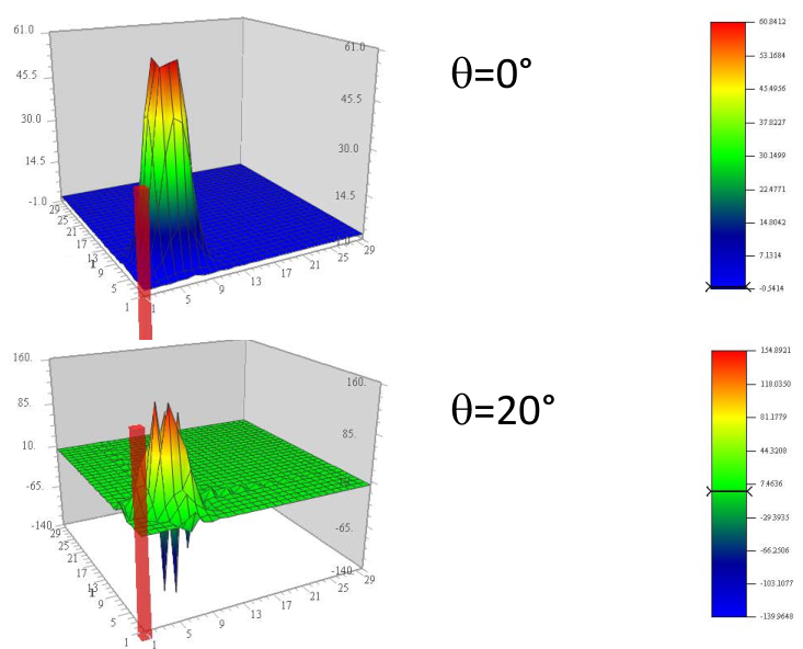
Refer to caption — Figure 2.4: Real parts of the potential energy matrix elements for INOY np interaction in $3S_{1}$ wave. The projection is made on Lagrange-Laguerre basis of 30 functions. The z-axis reflects the size of the matrix elements in MeV. In the upper figure matrix elements for the original potential, in the bottom figure for the CS transformed potential with $\theta=20^{\circ}$ .

2.3.1 The complex scaling operator

Numerous problems in quantum mechanics are related to isolated systems, which are subject to energy conservation. Usually this kind of problems can be reformulated in a time-independent frame by factoring out the time-dependent part of their wave-function. When considering non-relativistic dynamics a time-independent formalism leads to solve a generalized N-body Schrödinger equation with an eventually present inhomogeneous term:

(E-\widehat{H}_{0}-\sum_{i}\widehat{V}_{i})\Psi=I.

(2.97)

In the last equation $E$ is systems total energy, $\Psi$ its wave function, or at least its non-trivial part²² 2 As it will be demonstrated, it is possible to rewrite the problem in such a way that the wave function $\Psi$ contains only outgoing waves.. $H_{0}$ denotes kinetic energy operator, whereas $\widehat{V}_{i}$ denotes operators representing potential energy terms. For sake of simplicity one may express the total Hamiltonian as $\widehat{H}=\widehat{H}_{0}+\sum_{i}V_{i}.$ Eventually on the right hand of the last equation an inhomogeneous term $I$ is present. An inhomogeneous term appears in diverse scattering problems and may be straightforwardly related to an initial state, which for the problems related with a realistic experiment is supposed to be known a-priori (predefined by the experimental setup) and therefore represents a trivial part of the problem. In this case $\Psi$ represents wave function’s behavior in relation with a final state, describing distribution of the reaction products. Since the reaction products should evolve from the collision-center (closely localized area, where particles are supposed to hit each other), their distribution should be described by the outgoing spherical waves – waves evolving in all the directions from the collision area. The wave function $\Psi$ thus carries key information about the considered system, in particular in its far-asymptote information about the particle distribution after reaction takes place is encoded and thus is straightforwardly related with the experimental observables. The main asset of the complex scaling method is due to simple and efficient treatment of the outgoing waves.

Problems of finding bound or resonant states, particle collisions or reactions due to an impact of an external probe might be presented in the general form of eq. (2.97). Nevertheless direct solution of the last equation presents a formidable task already for a three-particle systems. Additional complications arise due to the fact that most of the computational methods in quantum mechanics have been developed for the Hermitian operators. However the physical Hamiltonians are Hermitian only when they operate on bounded (square integrable) functions. Wave functions describing resonant states or particle collisions does not meet the last criteria. Nevertheless as will be demonstrated here, an extension of the variational principle and of the other well-known theorems in quantum mechanics to the non-Hermitian operators can be made by carrying out similarity transformations $\widehat{S}$ , which converts outgoing scattered waves, $\phi^{out}$ , into square integrable functions. That is,

E\left(\widehat{S}\Psi\right)-\left(\widehat{S}\widehat{H}\widehat{S}^{-1}\right)\left(\widehat{S}\Psi\right)=\widehat{S}I,

(2.98)

such that

\widehat{S}\phi^{out}(r\rightarrow\infty)\rightarrow 0,

(2.99)

and $\widehat{S}\phi^{out}(r)$ is in the Hilbert space although $\phi^{out}(r)$ is not. The complex-scaling operator, to be defined below, is only one example of a vast set of similarity transformations for which the last equation is satisfied. However the simplicity of the complex-scaling operator and its conformity with the existing numerical methods makes it unexcelled in the practical applications.

The complex-scaling (CS) operator is defined as

\widehat{S}=\exp(i\theta r\frac{\partial}{\partial r}),

(2.100)

such that

\widehat{S}f(r)=f(re^{i\theta}).

(2.101)

As already mentioned, of particular interest is the action of this operator on the outgoing scattered waves

\widehat{S}\phi^{out}(r\rightarrow\infty)\propto\exp(ikre^{i\theta}),

(2.102)

in this equation $k$ denotes the scattering momentum.

CS transformation of the Hamiltonian is also rather trivial. For a sake of clarity, and without loss of generality, let us consider an one-dimensional radial Hamiltonian. When the potential is dilation analytic, the complex-scaled Hamiltonian is simply:

	$\displaystyle H_{l}^{\theta}$	$\displaystyle=$	$\displaystyle\widehat{S}\widehat{H}\widehat{S}^{-1}$		(2.103)
		$\displaystyle=$	$\displaystyle-\frac{\hbar^{2}}{2\mu}\frac{d^{2}}{e^{2i\theta}dr^{2}}+\frac{\hbar^{2}}{2\mu}\frac{l(l+1)}{e^{2i\theta}r^{2}}+V(re^{i\theta}).$		(2.104)

From the last expression it follows that the kinetic energy operator is simply scaled by the factor $e^{-2i\theta}$ after the CS transformation is applied:

T_{ij}^{\theta}=\frac{1}{e^{2i\theta}}T_{ij}.

(2.105)

Calculation of the potential energy matrix is more complicated, but still rather standard. For the local potential one has:

V_{ij}^{\theta}=\left\langle f_{i}\left|\widehat{S}\widehat{V}\widehat{S}^{-1}\right|f_{j}\right\rangle=\int_{0}^{\infty}f_{i}(r)V(re^{i\theta})f_{j}(r)dr,

(2.106)

If the potential is non-local $V(r,r\prime)$ :

V_{ij}^{\theta}=\int_{0}^{\infty}e^{i\theta}f_{i}(r)V(re^{i\theta},r^{\prime}e^{i\theta})f_{j}(r^{\prime})drdr^{\prime}.

(2.107)

One may refer to the section 2.5.1 for a more detailed discussion on the CS transformation of the potential energy.

2.3.2 Bound states

In quantum mechanics, bound states are defined as localized solutions of the Schrödinger equation, without a source term $I\equiv 0$ . These states appear as the poles of the S-matrix on a positive imaginary momentum axis $k_{bs}=i\left|k_{bs}\right|=\sqrt{\frac{mE_{bs}}{\hbar^{2}}}$ (see figure 2.5). Bound state wave functions in their asymptotes involve only outgoing waves and thus:

\phi_{bs}(r\rightarrow\infty)\propto\exp(ik_{bs}r)=\exp(-\left|k_{bs}\right|r).

(2.108)

By virtue of the last equation, bound state wave functions are exponentially bound and belong to the Hilbert space. The action of the CS operator on a bound state wave function gives:

\widehat{S}\phi_{bs}(r\rightarrow\infty)\propto\exp(-\left|k_{bs}\right|re^{i\theta})=\exp(-\left|k_{bs}\right|r\cos\left(\theta\right))\exp(-i\left|k_{bs}\right|r\sin\left(\theta\right)).

(2.109)

This function remains in the Hilbert space as long as a CS angle satisfy $mod(\theta-\pi/2,2\pi)<\pi/2$ ³³ 3 In practice it is convenient to limit the complex scaling angles to $0\leq\theta<\pi/2$ . Naturally one may solve CS Schrödinger equation for $\overline{\phi}_{bs}^{\theta}=\widehat{S}\phi_{bs}:$

E_{bs}\overline{\phi}_{bs}^{\theta}-\left(\widehat{S}\widehat{H}\widehat{S}^{-1}\right)\overline{\phi}_{bs}^{\theta}=0,

(2.110)

to determine bound state energies $E_{bs}$ and their wave function representations $\overline{\phi}_{bs}^{\theta}$ due to CS transformation. As long as CS angle satisfies the condition $mod(\theta-\pi/2,2\pi)<\pi/2,$ the last equation might be solved using techniques based on Hilbert space methods by expanding $\overline{\phi}_{bs}^{\theta}$ with a square integrable basis function set.

Obviously CS transformation does not bring any added value in solving bound state problem by itself, since the CS Schrödingers equation (2.110) is more complicated than a non-transformed one. After CS transformation the structure of a bound state wave function $\overline{\phi}_{bs}^{\theta}(r)$ becomes more complicated than its original image $\phi_{bs}(r)$ , gaining additional oscillating factor $\exp(-i\left|k_{bs}\right|r\sin\left(\theta\right))$ in the far asymptote. Nevertheless, as it will be demonstrated in the following, if one wish to apply CS method to solve scattering problems, CS images of the bound state wave functions are needed as an input in constructing initial state wave function. To this aim it turns to be numerically advantageous to solve eq. (2.110) and determine $\overline{\phi}_{bs}^{\theta}(r)$ , than try to construct $\overline{\phi}_{bs}^{\theta}$ using $\widehat{S}\phi_{bs}(r)$ relation.

2.3.3 Resonant states

In this study I will restrict to the resonant states related with the S-matrix poles appearing in the 4^th energy quadrant. Two-particle resonant state wave functions are defined by the outgoing wave solutions of the two-body Schrödinger equation. It is

\phi_{n}(r\rightarrow\infty)\propto\exp(ik_{n}^{res}r),

(2.111)

with $k_{n}^{res}=\sqrt{\frac{m}{\hbar^{2}}E_{n}^{res}}$ representing momentum of a resonant state $n$ . It is of particular interest to express an action of the complex scaling operator on a wave function of a resonant state:

	$\displaystyle\widehat{S}\phi_{n}^{res}(r$	$\displaystyle\rightarrow$	$\displaystyle\infty)\propto\exp(ik_{n}^{res}re^{i\theta})=\exp(i\left\|k_{n}^{res}\right\|re^{i\left(\theta-\vartheta^{res}\right)})$		(2.112)
		$\displaystyle=$	$\displaystyle\exp(i\left\|k_{n}^{res}\right\|r\cos\left(\theta-\vartheta^{res}\right))\exp(-\left\|k_{n}^{res}\right\|r\sin\left(\theta-\vartheta^{res}\right))$		(2.113)

Thus one may easily see that if the condition

\text{mod}(\theta-\vartheta^{res},2\pi)<\pi

(2.114)

is satisfied, the complex-scaled resonance wave functions become exponentially convergent.

It is of interest to see how a CS transforation affects the spectra of the Hamiltonian. According to the Aguilar, Balslev and Combes theorem [9], see fig. 2.6):

1.

The bound state poles remain unchanged under the transformation.
2.

The cuts are now rotated downward making an angle of $2\theta$ with a real axis.
3.

The resonant poles are “exposed” by the cuts once the “rotational angle” $\theta$ is greater than $-\frac{1}{2}Arg(E_{res})$ , where $E_{res}$ is the complex resonance energy.

It is easy to prove this theorem for the short-range potentials. In such a case, the asymptotic behavior of the scattering states is given by:

\phi^{scatt}(r\rightarrow\infty)=A(k)e^{-ikr}+B(k)e^{ikr}

(2.115)

where as usual center-of-mass kinetic energy (E) in terms of momentum (k) is expressed

E=\frac{\hbar^{2}}{2\mu}k^{2},

(2.116)

The energy takes any real positive value (provided that the threshold energy is taken as zero). The complex-scaled scattering states are given by

\widehat{S}\phi^{scatt}(r\rightarrow\infty)=A(k)e^{-ikre^{i\theta}}+B(k)e^{ikre^{i\theta}}.

(2.117)

One can see that these wave functions diverge if $\theta<\pi$ , since the real part of the exponential factor $e^{-ikre^{i\theta}}$ is positive. The only bounded non-divergent (not square integrable) functions are obtained when $k$ gets complex values,

k=\left|k\right|e^{-i\theta}

(2.118)

and therefore (when the threshold is taken as the zero reference energy)

E=\left|E\right|e^{-i2\theta}

(2.119)

According to the Aguilar, Balslev and Combes theorem [9] (ABC theorem), in order to find the resonant states one should simply solve an eigenvalue problem for a complex Hamiltonian:

H_{l}^{\theta}\widetilde{\phi}_{n}^{\theta}(r)=E_{n}^{\theta}\widetilde{\phi}_{n}^{\theta}(r),

(2.120)

keeping in mind that the resonant eigenvalues are “exposed” by the cuts of the rotated continuum states, that is $\theta>-\frac{1}{2}Arg(E_{R})$ .

The complex analog to the variational principle provides the formal justification to the use of the computational techniques that originally were developed for the bound state problems. The Rayleigh quotient

E_{n}^{\theta}=\frac{(\phi\left|H_{l}^{\theta}\right|\phi)}{(\phi\left|\phi\right)}

(2.121)

provides a stationary approximation to the true complex eigenvalue $E_{n}^{\theta}$ when $\phi$ is a c-normalizable eigenfunction of $H_{l}^{\theta}$ , which is close to exact solution $\widetilde{\phi}_{n}^{\theta}(r).$ This means that the calculated eigenvalues, corresponding to some resonant state, will stabilize around the exact solution without providing any bound (upper, lower) for the eigenenergy.

In practice, the convergence of the calculated resonance eigenvalues might be improved by either increasing the size of the eigenfunction basis (or density of the wave-function discretization points), or by increasing the complex scaling angle beyond its critical value $\theta=-\frac{1}{2}Arg(E_{R})$ ⁴⁴ 4 It is important to note, as will be demonstrated in the following section that there may exist potential depending maximal value of the CS angle $\theta p,$ beyond which one is not able to realize CS transformation of the potential.. The physical resonance eigenvalues frequently appear close to the thresholds and therefore the values of $\left|k_{n}^{res}\right|$ in eq.(2.113) are usually small, resulting slow decaying exponent for the CS resonant wave functions. At the same time, due to the presence of the exponent $\exp(i\left|k_{n}^{res}\right|r\cos\left(\theta-\vartheta^{res}\right))$ these asymptotes might be strongly oscillating. This demonstrates that much of the care should be taken in describing the far-extending parts of the resonant wave functions.

These general developments might be easily extended to the problems related with a few-particle resonant states. One must simply keep in mind that a few-particle resonance wave function might involve more than one outgoing wave, related with a presence of more than one scattering threshold. Therefore very similar condition, as one formulated for a 2-body case in eq.(2.114), should be validated relative to each open threshold. Furthermore one should be aware of the possible appearance of the discretized continuum pseudostates, associated with a presence of the resonant states in the multiparticle subsystems (see fig. 2.5). In the momentum manifold these pseudostates align along the lines starting from a resonant subsystem’s momentum and are bent by angle $\theta$ relative to the real axis.

2.3.4 Extended completeness relation

The complex eigenvalues obtained for a complex-scaled Hamiltonian have a very physical interpretation. In the work of K. Katō, B. Giraud et al. [13, 14, 15] the completeness relation of T. Berggren [40] has been proved for the complex scaled Hamiltonian solutions representing bound, resonant as well as single- and coupled-channel scattering states. This completeness relation can be formulated for the Cauchy integral contour in the momentum plane as demonstrated in fig. 2.5, as:

\mathbf{1}=\sum_{b}\left|\chi_{b}^{\theta}\right)\left(\chi_{b}^{\theta}\right|+\sum_{r}^{n_{r}^{\theta}}\left|\chi_{r}^{\theta}\right)\left(\chi_{r}^{\theta}\right|+\int_{L_{k}^{\theta}}dk_{\theta}\left|\chi_{k_{\theta}}\right)\left(\chi_{k_{\theta}}\right|,

(2.122)

here $\chi_{b}^{\theta}$ and $\chi_{r}^{\theta}$ are the complex scaled bound and resonant state wave-functions respectively. Only the resonant states encircled by a semicircle rotated by an angle $\theta$ must be considered. Remaining continuum states $\chi_{k}^{\theta}$ are located on the rotated momentum axis $L_{k}^{\theta}$ (see figure 2.5). One should mention that the definition of the complex scaled bra- and ket-states for a non-Hermitian $H^{\theta}$ is different from one defined for Hermitian Hamiltonians. For the complex scaled Hamiltonian $H^{\theta}$ one express a bra-state as bi-conjugate solution of the equivalent ket-state. In practice, for the discrete (resonant and bound) states we can use the same wave functions for the bra- and ket-states; for the continuum states, the wave function of a bra-state is given by that of the equivalent ket-state divided by the S-matrix.

Using the former completeness relation, one may construct the complex scaled Green’s function as

\mathcal{G^{\theta}}(E,\mathbf{r},\mathbf{r^{\prime}})=\sum_{b}\frac{\left|\chi_{b}^{\theta}(\mathbf{r})\right)\left(\chi_{b}^{\theta}(\mathbf{r^{\prime}})\right|}{E-E_{b}}+\sum_{r}^{n_{r}^{\theta}}\frac{\left|\chi_{r}^{\theta}(\mathbf{r})\right)\left(\chi_{r}^{\theta}(\mathbf{r^{\prime}})\right|}{E-E_{r}}+\int_{L_{k}^{\theta}}dk_{\theta}\frac{\left|\chi_{k_{\theta}}(\mathbf{r})\right)\left(\chi_{k_{\theta}}(\mathbf{r^{\prime}})\right|}{E-E_{\theta}},

(2.123)

where $E_{b}$ and $E_{r}=(E_{R}-\frac{i}{2}\Gamma)$ are the energy eigenvalues of the bound and relevant resonant states respectively. Variables $\mathbf{r}$ reflect all the internal coordinates of the multiparticle system under consideration.

Figure 2.6: Schematic representation of the eigenvalues of the complex scaled Hamiltonian,

H^{\theta}

, according to the theorem of Aguilar, Balslev and Combes [9]. For a two-body system (left panel) bound states are obtained as negative real energy eigenvalues, continuum-pseudostates are rotated by angle

2\theta

, resonant states inside

2\theta

branch may also be obtained. For a many-body system (right panel) several rotated continuum branches exist associated with bound and resonant thresholds in its subsystems.

For the sake of simplicity, the contour depicted in the figure 2.5 represents the simplest 2-body case. Still all of the presented relations remain valid for the many-body system; one only should keep in mind that the obtained spectra may have a much more complicated structure. Following the ABC theorem [9] the eigenvalues of the complex-scaled two-body Hamiltonian, which are associated with the bounded wave function, splits into three categories: bound state eigenvalues situated on the negative horizontal energy axis, the pseudo-continuum states scattered along the positive energy axis rotated by angle $2\theta$ and eigenvalues representing the resonant states whose eigenergies satisfies the relation - $arg(E)<2\theta$ (see left panel of figure 2.6). For the many-body system, bound states will be situated on the horizontal part of the energy axis, situated below the lowest systems separation into multiparticle clusters threshold (see figure 2.6). Pseudo-continuum states will scatter along the $2\theta$ -lines projected from each possible separation threshold. In addition, one will have $2\theta$ -lines projected from the ”resonant thresholds”, where one or more sub-clusters are resonant. Finally, many-body resonance eigenvalues will manifest as discrete points inside the semicircle making angle $2\theta$ with real energy axis and derived from the lowest threshold.

2.3.5 Reactions due to external probes

There is a vast group of problems in physics where a system is initially in a bound state and is excited to the continuum by a perturbation. In particular, it concerns reactions led by electro-magnetic and weak probes. For these reactions one is led to evaluate the strength (or the response) function, which in the lowest order perturbation theory is provided by

S(E)=\sum_{\nu}\left|\left\langle\Psi_{\nu}\left|\hat{O}\right|\Psi_{0}\right\rangle\right|^{2}\delta(E_{\nu}-E_{0}-E),

(2.124)

where $\hat{O}$ is the perturbation operator which induces a transition from a bound-state $\Psi_{0},$ with a ground-state energy $E_{0}$ , to a state $\Psi_{\nu}$ with an energy $E_{\nu}$ . Both wave functions are solutions of the same Hamiltonian : $H$ . The energy is measured from some standard value, e.g., a particle-decay threshold energy. When the excited state is in the continuum, the label $\nu$ is continuous and the sum must be replaced by an integration. The final state wave function $\Psi_{\nu}$ may have complicate asymptotic behavior in configuration space if it represents a continuum state. On the other hand the expression may be rewritten by avoiding summation over the final states

	$\displaystyle S(E)$	$\displaystyle=$	$\displaystyle\left\langle\Psi_{0}\left\|\hat{O}^{{\dagger}}\delta(H-E_{\nu})\hat{O}\right\|\Psi_{0}\right\rangle$		(2.125)
		$\displaystyle=$	$\displaystyle-\frac{1}{\pi}Im\left\langle\Psi_{0}\left\|\hat{O}^{{\dagger}}G(E_{\nu}+i\varepsilon)\hat{O}\right\|\Psi_{0}\right\rangle=-\frac{1}{\pi}Im\left\langle\Psi_{0}\left\|\hat{O}^{{\dagger}}\right\|\Phi_{\nu}\right\rangle,$		(2.126)

with

(H-E_{\nu})\Phi_{\nu}=\hat{O}\Psi_{0}.

(2.127)

The right hand side of the former equation is compact, damped by the bound-state wave function $\Psi_{0}$ . The wave function $\Phi_{\nu}$ in its asymptote will contain only outgoing waves. Therefore the last inhomogeneous equation might be readily solved using complex scaling techniques

(H^{\theta}-E_{\nu})\overline{\Phi}_{\nu}^{\theta}=\hat{O}^{\theta}\Psi_{0}^{\theta}.

(2.128)

To do so, one should construct the CS inhomogeneous term, present in the right hand side of the last equation. A practical way to obtain complex-scaled bound state wave functions $\Psi_{0}^{\theta}$ is to solve bound state problem for the complex-scaled Hamiltonian

(H^{\theta}-E_{0})\Psi_{0}^{\theta}=0,

(2.129)

as explained in the section 2.3.2.

In order to solve eq. (2.128), one projects it on a chosen square-integrable basis ( $f_{i}$ ) employed to expand wave function $\Psi_{0}^{\theta}$ :

\Psi_{0}^{\theta}(r)=\sum_{i}c_{i}^{\theta}f_{i}(r),

(2.130)

where naturally the expansion coefficients $c_{i}^{\theta}$ are complex numbers. This procedure leads to a standard linear algebra problem:

\left(\left[E\right]-\left[\hat{H^{\theta}}\right]\right)c^{\theta}=w^{in,\theta}.

(2.131)

here $\left[E\right],\left[\hat{H^{\theta}}\right]$ are the same matrices as for CS resonances problem, representing projection of norm matrix and Hamiltonian. Vector $w^{in,\theta}$ represents projection of the inhomogenious term $\hat{O}^{\theta}\Psi_{0}^{\theta}$ on a chosen basis $f_{i}(r)$ .

There are two distinct ways to solve the linear algebra problem eq. (2.131) and evaluate the associated strength function eq. (2.126). The first one, and probably the most practical one, relies on the direct solution of the linear algebra problem. Once the coefficients $c_{i}^{\theta}$ are obtained, it makes no difficulty to calculate the strength function of eq. (2.126):

S(E)=-\frac{1}{\pi}Im\sum_{i}c_{i}^{\theta}w_{i}^{in,\theta}.

(2.132)

One may keep in mind that complicated few-particle problems may lead to linear algebra problems of very considerable size, where Hamiltonian matrix largely exceeds storage capacities of the available hardware. To confront this problem, iterative linear algebra methods exist [41], which allows to find the solution by avoiding storage of the matrix.

Complex scaled Green’s function method

Alternative solution of a linear algebra problem eq. (2.131) relies on the spectral expansion, widely employed in the works [13, 16, 17, 18, 19, 20]. In this case, the solution of the linear algebra problem is expanded in the eigensolutions $\widetilde{\phi}_{i}^{\theta}(r)$ of the Hamiltonian matrix $\left[\hat{H^{\theta}}\right]$ :

	$\displaystyle\overline{\Phi}_{\nu}^{\theta}(\mathbf{r})$	$\displaystyle=$	$\displaystyle\sum_{i=1}^{N}a_{i}\widetilde{\phi}_{i}^{\theta}(r)$		(2.133)
	$\displaystyle a_{i}$	$\displaystyle=$	$\displaystyle\frac{\left(\widetilde{\phi}_{i}^{\theta}(r)\right.\left\|w^{in,\theta}\right)}{E-E_{i}^{\theta}}$		(2.134)

Finally, strength function is obtained via:

S(E)=-\frac{1}{\pi}Im\left\langle\Psi_{0}^{\theta}\left|(\hat{O}^{{\dagger}})^{\theta}\right|\overline{\Phi}_{\nu}^{\theta}\right\rangle.

(2.135)

By inserting the last relation into the eq. (2.126), one finally gets:

$\displaystyle S(E)$	$\displaystyle=$	$\displaystyle S_{b}(E)+S^{\theta}_{r}(E)+S^{\theta}_{k}(E),$	(2.136)
$\displaystyle S_{b}(E)$	$\displaystyle=$	$\displaystyle-\frac{1}{\pi}Im\sum_{b}\frac{\left(\Psi_{0}^{\theta}\right\|(\hat{O}^{\dagger})^{\theta}\left\|\chi_{b}^{\theta}\right)\left(\chi_{b}^{\theta}\right\|\hat{O}^{\theta}\left\|\Psi_{0}^{\theta}\right)}{E-E_{b}},$	(2.137)
$\displaystyle S^{\theta}_{r}(E)$	$\displaystyle=$	$\displaystyle-\frac{1}{\pi}Im\sum_{r}^{n_{r}^{\theta}}\frac{\left(\Psi_{0}^{\theta}\right\|(\hat{O}^{\dagger})^{\theta}\left\|\chi_{r}^{\theta}\right)\left(\chi_{r}^{\theta}\right\|\hat{O}^{\theta}\left\|\Psi_{0}^{\theta}\right)}{E-E_{r}},$	(2.138)
$\displaystyle S^{\theta}_{k}(E)$	$\displaystyle=$	$\displaystyle-\frac{1}{\pi}Im\int_{L^{\theta}_{k}}\frac{\left(\Psi_{0}^{\theta}\right\|(\hat{O}^{\dagger})^{\theta}\left\|\chi_{k_{\theta}}\right)\left(\chi_{k_{\theta}}\right\|\hat{O}^{\theta}\left\|\Psi_{0}^{\theta}\right)}{E-E_{\theta}}.$	(2.139)

In practice (numerical solution), one works with a finite basis; then, the last term containing integration is replaced by a sum running over all the complex eigenvalues, representing continuum pseudo states. All the eigenvalues are obtained as solutions of the complex scaled Hamiltonian with a pure outgoing wave boundary condition – exponentially converging ones due to the complex scaling.

The obtained total strength function $S(E)$ should be independent of the angle $\theta$ , employed in the calculation. Furthermore the strength function component $S_{b}(E)$ as well as its partial components due to contribution of the separate bound states are also independent of $\theta$ . The partial components of the $S^{\theta}_{r}(E)$ , corresponding to narrow resonant states, also turn to be independent of $\theta$ , as long as the angle $\theta$ is large enough to encircle these resonances. However if a resonance is large enough and is not encircled by the contour $L^{\theta}_{k}$ its contribution to the strength function is reabsorbed by the pseudo-continuum states in the $S^{\theta}_{k}(E)$ term. This feature has been clearly demonstrated in the ref. [17] for a chosen 2-body example.

Another instructive example is provided in figure 2.7, comparing contributions to E1 strength function by a narrow and broad resonances. One may see that narrow resonance carries most of the strength. Contribution of the broad resonances is comparable to the one of the continuum. Furthermore, while the full strength function is a positive quantity, the partial contributions of the resonant or continuum states may contain regions in energy with negative contribution to the total strength function. However once all the partial contributions are summed positive value of the total strength function should be recovered.

Relation (2.136) offers an unique feature to separate the contributions of the resonant and bound states in the strength function, providing clear physical interpretation of the various components in the strength function.

Figure 2.7: Dipole-response functions (black line) with separated contribution of the resonance obtained via complex scaling (red line). In the left panel results are presented for a potential containing a narrow resonance at

E^{res}=0.48-0.064i

, whereas right panel is for a potential supporting resonance at

E^{res}=6.56-3.9i

2.4 Complex-scaling method for the collisions

In the previous sections I have demonstrated how efficient CS method could be in handling problems dominated by the outgoing wave functions. Particle collisions turns to be slightly more complicated case, since their wave functions contain the incoming waves $\Psi_{a}^{in}$ , associated with the initial projectile-target states, and highly untrivial outgoing waves $\Psi_{a^{\prime}}^{out}$ representing various possible reaction channels:

\Psi^{scatt}(k_{a})_{\rho\rightarrow\infty}=\Psi_{a}^{in}(k_{a})+\sum\limits_{a^{\prime}}f_{a^{\prime}a}(k_{a})\Psi_{a^{\prime}}^{out}(k_{a})

(2.140)

Nevertheless, once again, the problem might be reformulated in a way suitable for CS method, as have been demonstrated for the first time by J. Nuttal and H.I. Cohen [7].

2.4.1 Scattering, two-body problem

Short range, exponentially bound, interactions

The idea of J. Nuttal and H.I. Cohen [7] can be briefly formulated as follows. The Schrödinger equation is recast into its inhomogeneous (driven) form by splitting the wave function into the sum $\Psi(r)=$ $\Psi^{out}(r)+\Psi^{in}(r)$ , where an incident (free) $\Psi^{in}(\mathbf{r})=\exp(i\mathbf{k}\cdot\mathbf{r})$ wave is separated. A remaining untrivial part of the systems wave function $\Psi^{out}(\mathbf{r})$ describes scattered waves and may be found by solving a second-order differential equation with an inhomogeneous term:

[E-\hat{H_{0}}-V(\mathbf{r})]\Psi^{out}(\mathbf{r})=V(\mathbf{r})\Psi^{in}(\mathbf{r}).

(2.141)

The scattered wave is represented in the asymptote by an outgoing wave $\Psi^{out}\sim\exp(ikr)/r,$ where $k=\sqrt{2\mu E}/\hbar$ is the wave number for the relative motion. If one scales all the particle coordinates by a constant complex factor, i.e. $r_{i}^{\theta}=e^{i\theta}r_{i}$ with $Im(e^{i\theta})>0$ , the corresponding scattered wave $\overline{\Psi}^{out,\theta}(\mathbf{r})$ will vanish exponentially $\sim\exp(-kr\sin\theta)$ as particle separation $r$ increases. Moreover if the interaction is of short range – exponentially bound with the longest range $\eta^{-1}$ – then after complex scaling the right hand side of eq. (2.141) also tends to zero at large $r$ , if :

\tan\theta<\eta/k.

(2.142)

From here we introduce the notation $f^{\theta}(r)=f(re^{i\theta})$ for the complex-scaled functions. The complex scaled driven Schrödinger equation becomes:

[E-e^{-i2\theta}\hat{H_{0}}-V^{\theta}(\mathbf{r})]\overline{\Psi}^{out,\theta}(\mathbf{r})=V^{\theta}(\mathbf{r})\overline{\Psi}^{in,\theta}(\mathbf{r}).

(2.143)

If the condition in eq. (2.142) is satisfied, the former inhomogeneous equation may be solved by using a compact basis to expand $\overline{\Psi}^{out,\theta}(\mathbf{r})$ , thus by employing standard bound-state techniques:

\overline{\Psi}^{out,\theta}(\mathbf{r})=\sum_{i=1}^{N}c_{i}^{\theta}f_{i}(r),

(2.144)

with $c_{i}^{\theta}$ denoting complex expansion coefficients, while $f_{i}(r)$ is a function from the conveniently chosen compact basis. After projecting equation on the basis states $f_{i}(r)$ , as previously, one gets linear algebra problem to be solved:

\left(\left[E\right]-\left[\hat{H^{\theta}}\right]\right)c^{\theta}=v^{in,\theta},

(2.145)

here $\left[E\right],\left[\hat{H^{\theta}}\right]$ are the same square matrices representing projection of norm matrix and Hamiltonian, whereas vector $v^{in,\theta}$ denotes projection of the inhomogenious term $V^{\theta}(\mathbf{r})\overline{\Psi}^{in,\theta}(\mathbf{r})$ on a chosen basis $f_{i}(r)$ .

As discussed in a previous section, there are two mathematically equivalent ways to solve the last set of linear equations in order to obtain vector $c^{\theta}$ , which contains coefficients $c^{\theta}_{i}$ representing projection of the function $\overline{\Psi}^{out,\theta}(\mathbf{r})$ :

•

Solve linear-algebra problem, formulated in eq. (2.145)

•

Use spectral expansion of the last equation into eigensolutions of matrix $\left[\hat{H^{\theta}}\right]$ . In this case:

	$\displaystyle\overline{\Psi}^{out,\theta}(\mathbf{r})$	$\displaystyle=$	$\displaystyle\sum_{i=1}^{N}a_{i}\widetilde{\phi}_{i}^{\theta}(r)$		(2.146)
	$\displaystyle a_{i}$	$\displaystyle=$	$\displaystyle\frac{\left(\widetilde{\phi}_{i}^{\theta}(r)\right.\left\|v^{in,\theta}\right)}{E-E_{i}^{\theta}}.$		(2.147)

There are no need to repeat the arguments of the previous section reflecting the advantages of two different methods. It worths only mentioning that spectral expansion formalism allows to use the same dataset of the eigensolutions to obtain results on the bound, resonant states as well as particle collisions or reactions due to the external probes.

From the obtained CS representation of the scattered wave function $\overline{\Psi}^{out,\theta}(\mathbf{r})$ there are three ways to extract scattering observables.

•

The most straightforward way is based on the analysis of the asymptotic behavior of the outgoing waves. In this case the scattering amplitude $f_{k}(\hat{r})$ is extracted in a similar way as the asymptotic normalization coefficient from the bound-state wave function, that is, by matching asymptotic behavior of the solution:

\overline{\Psi}^{out,\theta}(\mathbf{r\rightarrow\infty})=f_{k}(\widehat{k})e^{-i\theta}\exp(ikre^{i\theta})/r.

(2.148)

•

Another well known alternative is to use the integral relations, which one gets after applying the Green’s theorem [21, 22, 42]. For a simple case of two-particle scattering this gives:

	$\displaystyle f_{k}(\widehat{k})$	$\displaystyle=$	$\displaystyle-\frac{1}{E_{cm}}e^{i3\theta}\int(\Psi^{in\ast})^{\theta}(\mathbf{r})V^{\theta}(\mathbf{r})\left[\overline{\Psi}^{out,\theta}(\mathbf{r})+\overline{\Psi}^{in,\theta}(\mathbf{r})\right]d^{3}r$		(2.149)
		$\displaystyle=$	$\displaystyle-\frac{1}{E_{cm}}e^{i3\theta}\int(\Psi^{in\ast})^{\theta}(\mathbf{r}){V^{\theta}}(\mathbf{r})\overline{\Psi}^{out,\theta}(\mathbf{r})d^{3}r-\frac{1}{E_{cm}}\int(\Psi^{in}(\mathbf{r}))^{\ast}V(\mathbf{r}){\Psi}^{in}(\mathbf{r})d^{3}r.$		(2.150)

Where $E_{cm}=\frac{\hbar^{2}k^{2}}{2\mu}$ is center-of-mass energy of the colliding particles. In the second relation one has separated the Born term, which may be evaluated without performing complex scaling. The $(\Psi^{in\ast})^{\theta}(\mathbf{r})$ term is obtained by applying complex-scaling operation on the bi-conjugate function $(\Psi^{in}(\mathbf{r}))^{\ast}$ . The radial part of the former function coincides with one of the $(\Psi^{in})^{\theta}(\mathbf{r})$ , whereas complex-conjugation is applied only on angular functions (spherical harmonics). Therefore manipulations involving bi-conjugate functions is straightforward.

If the spectral expansion is used, the scattering amplitude $f_{k}(\widehat{k})$ is obtained as a sum of the separate contributions: a Born term, contributions from bound, resonant and discretized continuum states obtained as eigensolutions of $\left[\hat{H^{\theta}}\right]$ .

•

Finally, the scattering phaseshifts may be extracted using continuum level density (CLD) formalism. One starts with the CLD definition:

\Delta(E)=-\frac{1}{\pi}\text{Im}\left(\text{Tr}[G(E)-G_{0}(E]\right),

(2.151)

where $G(E)=(E-H)^{-1}$ and $G_{0}(E)=(E-H_{0})^{-1}$ denote full and free Green’s functions, respectively. In principle, the former expression may be generalized to the scattering of two composit clusters. Then $H_{0}$ , besides the kinetic energy, should include interactions inside separate clusters, whereas $H$ includes all the interaction terms in two-cluster system. Thus CLD express the effect from the interactions connecting two clusters. When the eigenvalues of $H$ and $H_{0}$ are obtained approximately ( $\epsilon_{i}$ and $\epsilon_{i}^{0}$ respectively) within the framework including finite number of the basis functions (N), the discrete CLD is defined:

\Delta(E)_{N}=\sum_{i}\delta(E-\epsilon_{i})-\sum_{j}\delta(E-\epsilon_{j}^{0}).

(2.152)

The CLD is related to the scattering phaseshift as:

\Delta(E)=\frac{1}{\pi}\frac{d\delta(E)}{dE}

(2.153)

and thus one can inversely calculate the phaseshift ( $\delta$ ) by integrating the last equation obtained as a function of energy. These equations are difficult to apply for real Hamiltonians, as one will necessarily confront the singularities present in eqs. (2.151-2.152). However by using CS expressions for the Green’s functions, these singularities are avoided and replaced by the smooth Lorentzian functions. By plugging in CS Green’s function expression (2.123) into eq. (2.152) and after some simple algebra one gets:

\Delta(E)_{N}=\overline{\rho}_{N}^{\theta}(E)-\overline{\rho}_{0,N}^{\theta}(E)

(2.154)

and

$\displaystyle\overline{\rho}_{N}^{\theta}(E)$	$\displaystyle=$	$\displaystyle\sum_{b}^{n_{b}}\delta(E-E_{b})+\frac{1}{\pi}\sum_{r}^{n_{r}^{\theta}}\frac{Im(E_{r})}{\left[E-Re(E_{r})\right]^{2}+\left[Im(E_{r})\right]^{2}}$	(2.155)
	$\displaystyle+$	$\displaystyle\frac{1}{\pi}\sum_{k}^{N-n_{r}^{\theta}-n_{b}}\frac{Im(E_{k}^{\theta})}{\left[E-Re(E_{k}^{\theta})\right]^{2}+\left[Im(E_{k}^{\theta})\right]^{2}},$	(2.155)
$\displaystyle\overline{\rho}_{0,N}^{\theta}(E)$	$\displaystyle=$	$\displaystyle\frac{1}{\pi}\sum_{k}^{N}\frac{Im(E_{0,k}^{\theta})}{\left[E-Re(E_{0,k}^{\theta})\right]^{2}+\left[Im(E_{0,k}^{\theta})\right]^{2}}.$	(2.156)

In the last expression $E_{b},E_{r}$ and $E_{k}^{\theta}$ are the eigenvalues of the full CS Hamiltonian $H^{\theta}$ , representing bound, resonant and continuum states respectively. The term $\overline{\rho}_{0,N}^{\theta}$ is equivalent to $\overline{\rho}_{N}^{\theta}(E)$ only obtained for a free CS Hamiltonian $H_{0}^{\theta}$ ; this term contains only pseudo-continuum states $(E_{0,k}^{\theta})$ aligned along $2\theta$ -lines pointing out from the scattering thresholds (see figure 2.6).

By plugging the last two relations into eq. (2.153) and integrating it over the energy it is easy to get an expression for the phaseshifts:

\delta(E)=n_{b}\pi+\delta_{r}(E)+\delta_{k}(E),

(2.157)

with

	$\displaystyle\delta_{r}(E)$	$\displaystyle=$	$\displaystyle\sum_{r}^{n_{r}^{\theta}}\arctan\left[\frac{Re(E_{r})-E}{Im(E_{r})}\right],$		(2.158)
	$\displaystyle\delta_{k}(E)$	$\displaystyle=$	$\displaystyle\sum_{k}^{N-n_{r}^{\theta}-n_{b}}\arctan\left[\frac{Re(E_{k}^{\theta})-E}{Im(E_{k}^{\theta})}\right]-\sum_{k}^{N}\arctan\left[\frac{Re(E_{0,k}^{\theta})-E}{Im(E_{0,k}^{\theta})}\right]$		(2.159)

One may see that in these expression total phaseshift is obtained as a sum from the separated contributions of bound $n_{b}\pi$ , resonant $\delta_{r}(E)$ and continuum $\delta_{k}(E)$ states. According to the Levinson theorem bound states simply contribute in providing shift of the phase at the origin by $n_{b}\pi.$ Contribution of each resonant state to the phaseshift might be uniquely separated and they should not depend on the CS parameter $\theta$ as long as calculations are numerically converged. If the CS angle is able to ”expose” all the resonant states one gets also angle independent definition for the overall contribution of the continuum states to the total phaseshift. If some resonances are not exposed, their contribution to the phaseshift are compensated by the appropriate change in the continuum contribution $\delta_{k}(E)$ [43].

Presence of a long-range interaction

Let us consider a case where particle interaction apart short-range part includes an additional long-range term $V(\mathbf{r})=V_{s}(\mathbf{r})+V_{l}(\mathbf{r})$ , where $V_{s}(\mathbf{r})$ is exponentially bound, whereas $V_{l}(\mathbf{r})$ is long-ranged. CS method can be generalized to treat this problem if for the long-range term $V_{l}(\mathbf{r})$ the incoming wave solution $\Psi_{l}^{in}(\mathbf{r})$ is analytic and can be extended in to the complex r-plane [21, 44, 22]. Then one is left to solve the equivalent driven Schrödinger equation:

[E-e^{-i2\theta}\widehat{H_{0}}-V^{\theta}(\mathbf{r})]\overline{\Psi}_{s}^{sc}(\mathbf{r})=V^{\theta}_{s}(\mathbf{r})(\Psi_{l}^{in})^{\theta}(\mathbf{r}).

(2.160)

The inhomogeneous term on the right hand side of the former equation is moderated by the short-range interaction term, therefore it is exponentially bound if the condition eq.(2.142) is fulfilled by the short range potential $V_{s}(\mathbf{r})$ . Perfect example is related with a presence of the Coulomb interaction $V_{l}(\mathbf{r})=\frac{\hbar^{2}\eta}{\mu r}$ . For this case the incoming wave solution is well known and is usually expressed by the regular Coulomb functions $(\Psi_{l}^{in})^{\theta}(\mathbf{r})\equiv F_{l}(\eta,kre^{i\theta})$ .

One may establish a relation equivalent to the eq.(2.150) in order to determine the long-range-modified short-range interaction amplitude $f_{k,s}(\widehat{k})$ :

f_{k,s}(\widehat{k})=-\frac{1}{E_{cm}}e^{i3\theta}\int(\Psi_{l}^{in\ast})^{\theta}(\mathbf{r})V_{s}^{\theta}(\mathbf{r})\overline{\Psi}_{s}^{sc}(\mathbf{r})d^{3}r-\frac{1}{E_{cm}}\int(\Psi_{l}^{in}(\mathbf{r}))^{\ast}V_{s}(\mathbf{r}){\Psi}_{l}^{in}(\mathbf{r})d^{3}r.

(2.161)

The total scattering amplitude $f_{k}(\widehat{k})$ is a sum of a short-range one and the scattering amplitude due to the long-range term alone $f_{k,l}(\widehat{k})$ , known analytically:

f_{k}(\widehat{k})=f_{k,s}(\widehat{k})+f_{k,l}(\widehat{k}).

(2.162)

Short-range, exponentially non-bound, interactions

It is natural to pose a question about application of the CS method to describe scattering governed by short range interactions, decaying faster than 1/r ${}^{3},$ but which are not exponentially bound. From the formal point of view CS method, as described in two previous subsections, is not applicable for this case. On the other hand one may imagine solving a problem for a modified potential

\widetilde{V}(r)=f(r)V(r),

(2.163)

where $f(r)$ is some analytic function, which is very close to $1$ in the space region where the potential energy is important compared to the kinetic energy term, while this function makes $\widetilde{V}(r)$ vanish exponentially in the far asymptote. Depending on the choice of the function $f(r)$ one may rend scattering observables provided by the potential $\widetilde{V}(r)$ very close to ones obtained by the original potential $V(r)$ . On the other hand one has no formal obstacles to apply CS method in solving scattering problem related to the potential $\widetilde{V}(r)$ . Such a phenomenon has been already considered by J. Nutall [45]. One may see that if basis of exponentially bound functions is used to solve eq. (2.141) or eq. (2.160), in this case basis by itself partly fulfills function of the regulator $f(r)$ . Furthermore they have demonstrated that calculated scattering phases spiral around the exact value once one increases the basis size; it may approach very close to the exact value but when the basis is further increased the calculated phases start to recede from the exact ones continuing the spiral movement. In [46] it has been suggested to use Padé summation technique to gain accuracy from the approximately calculated phases which spiral around the exact value. For set of 2-body potentials they have demonstrated convergence of the Padé series and thus possibility to get very accurate evaluation of the scattering phaseshifts.

2.5 Example of the solution on a finite grid

To test the applicability of our approach we consider a system of two nucleons with a mass $\frac{\hbar^{2}}{m}=41.47$ MeV.fm², where the strong part of the nucleon-nucleon (NN) interaction is described by the spin-dependent S-wave MT I-III potential, formulated in [47] and parameterized in [48]:

V_{S}(r)=-A_{S}{\exp(-1.55r)\over r}+1438.72{\exp(-3.11r)\over r},

(2.164)

where $V_{S}(r)$ is in MeV and $r$ is in fm units. The attractive Yukawa strength is given by $A_{s=0}=-513.968$ MeV.fm and $A_{s=1}=-626.885$ MeV.fm for the two-nucleon interaction in spin singlet and triplet states respectively.

MT I-III potential has been chosen for two reasons. On one hand it is a widely employed potential for which accurate benchmark calculations exist. On the other hand this potential, being a combination of the attractive and repulsive Yukawa terms, reflects well the structure of the realistic nucleon-nucleon interaction: it is strongly repulsive at the origin but posses a narrow attractive well situated at $r\approx 1$ fm. Note that many numerical techniques fail to treat potentials like MT I-III, which include a repulsive core.

We have first considered a two-body case. In figure 2.8 we present our results for the NN ¹S₀ phaseshifts at $E_{cm}=$ 1 MeV. Two calculation sequences have been performed by forcing $\overline{\psi}_{l}^{sc}$ to vanish at the border of the numerical grid set at $r_{max}=50$ fm (in red) and $r_{max}=100$ fm (in blue) respectively, whereas the complex scaling angle $\theta$ has been chosen to be 10^∘ (dashed lines) and 30^∘ (solid lines). The phaseshifts are extracted by calculating logarithmic derivative of the wave function at a given distance and adjusting it to proper asymptotic behavior, including complex scaled Bessel or Coulomb functions. As one can see, the extracted phaseshifts oscillate with $r$ . This oscillatory behavior is due to the premature enforcement of $\overline{\psi}_{l}^{sc}(r)$ to vanish at the border of the grid $r_{\max}$ . The phaseshifts extracted close to $r_{\max}$ are strongly affected by the cut-off and are thus not reliable. The amplitude of the close-border oscillations is sizeably reduced by either increasing $r_{\max}$ or $\theta$ , i.e. by reducing the sharpness of the numerical cut-off. The extracted phaseshifts corresponding to the calculation with $r_{\max}=100$ fm and $\theta=$ 30^∘ are stable in a rather large window, which starts at $r\sim 5$ fm (right outside the interaction region) and extends up to $r\sim 70$ fm. Beyond this value the effect due to cut-off sets in. In the stability region the extracted phaseshifts agree well with the ”exact” results (dotted line), obtained by solving scattering problem using the standard (i.e. not complex rotated) boundary condition technique.

In figure 2.9 we have compared the NN ¹S₀ phaseshifts at different energies – $E_{cm}$ = $1$ , $5$ and $50$ MeV – by fixing $r_{\max}=100$ fm and $\theta$ =10^∘. One can see that when increasing the energy, the effect of the cut-off reduces, sizeably improving the stability of the extracted phaseshifts. The inclusion of the repulsive Coulomb term does not have any effect on the quality of the method.

One may improve considerably the accuracy of the phaseshifts by using the integral relation given in eq. (2.150). The results are displayed in tables 2.1, 2.2 and in figure 2.10. The phaseshifts converge to a constant value by either increasing the cut-off radius r_max or the complex rotation angle. A spectacular accuracy of five digits is easily reached. One should notice however that the use of very large values of $\theta$ should be avoided, due to the fact that the function $\overline{\psi}_{l}^{sc}(r)$ as well as the complex scaled potential $V(re^{i\theta})$ might become very steep and rapidly oscillating, see the discussion in the next section. At higher energy, the function $\overline{\psi}_{l}^{sc}(r)$ vanishes faster and thus one may easily achieve convergence by employing smaller values of r_max and/or $\theta$ .

Table 2.1: Calculation of the scattering phaseshifts using integral expressions at

E_{cm}=

1 MeV

	MT I-III				MT I-III+Coulomb
$r_{max}$ (fm)	5^∘	10^∘	30^∘	50^∘	5^∘	10^∘	30^∘	50^∘
10	44.420	49.486	55.790	56.676	33.999	36.390	41.528	43.805
25	34.704	44.211	62.654	63.743	24.772	34.910	50.693	50.698
50	56.812	61.083	63.482	63.512	39.895	46.546	50.487	50.491
100	66.502	63.822	63.512	63.512	55.463	50.811	50.491	50.491
150	62.497	63.485	63.512	63.512	49.317	50.474	50.491	50.491
exact	63.512				50.491

Table 2.2: Calculation of the scattering phaseshifts using integral expressions at

E_{cm}=

50 MeV

$r_{max}$ (fm)	MT I-III				MT I-III+Coulomb
	3^∘	5^∘	10^∘	30^∘	3^∘	5^∘	10^∘	30^∘
10	19.400	19.719	19.923	19.605	19.795	20.245	20.610	20.313
25	20.788	20.135	20.027	20.032	21.530	20.864	20.755	20.760
50	20.014	20.026	20.027	20.027	20.734	20.754	20.755	20.755
100	20.027	20.027	20.027	20.027	20.755	20.755	20.755	20.755
exact	20.027				20.755

2.5.1 General remarks about the complex scaling method

Spectral decomposition vs solution of the linear equation

As demonstrated in ref. [21], and briefly discussed in the section 2.3.5, there are two approaches to solve linear algebra problems, arising from the solution of a system of differential equations with an inhomogenious term, as generalized in eq. (2.97). They are: direct solution of the linear algebra problem or the method based on the spectral expansion of the linear algebra matrix. These two methods are fully equivalent, if accurately solved they provide results which coincide up to numerical round-off error.

It should be noted that a full spectral decomposition of the $H^{\theta}$ is required to express CS Green’s function in eq. (2.123) and to evaluate the scattering amplitudes. The scattering amplitude, except in the case of resonant scattering, is not determined by one or a few dominant eigenvalues⁵⁵ 5 One should notice however, if one tries to approximate the phaseshifts using only few eigenvalues, which are closest to the scattering energy, then the CLD formalism may provide better convergence than the relations (2.153-2.155).. This may turn out to be a crucial obstacle in applying CS Green’s function method in studying many-body systems, since the resulting algebraic eigenvalue problem becomes too large to be fully diagonalized. In this case the original prescription of J. Nuttall et al., based on direct solution of the linear algebra problem, turns to be strongly advantageous. The last prescription requires solution of the linear algebra problem eq.(2.145) at chosen energy points, allowing one to solve a resulting large-scale problem by iterative methods (requiring no explicit storage of the matrix elements).

On the other hand CS Green’s function formalism provides clear physical interpretation of the scattering observables in terms of bound, resonant and continuum states. Furthermore, the same input of eigenvalues and eigenvectors may be used to approximate CS Green’s function expression and then describe different processes in a chosen N-body system: bound states, resonant states, particle collisions or reactions induced by an external perturbations. In such a way a solid framework may be constructed to study correlations between the different physical observables.

CLD versus integral relation

Figure 2.11: Comparison of the absolute errors in extracting S-wave phaseshifts by using CLD and the integral relation formalisms. Results for four different energies are compared as a function of the Lagrange-Laguerre basis functions used to perform the calculations. Complex scaling angle has been set to

\theta=15^{\circ}

One disposes also three principally different methods to extract the scattering phaseshifts: by analyzing the shape of the wave function’s asymptote, employing integral relation or relation based on CLD expression. I would not discuss in detail the first method, success of it strongly depends on the choice of the wave function’s region to extract phaseshifts and thus it strongly relies on the skillfulness of a person performing calculations. One may simply recall from the discussion in a previous section that extraction region should be chosen beyond the range of the interaction, where a free asymptote is reached. The very far asymptote is neither suitable in numerical calculations, since the CS wave function is very small and thus strongly affected by the numerical inaccuracies.

On the other hand integral relations, like ones formulated in eq. (2.150-2.161), as well as CLD formalism provide the ready recipes to extract phaseshifts. Still accuracy of the two methods is quite different. In the figure 2.11 I present calculated S-wave phaseshifts for the potential consisting of two Yukawa functions

V(r)=678.097\frac{\exp(-2.54922r)}{r}-166.032\frac{\exp(-0.679864r)}{r},

(2.165)

and aiming to describe n-³H scattering, by setting a reduced mass of the system to $\frac{\hbar^{2}}{2\mu}=27.647$ MeV.fm. In the last expression the overall potential is expressed in units of MeV, whereas the distances are measured in fm units.

In these figures the absolute errors in the extracted phaseshifts are presented as a function of Lagrange-Laguerre basis functions used to realize the calculations. The scaling parameter for Lagrange-Laguerre basis was optimized for CLD method and set to $h=0.5$ fm (see section 2.6.2). One may see that convergence of the phaseshifts obtained using CLD formalism are somehow smoother. However results based on the integral relation expression converge much faster and are systematically more accurate than those based on CLD. Furthermore convergence of the phaseshifts calculated by the CLD expression seem to saturate, when accuracy of a few fractions in a degree is reached. I have obtained very similar tendencies when employing other numerical techniques or 2-body interaction models. This result is not surprising however: the CLD formalism takes into consideration only Hamiltonian eigenvalues, whereas integral expression involves both eigenvalues and eigenvectors, thus absorbing richer information on the original Hamiltonian.

Finally, the method based on the integral expressions provides full scattering amplitude and thus S-matrix, not only phaseshifts. Therefore at each calculation one may check how well unitarity of the S-matrix is preserved. This verification provides also a good indication of the accuracy of the calculated phaseshifts. In particular, when keeping in mind that for the low energy scattering problems it is more difficult to ensure unitarity of the S-matrix than to obtain the accurate phaseshifts.

CS transformation of the potential energy

Finally, one should discuss some technical aspects of the CS method, which may hamper its successful implementation. As it has been demonstrated in the previous sections, the implementation of the CS method is rather straightforward. This method may be easily adapted to work in the majority of the existent bound state codes. Still CS implies complex arithmetics and leads to non-Hermitian matrices already for the problems involving only binary scattering channels. Thus some of the linear-algebra methods, which are limited to real Hermitian matrices, are inappropriate. In particular, methods employed in bound state calculations seeking for the extreme eigenvalues are not applicable in CS problems. Indeed, the resonant states are embedded between the continuum states and merely differentiate in their real argument parts.

Figure 2.12: Comparison of the CS potential energies for AV18 and Reid93 models, when setting CS angle

\theta

0^{\circ}

(non-scaled original potentials),

20^{\circ}

and

45^{\circ}

, as indicated in the insets of the figures. Full lines represent real parts of the potentials, whereas dashed lines imaginary ones. Av18 potential is plotted in red, whereas Reid93 in blue.

Other possible complication in implementing CS method are related with the ability to calculate matrix elements of the potential energy. In CS method one works with the analytical potentials extended to the complex $r-$ plane. However, as pointed out in [39, 49, 38] not all the potentials comply with the complex scaling. In particular, short-range potentials may become strongly oscillatory and even start to diverge if large value of the CS angle $\theta$ parameter is employed, see figure 2.12. For example, if a potential involves some exponential regulator in form of $f_{n}(r)=\exp(-cr^{n})$ , then after CS transformation this potential becomes divergent for $\theta>\pi/2n$ . Let us return to the figure 2.12, both Reid93 [50] and AV18 [51] nucleon-nucleon interaction potentials have very similar features. Nevertheless AV18 potential involves sharper regulator with $n=2$ to rend potential repulsive close to the origin. This results into very strong oscillations of the CS AV18 potential for $\theta=45^{\circ}$ . Even more problematic turns to be a case of chiral EFT nucleon-nucleon potentials, where one employs high momenta regulators of the type $\exp(-cp^{n})$ with $n=6-8$ . Regardless the fact that these potentials are built in momentum space, due to the equivalence of the CS transformation reflecting $r\rightarrow re^{i\theta}$ in to $p\rightarrow pe^{-i\theta},$ it turns to be that the same limitation applies for the momentum space regulators. As a consequence one has to limit $\theta<10{{}^{\circ}}$ when implementing CS method for the chiral EFT Hamiltonians.

To this respect it is of practical interest to keep the angle $\theta$ values small in numerical calculations, which would guarantee smoothness of the potential after the complex scaling and thus allows numerical treatability of the problem [49, 38]. On the other hand the far asymptote of the complex-scaled outgoing wave solution decays as $\exp(-k_{x}r_{x}\sin{\theta})$ , where $k_{x}$ is a wave vector corresponding to the last open-channel (channel with the lowest free energy for the reaction products). To this aim, large values of the angle $\theta$ are preferred in order to damp efficiently outgoing wave solution; and in particular if calculations are performed close to the threshold (small $k_{x}$ value). The last fact makes it difficult to use CS at energies very close to the open thresholds. Condition provides additional limit for angle $\theta$ to be used when performing calculations at high energy.

Regarding the practical calculation of the matrix elements, one may remark that quite often the trial basis functions may have better analytic properties than the potential energy. In this case it is useful to employ the Cauchy theorem when estimating matrix elements by deforming integration contour back to include real $r-$ axis. Due to the fact that the basis functions are square integrable, integral over the radial contour at $\left|r\right|=\infty$ vanishes, giving for the local potentials:

	$\displaystyle V_{ij}^{\theta}$	$\displaystyle=$	$\displaystyle\int_{0}^{\infty}f_{i}(r)V(re^{i\theta})f_{j}(r)dr$		(2.166)
		$\displaystyle=$	$\displaystyle e^{-i\theta}\int_{0}^{\infty}f_{i}(re^{-i\theta})V(r)f_{j}(re^{-i\theta})dr$		(2.167)

If the potential is non-local $V(r,r\prime)$ :

	$\displaystyle V_{ij}^{\theta}$	$\displaystyle=$	$\displaystyle\int_{0}^{\infty}e^{i\theta}f_{i}(r)V(re^{i\theta},r^{\prime}e^{i\theta})f_{j}(r^{\prime})drdr^{\prime}$		(2.168)
		$\displaystyle=$	$\displaystyle e^{-i\theta}\int_{0}^{\infty}f_{i}(re^{-i\theta})V(r,r^{\prime})f_{j}(r^{\prime}e^{-i\theta})drdr^{\prime}$		(2.169)

Complex scaling angle

Complex scaling angle plays an important role for the successful implementation of the CS technique. Naturally one would like to be able to use the optimal values for this parameter, which would allow to perform more accurate and faster converging calculations. From one side large values of the CS angles allow to damp faster the outgoing waves and thus should ensure convergence. However quite often large CS angles involves much more complicated algebra related with an emergence of the strongly oscillating wave functions or potential energy terms. Moreover for certain problems there are some mathematical limitations for the CS angle to be employed. Therefore in this subsection I would like to overview this issue.

First of all there is a natural limitation of the complex scaling angle to be used, which is related with the ability to perform CS transformation of the potential energy, discussed in the previous subsection. This issue is common to any problem treated by the CS method – bound, resonant states, or description of the diverse reactions. Problem arises for the potentials, which involve an exponential regulator in the form $f_{n}(r)=\exp(-cr^{n})$ , such potentials become divergent for CS transformations with $\theta>\pi/2n$ and thus intractable numerically.

According to the ABC theorem, see section 2.3.3, to determine position of a resonant state one should be able to ”expose” it by the cuts of the rotated continuum states. It means that CS angle should satisfy, relation $\theta>-\frac{1}{2}Arg(E_{R})$ , (see fig. 2.6), where energy of a resonant state $E_{R}$ is calculated relative to the last open threshold.

There are two additional limitations for a CS angle to be used arising when solving problems of particle collisions. This feat is related to the fact that for this set of problems, one should handle incoming particle(cluster) waves, whose wave function becomes exponentially divergent after the CS transform. To understand this issue let me briefly summarize the general framework to treat collision of two multiparticle clusters. Lets consider two clusters $a$ and $b$ formed by $N_{a}$ and $N_{b}$ particles (with $N_{a}+N_{b}=N$ ) whose binding energies are $E_{a}$ and $E_{b}$ respectively. The relative kinetic energy of the two clusters in the center of mass frame is $E_{a,b}=E_{c.m.}-E_{a}-E_{b}=$ $\hbar^{2}k_{a,b}^{2}/2\mu_{a,b}$ . Then the incoming wave takes the following form:

\Psi_{a,b}^{in}(\mathbf{k}_{a,b},\mathbf{r}_{i,a}\mathbf{,r}_{j,b}\mathbf{,r}_{a,b})=\psi_{a}(\mathbf{r}_{i,a})\psi_{b}(\mathbf{r}_{j,b})\exp(i\mathbf{k}_{a,b}\cdot\mathbf{r}_{a,b}),

(2.170)

where $\psi_{a}(\mathbf{r}_{i,a})$ and $\psi_{b}(\mathbf{r}_{j,b})$ represent bound state wave functions of the clusters $a$ and $b$ respectively, with $\mathbf{r}_{i,a}(\mathbf{r}_{j,b})$ defining internal coordinates of the clusters, while $\mathbf{r}_{a,b}$ is a vector connecting the centers of mass of the two clusters.

As previously, one is keen to write the Schrödinger equation in its inhomogeneous form and apply the complex scaling on all the coordinates, getting:

[E-e^{-i2\theta}\hat{H}_{0}-\sum\limits_{m<n}{V^{\theta}_{mn}}\left(\mathbf{r}_{m}\mathbf{-r}_{\mathbf{n}}\right)]\overline{\Psi}_{a,b}^{sc}(\mathbf{r}_{i,a},\mathbf{r}_{j,b}\mathbf{,r}_{a,b})=\left[\sum\limits_{i\in a;j\in b}V^{\theta}_{ij}\left(\mathbf{r}_{i}\mathbf{-r}_{\mathbf{j}}\right)\right](\Psi_{a,b}^{in})^{\theta}(\mathbf{r}_{i,a},\mathbf{r}_{j,b},\mathbf{r}_{a,b}).

(2.171)

The term $\overline{\Psi}_{a,b}^{sc}(\mathbf{r}_{i,a},\mathbf{r}_{j,b},\mathbf{r}_{a,b})$ contains only complex-scaled outgoing waves in the asymptote and thus is formally bound exponentially. Therefore, as long as the right hand side of the last equation is bound, it might be solved using a square integrable basis set to express the scattered part of the wave function $\overline{\Psi}^{sc}_{a,b}(\mathbf{r}_{i,a}\mathbf{,r}_{j,b}\mathbf{,r}_{a,b})$ .

Figure 2.13: Directions of the interaction terms between the two multiparticle clusters (a and b) do not coincide exactly with the wave vector

\vec{r}_{a,b}

connecting their centers of mass.

However the inhomogeneous term of eq. (2.171) is not necessarily exponentially bound even if all the interaction terms are bound. The first issue is relevant for the problems governed by the potentials containing exponentially decaying terms. Suppose the slowest exponent for the potential describing interaction between the particles $i\subset a$ and $j\subset b$ is:

V^{\theta}_{ij}(r\rightarrow\infty)\propto\exp(-\nu^{min}_{ij}r),

(2.172)

then inhomogeneous term will be convergent in the $r_{a,b}\rightarrow\infty$ limit if:

\tan\theta<\frac{\nu_{ab}\hbar}{\sqrt{E_{a,b}}}\sqrt{\frac{(M_{a}+M_{b})}{2M_{a}M_{b}}}.

(2.173)

For a two-body problem this condition translates into:

\tan\theta<\frac{\nu_{ab}}{k_{ab}};

(2.174)

i.e. it may limit usage of the large CS angles for the calculations involving large energies and slowly decaying exponential potentials. It is not a very common issue in practice, because in large $k_{ab}$ limit scattering observables are dominated by the Born term, which may be estimated without use of CS. Nevertheless for the scattering problems involving two heavy clusters with a few light particles inside this condition is strongly enhanced.

Second limitation arises only in the scattering problems involving more than two particles. In this case the vectors of the interaction terms do not coincide with the wave vector connecting the center of mass of the two clusters as shown in Fig. 2.13. Still one may demonstrate that the inhomogeneous term remains bound if an additional condition is fulfilled [22]:

\tan\theta<\min\left(\sqrt{\frac{B_{i\in a}}{E_{a,b}}\frac{m_{i}(M_{a}+M_{b})}{(M_{a}-m_{i})M_{b}}},\sqrt{\frac{B_{j\in b}}{E_{a,b}}\frac{m_{j}(M_{a}+M_{b})}{(M_{b}-m_{j})M_{a}}}\right),

(2.175)

where $B_{i\in a}$ is the i-th particle removal energy from the cluster $a$ and $M_{a}$ is a total mass of the cluster $a$ . The last condition implies additional limit on the complex scaling angle $\theta$ to be used. For a system of equal mass particles this limit does not have much effect and becomes important only well above the break-up threshold $\left|E_{a,b}\right|>>B_{i\in a}$ (or $\left|E_{a,b}\right|>>B_{j\in b}$ respectively). Even at high energies this limit is not so constraining, since the exponent of the scattered wave becomes proportional to $\sqrt{E_{a,b}}$ and therefore one may achieve the same speed of convergence by employing smaller complex scaling angle $\theta$ values. On the other hand the condition in eq. (2.175) may become strongly restrictive for the mass-imbalanced systems if one considers light-heavy-heavy components.

2.5.2 SRG transformation

In the recent years the similarity renormalization group (SRG) techniques became an indispensable part of the many-body structure calculations. SRG is based on a smooth unitary transformations that suppress off-diagonal matrix elements, gradually bringing the Hamiltonian towards a band-diagonal form. SRG transformation are used to soften Hamiltonians based on the interactions containing repulsive cores (high-momenta components), they allow to greatly improve convergence properties of the structure calculations, but preserve the physical observables. It is of great interest if such techniques might be beneficial when employed together with CS method. The answer is not obvious, since goals of the two approaches are slightly different: SRG tries to soften high-momenta components of the interaction, on the other hand convergence of the CS method is related with the ability to describe slowly dying asymptotes of the transformed wave functions.

The SRG approach was developed independently by S.D. Glazek and G. Wilson [52] and by F. Wegner [53]. It resides on the similarity transformation of the center-of-mass Hamiltonian $H=T+V$ by some unitary operator $U(s)$ :

H_{S}=U(s)HU^{\dagger}(s)=T+V_{s},

(2.176)

where $s$ is the flow parameter, whereas kinetic energy operator is considered to be independent of $s$ . Evolution of the transformed Hamiltonian is determined by the flow equations:

\frac{dH_{s}}{ds}=\left[\eta_{s},H_{s}\right],

(2.177)

by selecting

\eta_{s}=\frac{dU(s)}{ds}U^{\dagger}(s)=-\eta_{s}^{\dagger},

(2.178)

which defines the SRG transformation.

Similar procedure can be applied to CS Hamiltonian. In this case one has to choose between the two strategies: either first to perform CS transformation and then SRG transformation of the CS Hamiltonian, or first evolve initial potential with SRG and then apply CS on the evolved Hamiltonian. The first procedure allows one to use analytic properties of the initial potential when performing CS transformation, thus leaving a choice how to calculate the matrix elements of the potential energy via eq. (2.106) or via eq. (2.167). The second strategy is applicable only if one performs SRG using a basis of analytic functions, requiring to perform CS transformation based on the relations obtained via Cauchy theorem. This might be summarized as follows

	$\displaystyle H_{S}^{\theta}$	$\displaystyle=$	$\displaystyle U^{\theta}(s)H^{\theta}U^{\theta^{\dagger}}(s)=\widehat{S}U(s)\widehat{S}^{-1}\widehat{S}H\widehat{S}^{-1}\widehat{S}U^{\dagger}(s)\widehat{S}^{-1}$		(2.179)
		$\displaystyle=$	$\displaystyle\widehat{S}U(s)HU^{\dagger}(s)\widehat{S}^{-1}$		(2.180)

here the first expression represents the first strategy, whereas the last expression reflects the second strategy. If one is capable to perform CS transformation $\widehat{S}U(s)\widehat{S}^{-1}$ of the operator $U(s)$ the two approaches become formally identical. However the full identity of the two approaches is achieved only in the limit of the infinite basis, employed in performing Hamiltonian transformations, thus numerical realization may highlight some differences.

Choosing $\eta_{s}$ specifies the SRG transformation. Perhaps the simplest and certainly the most popular choice is [53]

\eta_{s}=\left[T,H_{s}\right].

(2.181)

For this choice of transformation the flow parameter $s$ is measured in units of $fm^{4}$ and thus is popularly quantified by a parameter $\lambda\equiv s^{\frac{1}{4}}$ having dimensionality of momenta.

Implementation of the SRG transformation requires solution of the flow eq. (2.177-2.178). Standard strategy to solve these equations is based on discretizing Hamiltonian using square integrable basis, leading to solve a set of first order differential equations. In order to avoid numerical instabilities differential equation solver of high quality is compulsory. The fortran codes present in the publicly available ODEPACK [54] library matches perfectly for this task. In particular, Hermitian SRG flow equations (the second approach) might be comfortably solved employing DVODE code, whereas for non-Hermitian flow equations (the first approach) ZVODE code is appropriate.

The prove of principle for the second approach, the one represented by eq.(2.180), has been already presented a few years ago [55] employing realistic nuclear Hamiltonians. I have also performed a few tests to determine the relevance of the SRG transformation in the calculations related with the complex scaling method.

Figure 2.14: Convergence of the calculated deuterons binding energy for MT I-III potential as a function of the harmonic oscillator (HO) basis functions used to discretize CS Hamiltonian. The frequency of HO basis was

\hbar\omega=20

MeV. The different curves demonstrate convergence of the deuteron binding energy (solid lines, bottom panel) and its spurious complex parts (dashed lines, upper panel) with the flow parameter

s

. The parameter

s_{m}

corresponds to the transformation with a cutoff fixed at

\lambda_{m}=2

fm^-1. In the left panel results for non-rotated Hamiltonian are presented, whereas in the right panel CS Hamiltonian with

\theta=15^{\circ}

is employed.

Convergence of the calculated binding energies present very similar features as ones realized by SRG evolution of the Hermitian Hamiltonian. This feature is demonstrated in figure 2.14, where the deuteron binding energy convergence is studied employing MT I-III potential both for the non-rotated (left panel) and by $\theta=15^{\circ}$ rotated (right panel) Hamiltonians. Convergence is sought by increasing size of harmonic oscillator (HO) basis functions used to discretize CS Hamiltonian. The frequency of HO basis was chosen to 20 MeV, whereas SRG transformation has been realized within the basis of 150 HO functions. The different curves demonstrate convergence of the deuteron binding energy (solid lines, bottom panel) and its spurious complex parts (dashed lines, upper panel) with the flow parameter $s$ . The parameter $s_{m}$ corresponds to the transformation with a cutoff $\lambda_{m}=2$ fm^-1. CS Hamiltonian results present less regular convergence pattern, nevertheless the speed of convergence relative to the SRG procedure is comparable. As expected SRG transformation softens interaction by speeding-up convergence of the bound state energy calculations within HO basis.

Figure 2.15: Convergence of the np doublet phaseshifts at E_cm= 10 MeV (left panel) and 50 MeV (right panel) realized SRG evoluted CS Hamiltonians using CLD method. Calculations have been performed for the same Hamiltonian as described in the inset of the figure 2.14.

On contrary, the SRG effect on the convergence of the calculated phaseshifts see figure 2.15 , extracted using CLD technique, is strongly debatable. One can hardly see any evolution apart from the first integration step from $s=0$ to $s=0.2s_{m}$ and this is mostly due to the offset provided via eq’s.(2.157-2.159) by the inaccurately reproduced deuterons binding energy, containing spurious imaginary part and thus failing to shift a phaseshift by entire angle $\pi$ .

However one should not hastily discard the relevance of SRG in relation with CS applications. This study has been done using CLD to extract phaseshifts. However as demonstrated in the previous section integral relations turns to be much more prominent technique to extract the scattering observables. Unfortunately in this pioneering study I have not managed to implement integral relation method together with SRG for two-body problem. Actually I have failed to evaluate numerically inhomogeneous term of eq.(2.143), which projected on HO basis becomes:

\left<\psi_{HO}(r)|V_{S}^{\theta}(\mathbf{r})\overline{\Psi}^{in,\theta}(\mathbf{r})\right>=\left<\psi_{HO}(r)|V_{S}^{\theta}(\mathbf{r})|\psi_{HO}(r)\right>\left<\psi_{HO}(r)|\overline{\Psi}^{in,\theta}(\mathbf{r})\right>.

(2.182)

Via SRG procedure one readily disposes of matrix elements $\left<\psi_{HO}|V_{S}^{\theta}(\mathbf{r})|\psi_{HO}(r)\right>$ , however one fails to get convergence then evaluating the full sum – due to diverging nature of the term $\overline{\Psi}^{in,\theta}(\mathbf{r})$ .

Effects in calculating scattering observables in $A>2$ systems might be quite different. Estimation of the inhomogenious term might not be so troublesome, as discussed in the previous section, one has to couple interaction terms with an incoming wave whose space vectors does not coincide. Under certain (relatively small CS angles employed) conditions the divergence of the CS incoming wave is moderated by a faster converging bound state wave functions describing compact colliding clusters. Secondly successful calculation of the scattering observables in $A>2$ systems strongly resides on the accurate reproduction of the thresholds, wave functions of the colliding clusters and successful representation of the effective interaction between the reaction products. SRG once properly implemented – by including induced many-body forces – may clearly reduce the effort in describing thresholds and cluster wave functions. Success in description of the effective interaction is however less obvious and requires more profound analysis, which is beyond my technical baggage.

2.6 Numerical methods

In this study I will overview only two numerical techniques, which were employed throughout this work: spline collocation method and Lagrange-mesh method.

2.6.1 Spline collocation

For many applications, in particular ones related with description of the complicated structural features, flexible bases are required, which allow to highlight important space regions and if necessary scan them with a denser distribution of points (basis functions). Spline collocation method, widely employed in civil engineering applications, is built for this purpose. In few-body physics, it was introduced by G.L. Payne [56].

The spline (or orthogonal collocation) method mathematical foundations were laid by C. de Boor and B. Swartz [57, 58]. They showed that a basis of piecewise polynomial functions of degree less than m+k with $m-1$ continuous derivatives can be used to approximate the solution of m-th order differential equation with an error of $O(h^{m+k})$ , where $h$ is the size of subintervals. One should require that the differential equation is only exactly satisfied at k Gauss quadrature points located in the subintervals. The method consist of:

1.

Subdividing the domain into a number of subintervals (a grid) and associate to it a spline basis.
2.

Expanding a wave function in the spline basis (in this work piecewise Hermite polynomials are used).
3.

Requiring the equation to be satisfied on a set of well-chosen points (collocation points).

This procedure leads to a finite-dimensional algebraic problem, which is solved using linear algebra techniques.

Let us discuss the matter in more details. Suppose we want to solve one-dimensional differential equation described by a linear operator $\hat{L}$ , which is defined on a finite size domain $\Re\in\left[r_{\min},r_{\max}\right]$ :

\hat{L}\ast F(r)=0,

(2.183)

with a solution $F$ satisfying some boundary conditions at $r=r_{\min}$ and $r_{\max}$ . To solve this system we divide $\Re$ in subintervals $r_{0}<r_{1}<r_{2}<...<r_{N}$ (for some finite grid $r_{0}=r_{\min},\ r_{N}=r_{\max}$ ). We search the solution $F$ in the form:

F(r)=\sum_{j=0}^{k(N+1)-1}C_{j}S_{j}(r),

(2.184)

where $S_{j}$ are Hermite piecewise polynomials of (2k-1)-th order and where $C_{j}$ is a set of unknown coefficients to be determined. Due to its linearity, operator $\hat{L}$ of eq. (2.183) acts only on known piecewise functions $S_{j}$ , and its action can be determined at any $r$ inside the domain $\Re$ . In this way eq. (2.183) becomes:

\sum_{j=0}^{k(N+1)-1}C_{j}\left[\hat{L}\ast S_{j}(r)\right]=0.

(2.185)

We demand that this system of equations is satisfied on a number of well-chosen points (collocation points, k for each subinterval)⁶⁶ 6 Knowing the properties of Gauss integral quadrature, it becomes rather obvious [58], that if the exact solution can be extrapolated in any subinterval by polynomials of order $\mathit{m=2k-1}$ , then the numerically obtained one would be exact if differential equations are satisfied on only k Gauss quadrature points of this subinterval.. Consequently we obtain $kN$ equations for $k(N+1)$ unknown coefficients $C_{j}$ . We can as well implement $k$ different boundary conditions to have a number of linear equations equal to the number of unknowns:

\sum_{j=0}^{k(N+1)-1}C_{j}\left[\hat{L}\ast S_{j}(\tilde{r}_{i})\right]=0\qquad i=1,2,\ ..\ ,k(N+1),

(2.186)

where $\tilde{r}_{i}$ signifies i-th collocation point.

Figure 2.16: The form of CHP (figure on the left) and QHP (figure on the right) interpolants.

In order for the $m$ -th derivative to be continuous interpolant polynomial functions should be of degree $m+1$ or higher. Since we deal with a second-order differential equations, the spline functions should have second order continuous derivatives. The minimal order polynomials satisfying it are cubic ones. Therefore we associate $k=2$ cubic Hermite polynomials (CHP) with each breakpoint (see Fig. 2.16), being defined as:

\begin{array}[]{cc}\begin{array}[]{c}\\ \text{for }X_{i-1}\leq x\leq X_{i}\\ \text{(with }r=\frac{x-X_{i-1}}{X_{i}-X_{i-1}}\text{)}\end{array}&\left\{\begin{array}[]{l}S_{2i}(x)=r^{2}(3-2r)\\ S_{2i+1}(x)=-(X_{i}-X_{i-1})r^{2}(1-r)\end{array}\right.\\ \begin{array}[]{c}\\ \text{for }X_{i}\leq x\leq X_{i+1}\\ \text{(with }r=\frac{x-X_{i}}{X_{i+1}-X_{i}}\text{)}\end{array}&\left\{\begin{array}[]{l}S_{2i}(x)=\left(1-r\right)^{2}(1+2r)\\ S_{2i+1}(x)=-(X_{i+1}-X_{i})r(1-r)^{2}\end{array}\right.\end{array}

(2.187)

It turns to be an optimal choice [58]. However, sometimes dealing with more acute wave functions or trying to obtain better precision (especially, when expectation value of kinetic energy is required), it is useful to use quintic Hermite polynomials (QHP), having $k=3$ polynomials associated with each breakpoint (see Fig. 2.16):

\begin{array}[]{cc}\begin{array}[]{c}\\ \text{for }X_{i-1}\leq x\leq X_{i}\\ \text{(with }r=\frac{x-X_{i-1}}{X_{i}-X_{i-1}}\text{)}\end{array}&\left\{\begin{array}[]{l}S_{3i}(x)=\left(1-r^{3}\right)\left[1+3r\left(1+2r\right)\right]\\ S_{3i+1}(x)=-(X_{i}-X_{i-1})r\left(1-r^{3}\right)(1+3r)\\ S_{3i+2}(x)=\frac{1}{2}(X_{i}-X_{i-1})^{2}r^{2}(1-r)^{3}\end{array}\right.\end{array}

(2.188)

\begin{array}[]{cc}\begin{array}[]{c}\\ \text{for }X_{i}\leq x\leq X_{i+1}\\ \text{(with }r=\frac{x-X_{i}}{X_{i+1}-X_{i}}\text{)}\end{array}&\left\{\begin{array}[]{l}S_{3i}(x)=r^{3}\left[3(1-r)(3-2r)+1\right]\\ S_{3i+1}(x)=(X_{i+1}-X_{i})r^{3}(1-r)(4-3r)\\ S_{3i+2}(x)=\frac{1}{2}(X_{i}-X_{i-1})^{2}r^{3}(1-r)^{2}\end{array}\right.\end{array}

(2.189)

Following the same procedure, one may easily construct polynomial interpolants of even higher order (seventh, ninth,…), however their relevance seems to be questionable. For the vast majority of the applications related to the solution of second order differential equations CHP interpolants are sufficient, also proving to be the most efficient numerical procedure. Application of the QHP interpolants is more expensive numerically, as it results into denser matrices. In most cases QHP interpolants provides only very moderate gain in accuracy compared to matrix size equivalent CHP case.

Here I will figure out some useful properties of QHP and CHP interpolants. First, one can notice that in each subinterval $i\equiv\left[x_{i-1},x_{i}\right]$ there are only $2k$ non zero splines, therefore one needs to sum at most $2k$ terms to reconstruct the functions value at any given point:

f(x)=\sum\limits_{k\cdot(i-1)}^{k\cdot(i+1)-1}C_{n}S_{n}(x)\qquad x\in\left[x_{i-1},x_{i}\right].

(2.190)

This feature turns to be very useful in numerical applications, since it enables one to reduce number of arithmetic operations and furthermore, when applied for solving systems of differential equations, results in linear systems for sparse matrices. Sparse matrices can be compactly stored, therefore considerably reducing requirements of computer memory.

One can remark that it is easy to obtain the interpolated function and its derivative values at the breakpoints, when QHP or CHP interpolants are in use:

$f(x_{i})=C_{k\cdot i}$	$f^{\prime}(x_{i})=C_{k\cdot i+1}$
$f^{\prime\prime}(x_{i})=C_{k\cdot i+2}$	for QHP interpolants.

(2.191)

These relations make implementation of the boundary conditions rather straightforward. Furthermore, they can serve to interpolate the functions, whose values and derivatives are known at the selected breakpoints:

$f(x)=\sum\limits_{i=0}^{N}\left[f(x_{i})S_{2i}(x)+f^{\prime}(x_{i})S_{2i+1}(x)\right]$	for CHP.
$f(x)=\sum\limits_{i=0}^{N}\left[f(x_{i})S_{3i}(x)+f^{\prime}(x_{i})S_{3i+1}(x)+f^{\prime\prime}(x_{i})S_{3i+2}(x)\right]$	for QHP.

(2.192)

Beyond the flexibility to incorporate complicated boundary conditions and manipulate the distribution of the breakpoints are not the only assets of the spline collocation method. Spline collocation method also offers possibility to factorize important features of the described function. For instance, an unknown function $F(r)$ might be approximated as:

F(r)=f(r)\sum_{j=0}^{k(N+1)-1}C_{j}S_{j}(r),

(2.193)

where $f(r)$ is a chosen function intended to facilitate interpolation of the function $F(r)$ . In particular, when complex scaling is in use the asymptote of the wave function is usually a slowly decaying oscillating function, behaving as:

F(r\rightarrow\infty)\propto\exp(ikre^{i\theta})=\exp(ikrcos\theta)\exp(-krsin\theta).

(2.194)

In this case it is very useful to factorize fast oscillating term, choosing interpolation as:

F(r)=\exp(ikre^{i\theta})=\exp(ikrcos\theta)\sum_{j=0}^{k(N+1)-1}\tilde{C}_{j}S_{j}(r).

(2.195)

2.6.2 Lagrange mesh method

Gauss quadrature rules constitute one of the most popular and efficient numerical technique to evaluate integrals. Gauss quadrature is built for a specific interval (a,b) and for a specific weighting function $w(x)$ , by considering a family of the orthogonal polynomials defined in this interval:

\int_{a}^{b}p_{k}(x)p_{n}(x)w(x)dx=\delta_{kn},

(2.196)

where $p_{k}(x)$ is an orthogonal polynomial of order $k$ with respect to weighting function w(x) . A standard Gauss quadrature constitutes of $N_{g}$ knots $x_{i}$ distributed within the integration interval. These knots are the roots of the associated orthogonal polynomial of order $N_{g}$ ; to each knot a weight coefficient $w_{i}$ is associated. Such an quadrature is employed to approximate the integral in the form:

\int_{a}^{b}h(x)w(x)dx\approx\sum\limits_{i=1}^{N_{g}}w_{i}h(x_{i}).

(2.197)

It is easily demonstrated that if the function $h(x)$ is polynomial of order $n\leq 2N_{g}-1,$ evaluation of the last integral will be exact. Of the special importance are classical Gauss-quadratures, summarized in table 2.3. These quadratures are built for the so-called classical polynomials, representing solutions of the self-adjoint second-order differential equations. There are several assets to employ classical quadratures; in particular that relates with the simplicity to estimate positions of the quadrature knots and associated weights. There also exist series of useful analytic relations, which permits to calculate some important overlap integrals. Nevertheless there exist vast potential to construct non-classical quadratures, by selecting a smooth weighting function $w(x)$ and an integration interval. A rich database of such quadratures has been provided by W. Gautschi in his repository at [59].

Table 2.3: Definitions of the Gauss-quadratures based on the classical polynomials.

Type	w(x)	Interval	Limitations
Gauss-Legendre	1	[-1,1]
Jacobi	$(1-x)^{\alpha}(1+x)^{\beta}$	[-1,1]	$\alpha>-1$ ; $\beta>-1$
Generalized Laguerre	$x^{\alpha}\exp(-x)$	[0, $\infty$ )	$\alpha>-1$
Generalized Hermite	$x^{\alpha}\exp(-x^{2})$	( $-\infty,\infty$ )	$\alpha>-1$
Exponential	$x^{\alpha}$	[-1,1]	$\alpha>-1$
Rational	$x^{\alpha}(x+b)^{\beta}$	[0, $\infty$ )	$\alpha>-1$ ; $\beta+\alpha<-1$
Cosh	$\frac{1}{\cosh(x)}$	( $-\infty,\infty$ )

Based on the ideas of Gauss quadrature and Lagrange interpolation one can construct a very efficient numerical method to solve integro-differential equations, popularly referred as Lagrange mesh method [60, 61]. One may associate a square-integrable basis with a Gauss quadrature defined in eq. (2.197), by:

f_{i}(x)=c_{i}\left(\frac{x}{x_{i}}\right)^{n}\frac{L_{N_{g}}(x)}{(x-x_{i})}\sqrt{w(x)},

(2.198)

with

L_{N_{g}}(x)=\prod\limits_{i=1}^{N_{g}}(x-x_{i}),

(2.199)

representing a characteristic polynomial of order $N_{g}$ , built for a weighting function $w(x);$ normalization coefficients $c_{i}$ may be chosen to satisfy:

\int_{a}^{b}f_{i}(x)f_{i}(x)dx=1.

(2.200)

If required, basis functions might be regularized at the origin by introducing a scaling factor $\left(\frac{x}{x_{i}}\right)^{n}$ . One may employ the same Gauss-quadrature⁷⁷ 7 with the same number $N_{g}$ of knots and the same weighting function $w(x)$ , to estimate a cross product of the basis functions :

\int_{a}^{b}f_{i}(x)f_{j}(x)dx\approx\sum\limits_{k=1}^{N_{g}}w_{k}\frac{f_{i}(x_{k})f_{j}(x_{k})}{w(x_{k})}=\delta_{i,j}w_{i}\left[\frac{f_{i}(x_{i})}{\sqrt{w(x_{i})}}\right]^{2}.

(2.201)

The last approximation becomes exact if $2N_{g}-1-2(N_{g}-1+n)\geq 0$ ; i.e. $n\leq 1/2$ . For this case:

w_{i}=\left[\frac{f_{i}(x_{i})}{\sqrt{w(x_{i})}}\right]^{-2},

(2.202)

and the defined basis functions $f_{i}(x)$ are orthonormal in the defined interval:

\int_{a}^{b}f_{i}(x)f_{i}(x)dx=\delta_{i,j}.

(2.203)

Evaluation of the matrix elements using the Langrange mesh method

In order to construct the matrix elements corresponding to some local potential $V(x)$ one has to estimate:

O_{ij}=\left\langle f_{i}\left|\widehat{V}\right|f_{j}\right\rangle=\int_{a}^{b}f_{i}(x)V(x)f_{j}(x)dx.

(2.204)

This integral is conveniently realized if the same Gauss-quadrature is employed to estimate the integral as one used to construct basis functions. In this way:

	$\displaystyle O_{ij}$	$\displaystyle=$	$\displaystyle\int_{a}^{b}f_{i}(x)V(x)f_{j}(x)dx$		(2.205)
		$\displaystyle\approx$	$\displaystyle\sum\limits_{k=1}^{N_{g}}w_{k}\frac{f_{i}(x_{k})\left[V(x_{k})f_{j}(x_{k})\right]}{w(x_{k})}=V(x_{i})\delta_{i,j}.$		(2.206)

Projection of a given wave function $\phi(r)=F(r)/r$ on the Lagrange-mesh basis is conveniently realized:

	$\displaystyle F(r)$	$\displaystyle\approx$	$\displaystyle\sum\limits_{i=1}^{N_{g}}C_{i}f_{i}(r),$		(2.207)
	$\displaystyle C_{i}$	$\displaystyle=$	$\displaystyle\left\langle f_{i}\left\|F\right.\right\rangle=\int_{a}^{b}\frac{F(r)}{r}\frac{f_{i}(r)}{r}r^{2}dr\approx\sum\limits_{k=1}^{N_{g}}w_{k}\frac{f_{i}(x_{k})F(x_{k})}{w(x_{k})}=w_{i}\frac{f_{i}(x_{i})F(x_{i})}{w(x_{i})}=\frac{F(x_{i})}{f_{i}(x_{i})}.$

Expressions are slightly more complicated if the potential energy operator is non-local. This situation arises when evaluating matrix elements arising from non-local interactions. If Gauss-quadrature rule is applied twice, one gets:

$\displaystyle V_{ij}$	$\displaystyle=$	$\displaystyle\int_{0}^{\infty}\left(r^{\prime}\right)^{2}dr^{\prime}\int_{0}^{\infty}\frac{f_{i}(r^{\prime})}{r^{\prime}}V(r^{\prime},r)\frac{f_{j}(r)}{r}r^{2}dr\approx\int_{0}^{\infty}\left(r^{\prime}\right)^{2}dr^{\prime}\sum\limits_{k=1}^{N_{g}}\frac{w_{k}}{w(x_{k})}\frac{f_{i}(r^{\prime})}{r^{\prime}}V(r^{\prime},x_{k})f_{j}(x_{k})x_{k}$	(2.208)
	$\displaystyle\approx$	$\displaystyle\sum\limits_{m=1}^{N_{g}}\frac{w_{m}}{w(x_{m})}f_{i}(x_{m})x_{m}\sum\limits_{k=1}^{N_{g}}\frac{w_{k}}{w(x_{k})}V(x_{m},x_{k})f_{j}(x_{k})x_{k}=\frac{\sqrt{w_{i}w_{j}}}{\sqrt{w(x_{i})w(x_{j})}}V(x_{i},x_{j})x_{i}x_{j}$
	$\displaystyle=$	$\displaystyle\frac{1}{f_{i}(x_{i})f_{j}(x_{j})}V(x_{i},x_{j})x_{i}x_{j}.$

One of the greatest assets of Lagrange-mesh method is facility it provides for estimating matrix elements. As follows from the formulaes presented in this subsection matrix of the local potentials are diagonal, while its estimation requires only values of the potential energy at associated Gauss quadrature knots. Potential matrix of non-local potentials is full, however its estimation requires only knowledge of the potential energy values at $N_{g}\times N_{g}$ points of a double-quadrature mesh.

Modifications of the Lagrange-mesh

Lagrange-mesh method is very handy tool and rich variety of different meshes might be constructed. All is needed is to construct Gauss-quadrature for a chosen weighting function. The rich database of Gauss-quadratures has been provided by W. Gautchi in [59]. One may also construct his own quadrature rule, to reflect better the problem at hand. One should mention however that for a successful implementation of Lagrange-mesh method Gausss quadrature knots and associated weights should be determined very accurately, which turns to be far from trivial numerical task. It requires very accurate estimation of the polynomial integrals involving weighting function and may be subject to possible numerical instabilities.

There exist other possibility to derive new-type of meshes by a variable transformation. It is to construct basis $f(y)$ , where y is some variable obtained by smooth transformation of a variable $x$ connected with one of the classical Lagrange-meshes.

Solution of the Schrödinger equation

In order to solve complex-scaled radial Schrödinger equation, the radial functions $F^{(\theta)}(r)$ , representing radial dependence of the complex scaled wave function are easily expanded using Lagrange-mesh basis functions [61]:

F^{(\theta)}(r)=\sum_{i=1}^{N_{g}}C_{i}^{\theta}{f}_{i}\left(r/h\right).

(2.209)

Since wave function $F^{(\theta)}(r)$ is complex, expansion coefficients $C_{i}^{\theta}$ are complex numbers. To match better the solution, radial scaling factor $h$ is introduced.

To solve radial Schrödinger equation one needs to estimate matrix elements of the kinetic energy $T_{ij}$ , the potential energy $V_{ij}$ as well as of the total energy $E_{ij}$ . For this problem it is practical to use Lagrange-meshes defined on the infinite domain [0, $\infty$ ), like Lagrange-Laguerre one. For the total energy, using Gauss-quadrature approximation with $N_{g}$ points, one gets:

E_{ij}=\int_{0}^{\infty}\frac{f_{i}(r/h)}{r}E\frac{f_{j}(r/h)}{r}r^{2}dr\approx h\sum\limits_{k=1}^{N_{g}}w_{k}\frac{f_{i}(x_{k})\left[Ef_{j}(x_{k})\right]}{w(x_{k})}=h\delta_{i,j}E.

(2.210)

The last relation is exact, as pointed out before, if regularization factor n, defined in eq. (2.198), is chosen in the interval 0 $\leq$ n $\leq 1/2$ . Otherwise norm matrix is non-diagonal and if required might be estimated very accurately using Gauss quadrature with a larger number of knots $\widetilde{N}_{q}>N_{g}.$ For the kinetic energy operator exact relation can be also derived based on Gauss-quadrature approximation for many different meshes, if 0 $\leq$ n $\leq 3/2$ [61]. Otherwise one may also estimate it with an ultimate accuracy using another Gauss quadrature constructed for a much larger number of knots. For further convenience the basis functions can be renormalized to get unit norm, by rescaling basis coefficients $\widetilde{c}_{i}=c_{i}/\sqrt{h}$ from eq. (2.198).

General remarks of practical interest

Figure 2.17: Accuracy in calculated binding energy (resonance positions) obtained using Lagrange-mesh functions. Two approaches are compared: when matrix elements of the potential matrix calculated accurately (squares) and then estimated using Lagrange-mesh approximation (circles). Two different physical systems are also considered : binding energy of ²H nucleus based on AV18 interaction, and position of J

{}^{\pi}=3/2^{-}

resonance in ⁵He based on Wood-Saxon potential from the reference [62].

One of the assets of Lagrange-mesh method is simple evaluation of the matrix elements related with a potential energy. As could be seen from eq. (2.206), approximation based on original Gauss quadrature (used to define Lagrange-mesh) gives potential matrix in diagonal form. This turns to be very rough approximation, however, as pointed out in [61], if used in calculating binding energies delivers results of the equivalent accuracy as a full variational method. This feature is demonstrated in the figure 2.17, when comparing two approaches to calculate binding energy of a deuteron based on AV18 nucleon-nucleon interaction [51]. Calculations using diagonal potential matrix based on LM approximation (open circles) are of equal accuracy to ones obtained using very accurate estimation of the potential matrix (open squares), they also provide very similar convergence pattern with respect to number of Lagrange-Laguerre basis functions employed in the calculations.

Nevertheless this approximation starts faltering for the applications related to the complex scaling method used for the Hamiltonians based on short-range interactions. Indeed, as pointed out in 2.5.1 section, after the complex scaling transformation short-range potentials start oscillating rapidly, thus requiring stronger effort to evaluate their matrix elements. This feat is demonstrated in the same figure 2.17, when comparing calculations of ⁵He J=3/2^-resonant state position based on Wood-Saxon potential proposed by J. Bang and C. Gignoux [62]. Both methods converge when increasing number of Lagrange-Laguerre basis functions employed in the calculations. However convergence of the calculations based on accurate estimate of the potential energy matrix (full squares) is significantly faster and has much more regular pattern.

Based on the last observation for the applications related with the complex scaling one should favor accurate estimation of the matrix elements related to potential energy. Furthermore if the employed Lagrange-mesh basis is analytic it is often beneficial to use Cauchy theorem bringing the integral path along the contour where argument of the potential energy is real (see eq. (2.167)).

Between different Lagrange-meshes, Lagrange-Laguerre quadrature turns to be almost optimal choice for the complex scaling applications. Generalized Lagrange-Laguerre basis is defined by

f_{i}(x)=c_{i}\left(\frac{x}{x_{i}}\right)^{n}\frac{L_{N_{g}}^{\alpha}(x)}{(x-x_{i})}x^{\alpha/2}\exp(-x/2)

(2.211)

The power $\alpha$ should be chosen larger than $-1$ . Exponential factor provided by the weighting function of the Laguerre polynomials is very well suited to describe asymptotic form of the complex scaled wave functions. Indeed, one may demonstrate that Lagrange-Laguerre mesh functions can be tuned to effectively reproduce the shape of the complex-scaled outgoing free wave $\exp(ikre^{i\theta})$ in its asymptote.

I have tested many different types of meshes in complex scaling applications both classical as well as non-classical, but also ones derived using variable-transformation. The bases which worked the best were ones with the largest stretch of the knots $s(N_{g})$ , where stretch is for a given mesh is defined by the ratio $s(N_{g})=x_{Ng}/x_{1}$ . This is not surprising, for many reasons and in particular related with difficulties in transforming the potential energy – the complex scaling angle parameter usually should be kept small. This feat results the complex scaled wave functions to be decaying very slowly $\psi^{\theta}(r\rightarrow\infty)\propto\exp(-kr\sin\theta)$ , and thus requiring very extended meshes to encompass them. On the other hand, if one works with the short-range potentials, important density of the knots is required at the origin to follow evolution of the potential energy. One may easily see that for Lagrange-Laguerre mesh the stretch of the knots $s(N_{g})$ shrinks once increasing value of the power $\alpha$ . Therefore in complex-scaling applications it is beneficial to keep $\alpha$ small, even negative, compensating regularization of the systems wave function with the parameter $n$ .

Chapter 3 Description of the resonant states

3.1 Resonances in the e⁺e^-p system
(Results presented in this section are based on the study [63])

There is considerable speculation as to why the observable universe is composed almost entirely of ordinary matter, as opposed to an equal mixture of matter and antimatter. This asymmetry of matter and antimatter in the visible universe is one of the great unsolved problems in physics. There is therefore a natural interest in producing and manipulating the simplest structures of antimatter with an aim to compare their properties with an ordinary matter. In this line production of the antihydrogen( $\bar{\mathrm{H}}^{+}$ ) atoms presents a vital step. Hot antihydrogen has been produced and detected for the first time in the 1990s. ATHENA collaboration produced cold antihydrogen in 2002. For the first time it was trapped by the Antihydrogen Laser Physics Apparatus (ALPHA) team at CERN in 2010, allowing to perform some measurements related to its structure and other important properties. ALPHA, AEGIS, and GBAR plan to further cool and study antihydrogen atoms.

Due to the extremely low yield of ( $\bar{\mathrm{H}}$ ) atom production, and high opportunity cost of using a particle accelerator there is strong interest in optimizing experimental conditions, in order to favor higher production yield. Good knowledge of the reaction mechanism is essential. Production of the antihydrogen is due to charge exchange three-body reaction between antiprotons and positronium (Ps) atoms (hydrogen like atom composed of electron and positron) :

\bar{p}+Ps^{*}\rightarrow e^{-}+\bar{H}^{*},

(3.1)

The positronium (and/or antihydrogen) might be produced both in ground or one of the excited states, wherefore in the last equation these atoms are denoted with asterisk.

By studying electron-Hydrogen scattering M. Gailitis and R. Damburg pointed out existence of the oscillations in the scattering cross section [34], which are generated close to each degenerate Hydrogen-atom threshold. These oscillations are due to the rise of the long-range $1/R^{2}$ effective potential, which couples degenerate Hydrogen-atom levels. Just below the degenerate threshold, oscillations are caused by the presence of an infinite number of Feshbach resonances, whose relative to threshold energies form a logarithmic sequence. These resonances are common features for the charged particle scattering on Hydrogen-atom like structures. Resonances of this kind are also encountered in the antiproton-positronium collisions, while their presence might turn out to be important in boosting antihydrogen production cross section, as originally pointed out in [35].

Hamiltonian describing eq. (3.1) is composed of the a sum of the particle kinetic energies and the Coulomb potentials

H=H_{0}+\sum_{i<j}\frac{Z_{i}Z_{j}}{r_{ij}},

(3.2)

where $r_{ij}$ is the distance between the particles $i$ and $j$ , while $Z_{i}$ indicates a charge of the particle $i$ . Here, I use atomic units setting $\hbar=e=m=4\pi\varepsilon_{0}=1$ . The perimetric coordinates, introduced by James and Coolidge [64], and defined in eq. (2.2) turn out to be a very practical choice to express the system’s wave function. By limiting ourselves to the total angular momentum $L=0$ states ( $S$ -waves) the wave function of the system becomes independent of the Euler’s angles whereas the matrix elements of the kinetic energy operator are expressed in eq. (2.4).

In order to predict positions and widths of the resonant states we employ the complex scaling method has been used. CS transformed resonance wave functions $\widehat{S}\Psi(u,v,z)$ are exponentially bound if the complex scaling parameter satisfies the relation $-\frac{1}{2}\mathrm{arg}(E_{res}-E_{th})<\theta<\pi/2$ , where $E_{th}$ denotes the closest threshold in the reaction (3.1). The three-dimensional Schrödinger equation is solved using the Lagrange-mesh method [61], described in section 2.6.2. The necessary integrals, involved in estimating matrix elements of the potential energy, were estimated by using Gauss approximation associated with a chosen mesh. The three-dimensional wave function function is discretized as:

\Psi(u,v,z)=\sum_{i=1}^{N_{i}}\sum_{j=1}^{N_{j}}\sum_{k=1}^{N_{k}}C_{ijk}f_{i}(u/h_{u})f_{j}(v/h_{v})f_{k}(z/h_{z}),

(3.3)

where $C_{ijk}$ represent the expansion coefficients, $h_{u},h_{v}$ and $h_{z}$ are scaling parameters. The basis functions are defined on a grid based on Lagrange-Laguerre quadrature

f_{i}(x)=(-1)^{i}c_{i}(x_{i})^{1/2}\frac{L_{N}(x)}{x-x_{i}}e^{-x/2}\;,

(3.4)

where $L_{N}(x)$ is a $N$ degree Laguerre polynomial, whereas $x_{i}$ , as usual, denotes its roots.

Eigenvalues, representing $S$ -wave resonant states, of the $\mathrm{e}^{+}\mathrm{e}^{-}\mathrm{\overline{p}}$ system are summarized in Table 3.1. These values were calculated using the complex scaling method. I compare obtained results with the most accurate values found in the literature. As aforementioned, the Feshbach resonances in this system can be grouped into families, each of them being associated to each degenerate atom-charged particle threshold. Furthermore, approximate discrete symmetry indicates that the positions and widths of the resonances in each family should approximately satisfy the discrete scaling invariance:

\frac{\mathrm{Re}(E_{f}^{i})-E_{f}^{thr}}{\mathrm{Re}(E_{f}^{i+1})-E_{f}^{thr}}\approx\frac{\mathrm{Im}(E_{f}^{i})}{\mathrm{Im}(E_{f}^{i+1})}\approx d_{f},

(3.5)

where $E_{f}^{thr}$ is the position of the threshold $f$ whereas $E_{f}^{i}$ is an eigenvalue of the $i^{th}$ resonance belonging to the family- $f$ . Discrete scaling coefficient $d_{f}$ is related to the dipole-coupling strength between degenerate channels and can be determined analytically. The value of this coefficient is usually much larger than 1. Therefore, numerically, one is able to identify only a few resonances in each sequence. Other resonances have very extended wave-functions and are situated too close to the threshold to be determined numerically. On the other hand resonances situated very close to the threshold should disappear once relativistic corrections are taken into account and the degenerate thresholds become separated.

Table 3.1:

L=0

resonances of

\mathrm{e}^{+}\mathrm{e}^{-}\mathrm{\overline{p}}

system and their respective thresholds. The notation

a[b]

means

a\times 10^{b}

	This work		Literature
Threshold	- $\mathrm{Re}(E_{res})$	$\Gamma$ /2	- $\mathrm{Re}(E_{res})$	$\Gamma$ /2	Ref.
$\mathrm{\overline{H}}(n=2)$	0.128622631	3.3283[-5]	0.128623	3.33[-5]	[65]
0.124932	0.1251318	1.82[-6]	0.125132	2.50[-6]	[65]
$\mathrm{Ps}(n=2)$	0.07513977	1.67290[-4]	0.075140	1.67[-4]	[65]
0.0625	0.0658293	8.127[-5]	0.065830	8.06[-5]	[65]
	0.0633866	2.494[-5]	0.063387	2.48[-5]	[65]
	0.06274	6.9[-6]	0.0627218	6.89[-6]	[66]
$\mathrm{\overline{H}}(n=3)$	0.05802577	3.1057[-4]	0.058059	2.86[-4]	[65]
0.055525	0.0560311	6.399[-5]	0.056034	6.40[-5]	[65]
	0.05564	8.77[-5]	0.055571	9.45[-5]	[65]
$\mathrm{\overline{H}}(n=4)$	0.03853098	2.3837[-5]	0.038536	2.50[-5]	[65]
0.031233	0.03393264	2.3938[-5]	0.033942	2.8[-5]	[65]
	0.032244	8.08[-6]	0.032294	1.29[-5]	[65]
	0.03184	2.45[-5]	0.031843	2.58[-5]	[65]
	0.031649	1.6[-6]	0.031617	2.32[-5]	[65]

It is natural to ask the question if these resonances may have non-negligible impact on the antiproton capture cross section. In [35, 66] it has been demonstrated that the Gailitis oscillations lead to a rapid rise of the cross section just above the $\mathrm{Ps}(n=2)$ threshold, whereas the same authors concluded that the resonances situated below $\mathrm{Ps}(n=2)$ threshold had small effect on the total antiproton capture cross section. In figure 3.1 the $S$ -wave antihydrogen production cross section is depicted in the Ore gap¹¹ 1 The energy interval between the positronium formation threshold and the first excitation threshold of the target atom, is referred to as the Ore gap. region, calculated as described in reference [63]. One may clearly identify two narrow resonances situated just below the $\overline{\mathrm{H}}(n=2)$ threshold, whose position and width coincide well with the values provided in the Table 3.1. The $S$ -wave antihydrogen production cross section is enhanced by a factor 20 at the resonance, reaching a value of $\sim 0.2\pi a^{2}_{0}$ . One may argue however that this effect is largely due to the smallness of the $S$ -wave cross section. Indeed, antihydrogen production cross section in the Ore gap region is relatively large $\sim 4\pi a^{2}_{0}$ and is dominated by the contribution from the higher partial waves [67]. Therefore, the $S$ -wave resonances have a limited practical impact. Nevertheless, a very similar behavior is expected for the resonances in higher partial waves and thus, one may expect a very sizeable impact of the latter on the cross section.

Figure 3.1:

S

-wave antihydrogen formation cross section for antiproton-positronium collisions in the Ore gap. The present results are compared to the ones obtained by Hu [67] that are depicted by the full squares.

3.2 Three-neutron resonant states
(Results presented in this section are based on the study [38])

Possible existence of the pure neutron nuclei is a long standing ambiguity in nuclear physics. Neutron-neutron (nn) scattering length is negative and rather large $a_{nn}=-18.59\pm 0.40$ fm [68], indicating that this system is almost bound in ${}^{1}\emph{S}_{0}$ state. It still contains a signature of a bound state - a virtual one – just $\approx$ 100 keV above the threshold. Then it is expected that adding a few additional neutrons one can finish by binding multineutron, as it happens in other pure-fermionic system, namely clusters of He atoms [69]. This is a reason for from time to time rising turmoils in the community of nuclear physics [70, 71, 72, 73]. Nevertheless, weakness of nuclear interaction in higher partial waves (namely P and D), in comparison with centrifugal energy terms they bring with, excludes the theoretical mechanism of binding ‘virtual’ dineutrons together [29]. Non-existence of small bound multineutron clusters seems to be settled out theoretically [29, 74, 75, 76]. Still the existence of resonant states in such nuclei, which can have observable effects, can not be straightforwardly eliminated and continue to provoke some controversial debates [38, 26, 77, 78, 79].

In spite of the numerous experimental and theoretical studies that exploit different reactions and methods, the situation concerning few-neutron resonances is not firmly established. One does not have clear ideas even for the simplest case: three-neutron compound. A nice summary on the three-neutron system status up to 1987 can be found in [80]. A few more recent experimental studies have not provided any conclusive results either. In [81] analyzing the process ${}^{3}He(\pi^{-},\pi^{+})3n$ no evidence of a three-neutron resonant state has been found. The claims [82] to explain differential cross sections of double charge exchange process in ³He by the existence of a broad $E=(2-6i)$ MeV three-neutron resonance were recently criticized by a more thorough experimental study [83]. Nevertheless this study further suggested existence of a wide resonance at even larger energies with $E_{r}\approx(20-20i)$ MeV.

There were several theoretical efforts to find ³n and ⁴n resonances. A variational study based on complex-scaling and simplified nucleon-nucleon (NN) interaction was carried through in [84] with the prediction of ³n resonance at $E=(14-13i)$ MeV for a $J^{\pi}=3/2^{+}$ state. On the other hand no real ³n, and even ⁴n, resonances were found by Sofianos et al. [85] using MT I-III potential model; only existence of some broad subthreshold resonances was pointed out. Realistic interaction models however can provide different conclusions. These models contain interaction in P- and higher partial waves; due to the necessity of antisymmetric wave functions – a crucial ingredient in binding pure fermionic systems. The only study performed in part using realistic potentials was carried by Glöckle and Witała [49]. These authors were not able to find any real three-neutron resonances. However due to some numerical instabilities full treatment of ³n system has not been accomplished and conclusions have been drawn basing only on phenomenological Gogny interaction model [86]. The reference [87] is probably the most complete study of three neutron system. In this work full trajectories for ³n states with $|J|\leqslant$ 3/2, obtained by artificially enhancing nn interaction to bind three-neutron, have been traced. Though once again simplified to finite rank NN interaction model have been used. In this section I explore all ³n quantum states upto $|J|$ =5/2 and this time fully relying on realistic NN interactions.

Before analyzing three neutron system it is useful to discuss the basic properties of dineutron and nn interaction in general. As mentioned above, dineutron is almost bound in ${}^{1}\emph{S}_{0}$ state, one should enhance nuclear potential only by the factor $\gamma\sim 1.08$ to make it bound, see Table 3.2. However spherical symmetry of this state determines that when reducing $\gamma$ to 1 (i.e. to real value of the potential) the bound state pole moves further down, staying on the imaginary k axis, and thus becomes a virtual state and not a resonance. The approximate position of this virtual state can be already evaluated from the nn scattering lengths by using relation $E_{virt}\approx\frac{\hbar^{2}}{ma^{2}}$ : these approximate and exactly calculated virtual state energies are summarized in Table 3.3. One has very good agreement for the enhancement factors $\gamma$ , as predicted by different local NN-interaction models. Only AV14 result slightly deviates from the other model predictions, which is caused by charge invariance assumption in this model. This potential being adjusted to reproduce neutron-proton (np) scattering data, ignores the fact that experimental ${}^{1}\emph{S}_{0}$ nn scattering length is smaller in magnitude than np one [68].

In fact, multineutron physics, being in low energy regime, is dominated by large nn scattering length ( $a_{nn}$ ). Systems wave function has only small part in the interaction region ( $r_{0}<<a_{nn}$ ) and therefore marginally depends on a particular form of nn potential in ${}^{1}\emph{S}_{0}$ waves can take, provided $r_{0}$ and $a_{nn}$ are fixed [29]. On the other hand $r_{0}$ is controlled by the theory (the pion-range), whereas $a_{nn}$ is constrained by experiment. These effective range theory arguments [88] shows that one should not count on the modifications of ${}^{1}\emph{S}_{0}$ waves in order to favor existence of bound or resonant multineutron states.

Figure 3.2: Comparison of ACCC and CS method results for

{}^{3}\emph{P}_{0}

nn resonance trajectories. ACCC results with various order Padé extrapolants extending from

\gamma

=6.1 to 1.0 are presented by solid lines. CS values are presented by large distinct points, obtained by reducing enhancement factors

\gamma

from 6.1 to 2.7 in step of 0.1. Small snowflake-like points correspond to [5,5] Padé extrapolation used in ACCC for

\gamma

ranging from 6.1 in step of 0.1. These points are already very close to CS ones, whereas adding few additional terms in extrapolation perfect agreement between ACCC and CS results can be obtained (see next figure).

Table 3.2: Critical enhancement factors

\gamma

required to bind dineutron in various states and for different NN realistic interaction models in use.

	Nijm II	Reid 93	AV14	AV18
${}^{2}n(^{1}S_{0})$	1.088	1.087	1.063	1.080
${}^{2}n(^{3}P_{0})$	5.95	5.95	5.46	6.10
${}^{2}n(^{3}PF_{2})$	3.89	4.00	4.30	4.39
${}^{2}n(^{1}D_{2})$	9.28	9.22	9.54	10.20

Table 3.3: Nuclear model predictions for nn scattering length (in fm) as well as corresponding virtual state (in MeV), evaluated from scattering length and calculated exactly.

	Nijm II	Reid 93	AV14	AV18
$a_{nn}(^{1}S_{0})$	-17.57	-17.55	-24.02	-18.50
${\hbar^{2}}/(ma^{2}_{nn})$	0.134	0.135	0.072	0.121
$E_{virt}(^{1}S_{0})$	0.1162	0.1165	0.0647	0.1055

Table 3.4: Enhancement factors

\gamma^{\prime}

at which dineutron resonances become subthreshold ones. Values in MeV of imaginary energy for which such transition is effected E

{}_{img}(\gamma^{\prime})

and subthreshold resonance position E_res for real nn interaction (i.e. at

\gamma=1.0

). These results are obtained using ACCC method.

	${}^{3}P_{0}$				${}^{3}PF_{2}$
	Nijm II	Reid 93	AV14	AV18	Nijm II	Reid 93	AV14	AV18
$\gamma^{\prime}$	2.27	2.26	2.08	2.24	1.64	1.71	1.46	1.73
E ${}_{img}(\gamma^{\prime})$	-10.2	-10.3	-10.6	-10.2	-45.6	-36.9	-56.2	-40.3
E ${}_{res}(1.0)$	-14.1-17.2i	-14.2-18.5i	-10.3-18.1i	-12.1-18.0i	-20.5-64.8i	-15.9-39.9i	-17.9-80.1i	-34.1-45.4i

P-waves of nn interaction are extremely weak, this turns to be a major reason why multineutrons are not bound [29]. Neutron-neutron interaction in ${}^{3}\emph{P}_{1}$ channel is even repulsive, whereas potentials in ${}^{3}\emph{P}_{2}-^{3}\emph{F}_{2}$ and ${}^{3}\emph{P}_{0}$ channels should be multiplied by considerable factors $\gamma=[3.9-4.4]$ and $[5.5-6.1]$ respectively (see Table 3.2), to force dineutron’s binding. Presence of centrifugal terms in these channels results that these artificially bound states turn into resonances when factor $\gamma$ is slightly reduced from the critical values presented above.

Calculations employing the CS method for the realistic NN potentials may be successful only for relatively narrow resonances. As explained in section 2.5.1, presence of short-range regulators in these potentials make these potential divergent once large CS angles are employed. This was also the reason to concentrate on Reid93 interaction in this study, which turns to be the most compliant to CS transformation. In order to explore the broader structures Analytic Continuation in the Coupling Constant (ACCC) method is used [89, 90, 91], which allows via Padé extrapolation to extend trajectories of S-matrix poles emerging from the bound state region. For the details about implementation of ACCC method one may refer to the more complete description of this study [38].

Resonance (S-matrix pole) trajectories for the dineutrons, obtained when combining CS and ACCC methods, are traced in figures 3.3 and 3.4 for the Nijm II, Reid 93, AV14 and AV18 models. In fact, using high order Padé extrapolants and accurate input of ${{}^{2}n}$ binding energies for ACCC method we obtain perfect agreement between two different techniques. CS method, due to requirement to scale with an increasing angle $\theta$ , was applied only up to enhancement factor $\gamma=2.7$ values. This value corresponding resonance positions are marked in figures. One should note that resonance trajectories have very similar shapes. First, when reducing $\gamma$ (being close to one binding dineutron) imaginary energy part of the resonance speeds-up and then continues to fall linearly with the enhancement $\gamma$ . On the other hand real energy part of the resonance first grows linearly with enhancement factor being reduced from its critical value (the one binding three-neutron). Afterwards it temporary saturates reaching its maxima. Further reducing enhancement factor real energy part of the resonance quickly vanishes and becomes negative. ACCC method provided resonance trajectories were extended up to $\gamma=1.0$ points; for these values dineutron resonances are already deep subthreshold ones, whereas transition to third energy quadrant happens well before the enhancement $\gamma$ turns to 1. Some resonance trajectory properties obtained using ACCC method are summarized in Table 3.4.

Therefore existence of observable $\emph{P}$ -wave dineutron resonances should be excluded: only subthreshold ones with large widths persist, making such structures physically of little interest. Still we would like to remark that some few-nucleon scattering calculations indicate that for a good description of $3N$ and $4N$ scattering observables stronger NN $\emph{P}$ -waves are required [92, 93, 29]. However these discrepancies can be removed by modifying NN P-waves by less than 10%; nevertheless within such enhancements dineutron resonances always remain in the subthreshold region.

One should quote the astonishing similarity for the P-wave dineutron resonance trajectories, when different realistic NN-interaction models with quite different shapes (see Fig. 2.12) are in use. ${}^{3}\emph{P}_{0}$ resonance curves for all three interaction models superimpose, whereas in ${}^{3}\emph{P}_{2}-^{3}\emph{F}_{2}$ case they separate only when very large resonance energies are reached. Enhancement factors employed in tracing these curves are unphysically large and produce very broad resonances: ( ${}^{3}\emph{P}_{0}$ resonance slips into adjacent energy quadrant at $E_{img}\sim 10$ $MeV$ , while in ${}^{3}\emph{P}_{2}-^{3}\emph{F}_{2}$ case this value explodes beyond 30 $MeV$ ).

Two neutron system, when having orbital angular momentum $\ell$ =2, can be realized only in singlet state ( ${}^{\emph{1}}$ D ${}_{\emph{2}}$ ). This state is dominated by large centrifugal terms; enhancement factors $\gamma$ for this wave should be considerably large in order to overcome these terms and bind dineutron, see the last line of Table 3.2. Effective potentials, containing centrifugal energy, in this and higher angular momentum nn partial waves:

V_{eff}(r)=V_{nn}(r)+\frac{\hbar^{2}}{m_{n}}\frac{\ell(\ell+1)}{r^{2}}

are smoothly decreasing functions, without any dips. This is a crucial fact, why dineutron can not be resonant in $\ell\geqslant$ 2 states.

The spline collocation method employed here to solve Faddeev equations describing 3n systems leads to solution of a large scale linear algebra problem, well beyond the outreach of direct linear algebra methods. We were unable to invert directly 3n matrices in order to obtain all the eigenvalue spectra. Only a few specific eigenvalues of the discretized 3n Hamiltonian could be extracted when applying iterative linear algebra methods. These techniques do not allow to separate a-priori eigenvalues related to the resonances from the spurious ones related to the rotated continuum in CS method. In order to force numerical process converge to the resonance position one should provide for it a rather accurate guess value. This feat obliged me to follow the procedure employed in [49]: first three-neutron is bound artificially by making nn interaction stronger, and then gradually removing additional interaction follow the trajectory of this state. Note, that in bound state calculations one can use linear algebra methods determining extreme eigenvalues of the spectra (as Lanczos or Power-method), whereas resonance eigenvalue is not anymore an extreme one in CS matrices.

By enhancing nn-potential in ${}^{\emph{1}}$ S ${}_{\emph{0}}$ channel one is not able to bind three neutrons without first binding dineutron. On the other hand, as quoted before, this wave is controlled together by theory and experiment, whereas modification of its form can not affect multineutron physics. Three-neutron can neither be bound if we keep ${}^{\emph{1}}$ S ${}_{\emph{0}}$ interaction unchanged, whereas multiply all nn P-waves with the same enhancement factor. In this case dineutron is first bound in ${}^{3}\emph{P}_{2}\emph{-}^{3}\emph{F}_{2}$ channel. Then we tried to enhance only one of $\emph{P}$ channels, whereas keeping the natural strengths for the other ones. The ${}^{3}\emph{P}_{1}$ channel is purely repulsive and the enhancement of this wave can not give any positive effect. The enhancement of ${}^{3}\emph{P}_{0}$ wave gives null result as well: dineutron is always bound before any of ${}^{3}n$ states is formed. By enhancing ${}^{3}\emph{P}_{2}\emph{-}^{3}\emph{F}_{2}$ channel we managed to bind ${}^{3}n$ only in $\frac{3}{2}^{-}$ state, without first binding dineutron. These tendencies have been found to be general for four realistic interactions (AV14, Reid 93, Nijm II and AV18) we have used. Very similar observations have been made also for non-local interaction models in a very recent study [79].

Critical enhancement factors required to bind ${{}^{3}n}$ are summarized in Table 3.5, they are so large that dineutron is already resonant in ${}^{3}\emph{P}_{2}\emph{-}^{3}\emph{F}_{2}$ state; the critical factors corresponding dineutron resonance positions are summarized in the bottom line of Table 3.5. Once again one should remark rather good agreement between the different model predictions. The latter fact as well as similarity of dineutron predictions suggest that different realistic local-interaction models have qualitative agreement in multineutron physics as well. Therefore in further analysis of three-neutron resonances I decided to rely on single interaction model. In this scope Reid 93 model is the most suited, since it possess the best analytical properties and consequently provides the most stable numerical results for CS method.

Table 3.5: Critical enhancement factors

\gamma

required for

{}^{3}\emph{P}_{2}\emph{-}^{3}\emph{F}_{2}

nn channel to bind

J^{\pi}=\frac{3}{2}^{-}

three-neutron and these factors corresponding

J^{\pi}=2^{-}

dineutron resonances in MeV.

	Nijm II	Reid 93	AV14	AV18
$\gamma({{}^{3}n})$	3.61	3.74	3.86	3.98
E( ${}^{2}n$ ) MeV	5.31-2.41 $i$	5.41-2.52 $i$	5.20-2.49 $i$	4.83-2.31 $i$

As mentioned above only $\frac{3}{2}^{-}$ three-neutron state can be bound by enhancing single NN interaction channel, without first binding dineutron. In Fig. 3.5 with full circles the ${}^{3}n$ resonance trajectory is traced for this state when reducing enhancement factor in ${}^{3}\emph{P}_{2}\emph{-}^{3}\emph{F}_{2}$ channel from 3.7 to 2.8 with step of 0.05 obtained by CS calculations. Extension of CS calculations to smaller $\gamma$ values was causing numerical instabilities, which set for broad resonances due to necessary scaling of Faddeev equations with ever increasing $\theta$ value. However it can be seen that this trajectory bends faster than analogous one for the dineutron in ${}^{3}\emph{PF}_{2}$ state, therefore indicating that it will finish in third energy quadrant with Re(E) $<$ 0.

Still three-neutron can be bound in states $\frac{3}{2}^{+}$ and $\frac{1}{2}^{-}$ by combining together enhancement factors for ${}^{3}\emph{P}_{2}\emph{-}^{3}\emph{F}_{2}$ and ${}^{3}\emph{P}_{1}$ waves, however such binding is result of strongly resonant dineutrons in both mentioned waves. These resonances are very sensitive to the reduction of enhancement factor and thus quickly vanish leaving only dineutron ones.

In order to explore all the three-neutron states for a presence of resonance systematically it has been decided to keep the NN-interaction unchanged, whereas force three-neutron binding by means of the phenomenological attractive three-body force, expressed by means of Yukawa function:

V_{3n}=-W\frac{e^{-\rho/\rho_{0}}}{\rho},\text{ with }\rho=\sqrt{x_{ij}^{2}+y_{ij}^{2}}

(3.6)

and fixing $\rho_{0}=2$ fm. In this way we hold dineutron physics not affected.

Table 3.6: Critical strengths

W_{0}

in MeV*fm of the phenomenological Yukawa-type force of eq. (3.6) required to bind three-neutron in various states. Parameter

\rho_{0}

of this force was fixed to 2 fm.

W^{\prime}

are the values at which three-neutron resonances become subthreshold ones, whereas

B_{trit}

are such 3NF corresponding triton binding energies in MeV.

$J^{\pi}$	$\frac{1}{2}^{+}$	$\frac{3}{2}^{+}$	$\frac{5}{2}^{+}$	$\frac{1}{2}^{-}$	$\frac{3}{2}^{-}$	$\frac{5}{2}^{-}$
$W_{0}$	307	1062	809	515	413	629
$W^{\prime}$	152	-	329	118	146	277
$B_{trit}$	21.35	-	44.55	17.72	20.69	37.05

In table 3.6 the critical values $W_{0}$ of the parameter $W$ are summarized for which three-neutron is bound in different states. Corresponding resonance trajectories obtained by gradually reducing parameter $W$ are traced in Fig. 3.6. As previously CS results are presented by separate solid points, whereas ACCC ones using continuous line and snowflake-like points. One has very nice agreement between two methods except for the $J^{\pi}=\frac{5}{2}^{+}$ three-neutron, where discrepancy between two methods sets in for large energy resonances. This is probably an artifact of very strong 3NF used. Such 3NF confines three-neutron inside $\approx$ 1.4 fm box (well inside the range of its action) and starts to compete against repulsive part of the nn interaction, making ACCC method badly convergent for broad resonances. For $J^{\pi}=\frac{3}{2}^{+}$ state due to requirement to perform calculations with even more brutal $W$ values ACCC method have not been used.

One can perceive that resonance trajectories have similar shapes for all three-neutron states, while the resonance poles tend to slip into adjacent quadrant with Re(E) $<$ 0 well before $W$ turns to 0 (i.e. when additional 3NF is removed and only NN-interaction remains). In Table 3.6 estimated $W^{\prime}$ values are presented, obtained using ACCC method, at which resonance trajectory cross imaginary energy axis and thus ${{}^{3}n}$ resonances become subthreshold ones. These values are still rather large, strongly exceeding ones that could be expected for a realistic 3NF. To demonstrate how strongly such 3NF violates nuclear properties – we present triton binding energies, which are obtained supposing that the same 3NF with $W^{\prime}$ acts in the nnp compound. These energies are expected to be even larger for more realistic 3NF models, since in our model to favor extended three-neutron structures we have permitted for this interaction to have rather long range.

Presented results demonstrate that realistic NN-interaction models exclude the existence of observable three-neutron resonances. In [84] ${{}^{3}n}$ resonance in $\frac{3}{2}^{+}$ state was claimed at $E=(14-13i)$ MeV for non-realistic Minnesota potential. Our results using realistic nn interaction however contradict existence of such resonance. Very strong additional interaction is required to bind three-neutron in $J^{\pi}=\frac{3}{2}^{+}$ state, whereas removing this interaction imaginary part of the resonance grows very rapidly. On the other hand the real energy part of the resonance saturates rather early – it reaches its maximal value when $W$ is reduced from $\approx$ 1060 MeV*fm to $\approx$ 720 MeV*fm. Then, once the maximal value for its real part is reached, resonance trajectory have to move rapidly into 3-rd quadrant.

In figure 3.6 ${}^{3}n$ resonance trajectories are presented only partially without following them to their final positions, when additional interaction is completely removed. The reason is that these positions are very far from bound region, requiring many terms in Padé expansion to attain accurate ACCC predictions. Then one can imagine a hypothetical scenario that these trajectories turn around and return to positive real parts; although I have never encountered such trajectories in practical calculations it is ignored if such trajectories can be in principal excluded by rigorous mathematical arguments. Nevertheless I would like to stress that such development is very unlikely, in particular due to the fact that one manipulates with purely attractive external force. Furthermore in order to get back to fourth-energy quadrant resonance trajectory should exhibit very sharp behavior after leaving it – from Table 3.6 one can see that larger part of trajectory is already depicted in 4-th quadrant – in contrary these trajectories continue smoothly gaining in energy and do not show any signs of turning around after passing to third quadrant.

Finally, one can expect that enhanced (artificial) bound state - resonance pole relation is not unique. I.e. some resonance can exist due to continuation of a bound state of the other symmetry, which is for some reason is less affected by the modifications of the interaction in the former calculations. To investigate such a possibility I have chosen a resonance in $J^{\pi}=\frac{3}{2}^{-}$ state, obtained using help of phenomenological 3NF force eq.(3.6) having $W=360$ MeV*fm. Then we gradually reduce $W$ to zero, whereas at the same time at each step increasing the enhancement factor for the ${}^{3}\emph{P}_{2}\emph{-}^{3}\emph{F}_{2}$ channel from 1 to 3.7. Obtained trajectory of the resonance is traced in Fig. 3.7 (circles with the crosses) together with the resonance curves obtained with additional 3NF (open circles) and when enhancing nn interaction in ${}^{3}\emph{P}_{2}\emph{-}^{3}\emph{F}_{2}$ channel (full circles). Once 3NF was completely removed the resonance pole rejoined the curve obtained by enhancing ${}^{3}\emph{P}_{2}\emph{-}^{3}\emph{F}_{2}$ channel. Note, that structure of bound state obtained with 3N force and enhancement of $\emph{P}$ -waves are quite different. 3NF requires very dense and spherical symmetric neutron wave functions, this is the reason why the $\frac{1}{2}^{+}$ state is more favorable than $\frac{3}{2}^{-}$ (see Table 3.6) to bind three-neutron with such additional force.

In this section the results obtained more than ten years ago in [38] have been summarized. Recent study by Deltuva [79], using very different technique based on solution of the AGS equations in conjunction with complex energy method and Padé extrapolation technique fully confirmed the presented results. Presence of independent resonant structures, which do not evolve from a bound state, have not been observed in the work of Deltuva [79] nor in our more recent study where full diagonalisation of CS 3n Hamiltonian have been achieved [79].

3.3 Four-neutron resonant states
(Results presented in this section are based on the study [94])

A recent experiment on the ${}^{4}{\rm He}(^{8}{\rm He},\mbox{${}^{8}{\rm Be}$})4n$ reaction generated an excess of $4n$ events with low energy in the final state. This observation has been associated with a possible existence of4 $n$ resonance with an estimated energy $E_{R}=0.83\pm 0.65\pm 1.25$ MeV above the $4n$ breakup threshold and an upper limit of width $\Gamma=2.6$ MeV [72, 73]. Low statistics, however, have not allowed one to extract the spin or parity of the corresponding state. It is worth noting that a further analysis of the experimental results of Ref. [71] concluded that the observed (very few) events were also compatible with a $E_{R}=0-2$ MeV tetraneutron resonance [95].

Ten years ago in collaboration with Jaume Carbonell I have demonstrated that existence of the observable four-neutron resonances are incompatible with the present understanding of the nucleon-nucleon interaction [26]. This work has been mostly realized using ACCC technique. Two important questions have not been explored in that paper: possible existence of four-neutron resonances, which does not evolve form the bound state and the possible impact of the three-neutron force on such a resonance.

In view of the obvious tension between the theoretical predictions and the last experimental results, we believed that it would be of some interest to reconsider this problem by putting emphasis on the two aforementioned aspects. This time we have decided to employ the complex scaling method, in conjunction with our preferred method based on solution of Faddeev-Yakubovsky equations but also to cross-check obtained results by employing Gaussian-expansion method [96, 97, 98, 99, 100, 101], developed by E. Hiyama and M. Kamimura, who have joined our team.

As explained in a previous section two-neutron system is resonant in the ${}^{1}S_{0}$ partial wave. From the perspective of the S-wave interaction $0+$ tetraneutron state is an ideal system to comply with the effective field theory predictions in the unitary limit. Indeed, neutron-neutron interaction length turns to be much larger than the interaction range and thus for such an extended system short-range details of the short range interaction does not matter. Indeed, EFT in the unitary limit predict strong repulsion between the loosely bound difermion pairs. Thus any arbitrary enhancement of the ${}^{1}S_{0}$ cannot benefit $4n$ system, due to the Pauli principle the effective interaction between dineutrons in a relative S-wave remains mostly repulsive and thus ${}^{1}S_{0}$ partial wave does not contribute much in building attraction between the dineutron pairs.

In contrast, the Pauli principle does not prevent contributions from $P$ - and higher partial waves to increase the attraction between a dineutron and another neutron. As aforementioned $P$ -waves are subject of a long standing controversy in nuclear physics [102, 103, 104], and some few-nucleon scattering observables (as analyzing powers) would favor stronger $P$ -waves. Nevertheless the discrepancies with scattering data might be accounted for a small variation of the $nn$ $P$ -waves, of the order of 10%. In fact, some previous studies [29] showed that, in order to bind the tetraneutron, the attractive $nn$ $P$ -waves should be multiplied by a factor $\eta\sim 4$ ²² 2 As it has been demonstrated the numerical value of this factor depends on the interaction model, however qualitatively all the models present the same physical features relative to modification of nn P-waves., rending the dineutron strongly resonant in these $P$ -waves. In order to create a narrow 4 $n$ resonance, a slightly weaker enhancement is required, but still this enhancement factor remains considerable, $\eta\gtrsim 3$ . Therefore such a modification strongly contradicts the nature of the nuclear interaction, which respects rather well the isospin conservation.

Finally, as noticed in Ref. [105], a three-neutron force might make a key contribution in building the additional attraction required to generate resonant multineutron clusters. The presence of an attractive $T=3/2$ component in the 3 $N$ force is clearly suggested in the studies based on the best $NN$ and $T=1/2$ $3N$ potentials, which often underestimate the binding energies of the neutron-rich systems. Furthermore the contribution of such a force should rise quickly with the number of neutrons in the system, and we will indeed demonstrate this feature when comparing 3 $n$ and 4 $n$ systems.

In our previous studies [29, 38] we have employed different realistic $NN$ interaction models (Reid93, AV18, AV8^′, INOY) in analyzing multineutron systems and found that they provide qualitatively the same results. For all these reasons led us to focus on the modification of the 3 $N$ force in the total isospin $T=3/2$ channel. To this aim we have fixed the $NN$ force with a realistic interaction and introduce a simple isospin-dependent $3N$ force acting in both isospin channels. Its $T=1/2$ part was adjusted to describe some $A=3$ and $A=4$ nuclear states, while the $T=3/2$ one was tuned until a ${}^{4}n$ resonance had manifested. The exploratory character of this study, as well as the final conclusions, justify the simplicity of the phenomenological force adopted here.

Hamiltonian

We started with a general nonrelativistic nuclear Hamiltonian

H=T+\sum_{i<j}V_{ij}^{NN}+\sum_{i<j<k}V_{ijk}^{3N},

(3.7)

where $T$ is a four-particle kinetic-energy operator, $V_{ij}^{NN}$ and $V_{ijk}^{3N}$ are respectively two- and three-nucleon potentials. In this study the AV8^′ version [106] of the $NN$ potentials has been used, derived by the Argonne group. This model describes well the main properties of the $NN$ system and it is well suited to be handled by the Gaussian expansion method. The main properties of this interaction are outlined in the benchmark calculation of the ⁴He ground state [107].

As most of $NN$ forces, AV8^′ fails to reproduce binding energies of the lightest nuclei, in particular ones of ³H, ³He and ⁴He. A $3N$ interaction is required and we have therefore supplemented AV8^′ with a purely phenomenological $3N$ force which is assumed to be isospin-dependent and given by a sum of two Gaussian terms:

V_{ijk}^{3N}=\!\!\sum_{T=1/2}^{3/2}\>\sum_{n=1}^{2}W_{n}(T)e^{-(r_{ij}^{2}+r_{jk}^{2}+r_{ki}^{2})/b_{n}^{2}}\,{\cal P}_{ijk}({T})\;.

(3.8)

where ${\cal P}_{ijk}({T})$ is a projection operator on the total three-nucleon isospin $T$ state. The parameters of this force – its strength $W_{n}$ and range $b_{n}$ – were adjusted to reproduce the phenomenology.

In the case of $T=1/2$ they were fixed in Ref. [108] when studying $J^{\pi}=0^{+}$ states of ⁴He nucleus. They are:

\begin{array}[]{rclcl}W_{1}(T=1/2)&=&-2.04\;{\rm MeV},&&b_{1}=4.0\,\;\;{\rm fm},\cr W_{2}(T=1/2)&=&+35.0\;{\rm MeV},&&b_{2}=0.75\,{\rm fm}.\end{array}

(3.9)

Using this parameter set, in addition to the AV8^′ and Coulomb interaction, one obtains the following binding energies: ³H=8.41 (8.48) MeV, ³He=7.74 (7.72) MeV, ⁴He ( $0^{+}_{1}$ )= 28.44 (28.30) MeV and the excitation energy of ⁴He $(0^{+}_{2})$ =20.25 (20.21) MeV [108], where the experimental values are shown in parentheses. Furthermore, this parameterization allows to reproduce the observed transition form factor ${}^{4}{\rm He}(e,e^{\prime})^{4}{\rm He}(0^{+}_{2})$ (cf. Fig. 3 of Ref. [108])³³ 3 Although ³H and ³He nuclei contain in their wave functions small admixture of isospin $T=3/2$ configurations, the last calculations have been performed by neglecting it as it is a case in most of the few-nucleon calculations..

$4n$ is only sensitive to $T=3/2$ component of the $3N$ interaction. This component has almost no effect in proton-neutron balanced nuclei but it manifests clearly in the series of He isotopes, where the purely $T=1/2$ $3N$ force, adjusted to reproduce well the ⁴He, fails to describe the increasingly neutron-rich He isotopes. This can be illustrated with the results of the GFMC calculations, Table II of Ref. [105], which are displayed in Fig. 3.8.

This situation was dramatically improved in Ref. [105], where several $3\leq A\leq 8$ nuclei were used to fix the parameters of a new series of spin-isospin dependent Illinois $3N$ forces (IL1 $-$ IL5) which reproduces well the experimental data in Fig. 3.8. It is worth noting however that, from the results in Fig. 3.8, the effect of the $T=3/2$ component of the $3N$ force remains inferior to the $T=1/2$ one.

All along the present section, the attractive strength parameter of the $T=3/2$ component, $W_{1}(T=3/2)$ , will be considered as a free parameter and varied in order to analyze the existence of a possible tetraneutron resonance. The other parameters retain the same value of the $T=1/2$ case, that is we use:

\begin{array}[]{rclcl}W_{1}(T=3/2)&=&\;\;{\rm free},&&b_{1}=4.0\,\;{\rm fm},\cr W_{2}(T=3/2)&=&+35.0\;{\rm MeV},&&b_{2}=0.75\,{\rm fm}.\end{array}

(3.10)

We will explore in parallel an effect of such a force on the $A=4$ nuclei that could be sensitive to the $T=3/2$ component, that is: ⁴H, ⁴He and ⁴Li, in states with total isospin $T=1$ and angular momentum $J^{\pi}=1^{-}$ and $2^{-}$ .

Results and Discussion

The Gaussian expansion method allows to achieve numerical convergence by solving considerably smaller linear algebra problems than ones required to achieve comparable accuracy by FY equations method. Furthermore it turns to be possible to perform a full diagonalization of the CS Hamiltonian matrix for a $4n$ system built by the Gaussian expansion method, thus obtaining full spectra. Such a spectra is demonstrated in Fig. 3.9 for the $J^{\pi}=0^{+}$ state of the tetraneutron. We were able to check that unless strong attractive three-neutron force is employed no narrow resonances are observed, thus denying the hypothesis about the possible presence of narrow tetraneutron resonant states, which does not evolve into the lowest bound state once some strong auxiliary interaction is added.

4n bound state

Our primary goal was to determine the most favorable tetraneutron configurations to support narrow resonances. For this purpose, we calculate a critical strength of the attractive 3 $N$ force $W_{1}(T=3/2)$ , defined by Eq. (3.8), to make different $4n$ states bound at $E=-1.07$ MeV. This energy corresponds to the lowest limit value compatible with the RIKEN data [73]. The calculated results, denoted as $W_{1}^{(0)}(T\!=\!3/2)$ , are given in Table 3.7.

Table 3.7: Critical strength

W_{1}^{(0)}(T=3/2)

(MeV) of the phenomenological

T=3/2

3N

force required to bind the

4n

system at

E=-1.07

MeV, the lower bound of the experimental value [73], for different states as well as the probability (%) of their four-body partial waves.

$J^{\pi}$	$0^{+}$	$1^{+}$	$2^{+}$	$0^{-}$	$1^{-}$	$2^{-}$
$W_{1}^{(0)}(T\!=\!\frac{3}{2})$	$-36.14$	$-45.33$	$-38.05$	$-64.37$	$-61.74$	$-58.37$
$S$ -wave	$93.8$	$0.42$	$0.04$	$0.07$	$0.08$	$0.08$
$P$ -wave	$5.84$	$98.4$	$17.7$	$99.6$	$97.8$	$89.9$
$D$ -wave	$0.30$	$1.08$	$82.1$	$0.33$	$2.07$	$9.23$
$F$ -wave	$0.0$	$0.05$	$0.07$	$0.0$	$0.10$	$0.74$

As one can see from this table, the smallest critical strength is $W_{1}^{(0)}(T\!=\!3/2)=-36.14$ MeV and corresponds to the $J=0^{+}$ state. It is consistent with a result reported in Ref. [26], where tetraneutrons binding was forced using artificial four-body force in conjunction with Reid93 $nn$ potential. Next most favorable configuration is established to be $2^{+}$ state, which is bound by $1.07$ MeV for 3NF strength of $W_{1}^{(0)}(T\!=\!3/2)$ . The calculated level ordering is $J^{\pi}=0^{+},2^{+},1^{+},2^{-},1^{-},0^{-}$ . The level ordering calculated in Ref. [26] is $J^{\pi}=0^{+},1^{+},1^{-},2^{-},0^{-},2^{+}$ . These differences are related to the different binding mechanism of four-nucleon force used in Ref. [26].

It should be noted that, in comparison with $W_{1}(T\!=\!1/2)=-2.04$ MeV established for the $T=1/2$ $3N$ force, we need extremely strong $T=3/2$ attractive term to make the 4 $n$ system weakly bound; when the $J=0^{+}$ state is at $E=-1.07$ MeV with $W_{1}(T\!=\!3/2)=-36.14$ MeV, the expectation values of the kinetic energy, $NN$ and $3N$ forces are $+67.0,-38.6$ and $-29.5$ MeV, respectively. We see that the expectation value of $3N$ is almost as large as one of $NN$ potential. The validity of this strongly attractive $T=3/2$ $3N$ force will be discussed after presenting results of $4n$ resonant states.

4n resonances

After determining critical strength of $W_{1}(T=3/2)$ required to bind tetraneutron we gradually released this parameter letting 4 $n$ system to move into continuum. In this way we follow complex-energy trajectory of the ${}^{4}n$ resonances for $J=0^{+},2^{+}$ and $2^{-}$ states. We remind that these trajectories are controlled by a single parameter $W_{1}(T=3/2)$ , whereas other parameters remain fixed to the values given in Eq.(3.9) and Eq.(3.10).

In Fig. 3.10a, we display the ${}^{4}n$ S-matrix pole (resonance) trajectory for $J=0^{+}$ state by reducing the strength parameter from $W_{1}(T\!=\!3/2)=-35$ to $-16$ MeV in step of $1$ MeV. We were unable to continue the resonance trajectory beyond $W_{1}(T=3/2)=-16$ MeV value with CSM, resonance becoming too broad to be separated from the non-resonant continuum. To guide the eye, at the top of the same figure, we presented an arrow to indicate the ${}^{4}n$ real energy range suggested by the recent measurement [73]. In that range the maximum value of calculated decay width $\Gamma$ is 0.6 MeV, which is to be compared with the observed upper limit width $\Gamma=2.6$ MeV. In Fig. 3.10b the contents of Fig. 3.10a are illustrated in a different manner to display explicitly the resonance energy and width versus $W_{1}(T\!=\!3/2)$ . The real energy of the resonances reaches its maximal value of ${\rm Re}(E_{\rm res})\sim\!6$ MeV. Once its real energy maxima is reached the width starts quickly increasing as the strength $W_{1}(T\!=\!3/2)$ is further reduced.

In Fig. 3.11, we present calculated ${}^{4}n$ resonance trajectories for $2^{+}$ and $2^{-}$ states. The $J=2^{+}$ is the next most favorable configuration to accommodate a bound tetraneutron, whereas $J=2^{-}$ is the most favorable negative parity state, see Table 3.7. The trajectory of $2^{+}$ state is very similar to that of the $0^{+}$ state. On the other hand in order to bind or even to hold a resonant $J=2^{-}$ state, in the region relevant for a physical observation, attractive three-nucleon force term $W_{1}(T\!=\!3/2)$ should be almost twice as large as one for $J=0^{+}$ state. The strength of $W_{1}(T\!=\!3/2)$ required to produce resonant $4n$ system in any configuration, which could produce pronounced experimental signal, is much larger than $W_{1}(T\!=\!1/2)(-2.04$ MeV) required to settle the binding energies of ³H, ³He and ⁴He nuclei.

As was expected, based on our experience from previous studies on multineutron systems [29, 38], tetraneutron trajectory turns to be very rigid with respect to the employed NN interaction model, provided this model is capable to reproduce NN scattering data. To demonstrate this feature the ${}^{4}n$ resonance trajectory for $J=0^{+}$ state based on INOY04(is-m) NN model has been calculated [104]. This semi-realistic interaction model strongly differs from the other ones in that it contains fully phenomenological and strongly non-local short range part in addition to the typical local long range part based on one pion-exchange. Furthermore this model reproduce triton and alpha-particle binding energies without contribution from a 3NF force in $T=1/2$ channel. Finally, P-waves of this interaction are slightly modified in order to match better low energy scattering observables in 3N system. Regardless mentioned qualitative differences for INOY04(is-m) interaction with respect to AV8’ one the obtained results for ${}^{4}n$ resonance trajectory are qualitatively the same and demonstrate only minor quantitative differences see fig. 3.10a.

In order to approve(disprove) possible existence of the observable tetraneutron resonances, we should consider validity of the strongly attractive 3 $N$ force in isospin $T=3/2$ channel. One should mention that parametrization of the phenomenological $3NF$ adapted in this study is very favorable for dilute states, as expected for the tetraneutron resonances. Attractive $3NF$ term has larger range than one obtained from the pion-exchanges. Furthermore tetraneutron states, unlike compound ${}^{4}He$ or ${}^{3}H$ ground states, do not feel repulsive core contribution.

As pointed out already, the GFMC calculation for $3\leq A\leq 8$ suggested existence of a weaker $T=3/2$ $3NF$ component than the $T=1/2$ one [105, 109]. From the same study it follows that the binding energies of neutron-rich nuclei are described without notable contribution of $T=3/2$ $3NF$ . A similar conclusion was reached in neutron matter calculations, where the expectation values of the $T=3/2$ $3NF$ are always inferior to $T=1/2$ one [110].

These features are in full agreement with the considerations of EFT, which asserts $T\!=\!3/2$ $3N$ force to be of the subleading order compared to $T\!=\!1/2$ one [111]. In this way, we find no physical reason for the fact that the $T\!=\!3/2$ term to be order of magnitude more attractive than the $T=1/2$ one, which turned to be necessary to form observable tetraneutron states as one suggested by a recent interpretation of the experimental results of the ⁴He(⁸He,⁸Be)4n reaction [73].

T=1 states in ⁴H, ⁴He and ⁴Li

Table 3.8: Observed energies

E_{R}

and widths

\Gamma

(in MeV) of the

J^{\pi}=2_{1}^{-}

and

1_{1}^{-}

states in ⁴H, ⁴He

(T=1)

and ⁴Li,

Et_{R}

being measured from the ³H

+n

, ³H

+p

and ³He

+p

thresholds, respectively [112].

	⁴H	⁴He $(T=1)$	⁴Li
$J^{\pi}$	$E_{R}\,(\Gamma)$	$E_{R}\,(\Gamma)$	$E_{R}\,(\Gamma)$
$2_{1}^{-}\;$	3.19 (5.42)	3.52 (5.01)	4.07 (6.03)
$1_{1}^{-}\;$	3.50 (6.73)	3.83 (6.20)	4.39 (7.35)

In the following we would like to investigate the consequences of a strongly attractive 3NF component in the isospin $T\!=\!3/2)$ channel. It is clear that such a force will have the most dramatic effect on nuclei with a large isospin number, i.e. neutron (or proton) rich ones as well as on infinite neutron matter. Nevertheless this includes mostly nuclei with $A>4$ , not within our current scope. Still we were able to investigate effect on other well known states of $A=4$ nuclei, namely negative parity, isospin ( $T=1$ ) states of ⁴H, ⁴He and ⁴Li. These structures represent broad resonances [112] (see Table 3.8) established in nuclear collision experiments. Calculated energies of those states are shown in Fig. 3.12 with respect to increasing $W_{1}(T=3/2)$ from $-37$ to 0 MeV. The solid curve below the corresponding threshold indicates evolution of a bound state, whereas the dotted curve above the threshold stands approximately for the trajectory of a resonant state obtained within a bound state approximation, that is, by diagonalizing $H(\theta=0)$ using the $L^{2}$ basis functions of the Gaussian-expansion method.

As demonstrated in Fig. 3.12, values of an attractive 3NF term in the range of $W_{1}(T\!=\!3/2)\simeq-36$ to $-30$ MeV, which is compatible with a reported ${}^{4}n$ resonance region in Ref. [73], gives rise to the appearance of bound $J=2^{-}$ and $J=1^{-}$ states in ⁴H, ⁴He( $T=1$ ) and ⁴Li nuclei. Unlike observed in the collision experiments, these states become stable with respect to the ³H $(^{3}$ He $)+N$ decay channels. This means that such a strong 3NF force in $(T=3/2)$ has already dramatic consequences for the lightest nuclei, like ⁴H, ⁴He ( $T=1$ ) and ⁴Li and is expected to have even more catastrophic consequences on heavier neutron (or proton) unbalanced nuclei.

In contrast, it is interesting to see the energy of 4n system when we have just unbound states for ⁴H, ⁴He ( $T=1$ ) and ⁴Li in Fig. 3.12a. Use of $W_{1}(T=3/2)=-19$ MeV gives rise to an unbound state of $J=2^{-}$ in ⁴H with respect to the disintegration into ${}^{3}{\rm H}+N$ . However, using this strength of $W_{1}(T=3/2)$ , we have already a very broad ${}^{4}n$ resonant state at Re( $E_{\rm res})=6$ MeV with $\Gamma=7.5$ MeV, see Fig. 3.10a, which is inconsistent with the recent experimental claim [73] of resonant ${}^{4}n$ . Moreover the value of $W_{1}(T=3/2)$ that reproduces the observed broad resonance data of $2^{-}$ in ⁴H should be much less attractive than $-19$ MeV.

Results presented in Fig. 3.12a, however, give little insight to the properties of ⁴H, once it becomes a resonant state for $W_{1}(T=3/2)>-19$ MeV. Moreover it is well known, as explicitly written in [112], that for broad resonances the structure given by the S-matrix poles may be different from that provided by an R-matrix analysis. Therefore, it makes much more sense to compare directly the calculations with the measurable ³H $+n$ data, namely scattering cross sections. In Fig. 3.13 we present ³H $+n$ total cross section calculated for a value of $W_{1}(T=3/2)=-10$ MeV. The total cross section is clearly dominated by a pronounced negative-parity resonances in ⁴H system. These resonances contribute too much in the total cross section, resulting in the appearance of a narrow peak shifted significantly to the lower-energy side. Furthermore, in order to reproduce the shape of the experimental ³H $+n$ cross section, a very weak $3NF$ is required in the isospin $T\!=\!3/2$ channel. From this fact, we conclude that even $W_{1}(T\!=\!3/2)=-10$ MeV value renders 3NF to be excessively attractive.

In conclusion, as far as we keep the consistency with the observed low-lying energy properties of the ⁴H, ⁴He ( $T=1$ ) and ⁴Li nuclei, it is difficult to produce an observable ${}^{4}n$ resonant state.

Chapter 4 Reactions induced by the perturbations

4.1 Tetraneutron response functions
(Results presented in this section are based on the study [114])

As mentioned in the previous section, a recent experiment at RIKEN [72, 73] observed the sharp structure in ⁴He(⁸He,⁸Be)4n reaction cross section near the $4n$ threshold, suggesting the existence of a narrow resonant state of tetraneutron ( $4n$ ).

The dineutron-dineutron correlation has sometimes been invoked as a possible enhancement mechanism, due to the large value of the scattering length [115, 116]. However previous calculations [29, 26, 75] indicated that the interaction between two (artificially bound) di-neutron was repulsive and so the probability to find four neutrons at the same point of the phase space is very weak. A similar conclusion was reached in the framework of the Effective Field Theories (EFT) for a more general case of fermionic systems close to the unitarity limit [117, 118]. Their conclusions are model independent and rely only on the fact that the fermion-fermion scattering length is much larger than the interaction range, which is the case of the neutron-neutron system. In view of these results, and contrary to some theoretical claims, it seems very unlikely that the tetraneutron system could manifest a nearthreshold resonant state.

Finally theoretical results presented in the previous section, demonstrate the difficulty to accommodate such a near-threshold resonance of the $4n$ system without dramatically disturbing the well established neighboring nuclear chart. However as pointed out in a previous section some reaction mechanism, being able to produce an enhancement of the cross section at small energy, should be investigated. It is indeed well known that without a presence of S-matrix poles there exist other possibilities to generate sharp structures in a reaction cross section [119] and even in simple fully repulsive systems [120].

It is of great interest to study a possibility to observe the sharp $4n$ response functions, without a presence of associated S-matrix poles. Unfortunately reaction ⁴He(⁸He,⁸Be)4n , studied experimentally, turns to be too complicated to be addressed with an accurate theoretical model. Nevertheless one may try to construct a simplistic approach, which may mimic the gross features of the aforementioned reaction.

The experiment held by Kisamori et al. used 186 MeV/u ⁸He beam to bombard ⁴He. The reaction ${}^{4}{\rm He}(^{8}{\rm He},^{8}{\rm Be})^{4}n$ has been studied in a very particular kinematical conditions, where most of the kinetic energy of the projectile has been transferred to ⁸Be nucleus. The decay products of ⁸Be, namely the two alpha particles, were detected in order to reconstruct the kinematics. The particular kinematics employed in this experiment suggests to use approximate methods in order to estimate the possible response.

The principal reaction mechanism is a double charge exchange with little energy transfer to the target nucleus ${}^{4}{\rm He}$ , which transforms it into a tetraneutron. The transition amplitude for such a process might be split in two pieces

A\approx\langle^{4}n|\hat{O}_{1}|^{4}{\rm He}\rangle\langle^{8}{\rm Be}|\hat{O}_{2}|^{8}{\rm He}\rangle\;,

(4.1)

where $\hat{O}_{i}$ are some transition operators. These two factors correspond respectively to the ”fast” process $\langle^{8}{\rm Be}|\hat{O}_{2}|^{8}{\rm He}\rangle$ carrying the bulk of the 186 MeV/u kinetic energy of the projectile and a ”slow” one $\langle^{4}n|\hat{O}_{1}|^{4}{\rm He}\rangle$ constituent of the charge exchange reactions and which remains practically static.

Total reaction cross section takes then the form:

\sigma_{tot}(E)\propto|\langle^{4}n|\hat{O}_{1}|^{4}{\rm He}\rangle\langle^{8}{\rm Be}|\hat{O}_{2}|^{8}{\rm He}\rangle|^{2}\delta(E_{i}-E_{f}),

(4.2)

We are interested in the first term $\langle^{4}n|\hat{O}_{1}|^{4}{\rm He}\rangle$ of the last expression, since this term should bring into evidence any resonant features of the tetraneutron or any alternative mechanism for enhancing the cross section (if at all). The other term, related with a rapid process and involving large momenta, may affect the overall size of the total cross section, but should not have significant influence on the low-energy distribution of ${}^{4}n$ system.

On the other hand, the features of $\langle^{4}n|\hat{O}_{1}|^{4}{\rm He}\rangle$ matrix element will critically depend on the particular transition operator $\hat{O}_{1}$ , which is unknown. In this work the most probable operator form is assumed. Since ${}^{4}{\rm He}$ and ${}^{4}n$ wave functions are coupled with little momenta transfer, the corresponding transition operator should contain only low order momenta terms and thus its space-spin structure should have quite a simple form. Furthermore, it is assumed that both ⁴He and ${}^{4}n$ wave functions are $J=0^{+}$ states since, as pointed out in our previous studies [26, 94], this state is the most favorable tetraneutron configuration revealing resonant features. The transition operator $\hat{O}_{1}$ should be therefore a scalar.

One possibility could be $E_{0}$ or $\sigma_{i}.\sigma_{j}$ operators. However the effect of these operators would be strongly suppressed by the spatial orthogonality between the ${}^{4}{\rm He}$ and ${}^{4}n$ wave functions. This follows from the shell model representation of ${}^{4}{\rm He}$ and ${}^{4}n$ wave functions with s-wave protons replaced by p-wave neutrons. The second operator $\sigma_{i}.\sigma_{j}$ term implies correlated double-charge exchange, but since exchange of the nucleons takes very short time uncorrelated process is expected to dominate. The simplest operator allowing such a transition might be represented as a double spin-dipole term:

\hat{O}_{1}=(\sigma_{i}.r_{i})(\sigma_{j}.r_{j})\tau_{i}^{-}\tau_{j}^{-},

(4.3)

In the last expression $\tau_{i}^{-}$ isospin reduction operators are added which enable charge exchange, i.e. replace a proton by neutron.

Once fixed the transition operator we are interested in evaluating the response (or strength) function, given by

S(E)=\sum_{\nu}\left|\left\langle\Psi_{\nu}\left|\widehat{O}_{1}\right|\Psi_{0}\right\rangle\right|^{2}\delta(E-E_{\nu}),

(4.4)

where $\Psi_{0}$ represents the ground state wave function of the ⁴He nucleus, with ground-state energy $E_{0}$ , and $\Psi_{\nu}$ represents the wave function of the ${}^{4}n$ system in the continuum with an energy $E_{\nu}$ . Both wave functions are solutions of the four-nucleon Hamiltonian $H$ . The energy is measured from some standard value, e.g. a particle-decay threshold energy.

The Strength function (4.4) may be calculated within the formalism explained in the section , using complex scaling method applied to four-body Faddeev-Yakubovsky equations as explained in section 2.2.

The nuclear Hamiltonian considered in this study coincides with one of the previous section and reference [94], consisting of the Argonne AV8’ two-neutron interaction [106] plus three-nucleon forces in both T=1/2 and T=3/2 total isospin channels, as explained in the previous section and the works [108].

In that concerns the numerical calculations, for FY equations partial-wave basis has been limited to angular momenta max $(l,L,\lambda)\leq 7$ , providing total of 1541 partial amplitudes. Furthermore $25^{3}$ Lagrange-mesh points were used to describe radial dependence of Faddeev-Yakubovsky components, resulting into linear-algebra problem of $2.4\times 10^{7}$ equations. Such a large basis size ensured accurate results, which can be traced by comparing FY calculation with Gaussian expansion method in Table 4.1. Even for a very shallow tetraneutron state of $\sim$ 1 MeV difference in calculated binding energy was less than 20 keV, whereas expectation values differed by less than 1%.

Obtained results are concluded in the figure 4.1. The black curve corresponds to the nuclear Hamiltonian, based on isospin independent three nucleon force. In this case, the response function is flat without any near-threshold sharp structure. By increasing the attractive part of the T=3/2 contribution, a resonant peak appears. For $W_{1}(T=3/2)=-18$ MeV (blue curve), still far from the values compatible with the RIKEN result, the underlying structure is already visible, although quite broad. It becomes sharper and sharper by further increasing the attraction and by moving the resonant pole close to the threshold.

For $W_{1}(T=3/2)=-30$ MeV (green curve), the tetraneutron resonance parameters are provided in the inset figure 3.10 are $E_{R}=2.8$ MeV and $\Gamma=0.7$ MeV. In the vicinity of this value the corresponding response function takes the usual Breit-Wigner form.

When further increasing the attraction the resonance becomes a bound state (orange curve, corresponding to $W_{1}(T=3/2)=-36$ MeV ). The response function, which has a pole at negative energy, displays also some pronounced structure at positive energies although with reduced strength.

Figure 4.1: Response function for tetraneutron production from

\alpha

particle due to double-dipole charge exchange operator.

Table 4.1: Two- and three-body contribution to the potential energy of the

4n

system in a

J^{\pi}=0^{+}

state as a function of

W_{1}(T=3/2)

(all units are in MeV). Results denoted by ⁴n’ correspond to the bound state approximation and ⁴n to the continuum resonant states. The results are compared with the ⁴He ground and first excited state with the physical strength

W_{1}(T=1/2)=-2.04

. The T=3/2 contribution in 4n required to accommodate a resonant state is more than one order of magnitude larger than the T=1/2 (see the rightmost column).

	$W_{1}(T=3/2)$	E	$\langle T\rangle$	$\langle V_{2N}\rangle$	$\langle V_{3N}\rangle$	$\langle V_{3N}\rangle\over\langle V_{2N}\rangle$
⁴n’	-36	-1.00	67.02	-38.58	-29.52	76.5 %
	-33	+1.18	46.67	-28.13	-17.35	61.7 %
	-30	+2.70	29.11	-18.36	-8.05	43.8 %
	-27	+4.70	25.20	-15.03	-5.48	36.5 %
	-24	+5.18	19.83	-11.98	-2.66	22.2 %
	-36	-0.98	66.79	-38.47	-29.31	76.2%
⁴n	-30	+2.84-0.33i	-	-26.7+6.5i	-10.1+4.4i	40.1 %
	-24	+5.21-1.88i	-	-19.3+8.8i	-2.3+5.4i	27.7%
⁴He	-2.04	-28.44	106.12	-131.17	-3.50	2.59 %
⁴He*		- 8.13	49.36	- 56.71	-0.78	1.38 %

It worths to emphasize that the presented results are essentially independent of the nuclear Hamiltonian and the mechanism considered to artificially produce the $4n$ bound or resonant state. Several two- and three- and even four-nucleon interactions have been indeed examined in previous calculations [29, 26, 94] and led to very similar results. The underlying reason is that, when any ad-hoc mechanism is considered to enhance the 4n attraction in order to accommodate a resonant state, this state is in fact, essentially supported by an artificial binding mechanism adjusted to this aim: the details of the remaining nucleon-nucleon interaction are residual.

This fact is illustrated in Table 4.1 where we have compared the contributions of the two- and three-nucleon force (averaged values of the corresponding potential energies) both for the ⁴He and the 4n system, for several values of the strength parameter $W_{1}(T)$ . As one can see from the results of this table the $V_{2n}$ and $V_{3n}$ , the contributions to the ⁴n state in the resonance region are of the same order and its ratio (the rightmost column) remains in any case more than one order of magnitude larger than for the T=1/2 case in ⁴He, the contrary of one could expect from physical arguments.

Chapter 5 Description of a few particle collisions

5.1 Nucleon scattering on deuteron
(Results presented in this section are based on the study [22])

As a first non-trivial application of the complex scaling method in describing particle collisions we have considered the nucleon-deuteron (N-d) $L=0$ scattering in spin-doublet ( $S=1/2$ ) and spin-quartet ( $S=3/2$ ) states. For this pioneering study, the interaction between the nucleons have been described by a phenomenological MT I-III potential , defined in section 2.5. This work has been realized employing spline collocation method. Calculations have been performed both below and above the three-particle breakup threshold. Below the breakup threshold, the results are stable and independent of the scaling angle, in a similar way as for the two-body case. Phaseshifts might be accurately extracted using either differential or integral expressions.

The application of the differential relations for extracting scattering phaseshifts and inelasticities above the breakup threshold does not lead to a very convincing results. It is always a difficult task to find the stability domain. We have therefore employed integral expressions, obtained using the Greens theorem, which once again proved their worth. We have summarized some obtained results in Tables 5.1 and 5.2, respectively for n-d and p-d scattering above the breakup threshold. Very accurate results are obtained for both the phaseshifts and the inelasticity parameters, once the complex scaling angle is chosen in the interval $[4^{\circ},12.5^{\circ}]$ for incident neutron with energy E_lab=14.1 MeV and in the range $[3^{\circ},7.5^{\circ}]$ at E_lab=42 MeV. A stability of the final result within at least three significant digits is assured, providing an excellent agreement with the benchmark calculations of [121, 2]. The calculated integral gradually ceases to converge on the finite domain for the calculations when larger complex scaling angles are chosen. This is related to the failure to damp inhomogeneous term involving diverging CS incoming wave, finally leading to the CS angle limiting conditions discussed in section 2.5.1.

We have displayed in table 5.3, the ${}^{3}S_{1}$ n-d breakup amplitude as a function of the breakup angle $\vartheta$ , which defines the pair and spectator wave numbers via k=K cos( $\vartheta$ ) and q= 2K sin( $\vartheta$ )/ $\sqrt{3}$ respectively. A nice agreement is obtained with the benchmark calculation of [121]. Some small discrepancy appears only for the $\vartheta$ values close to 90^∘, which corresponds to a geometric configuration where, after the breakup, one pair of particles remains at rest. This is due to the slow convergence of the integral relation for the breakup amplitude for $\vartheta\rightarrow 90^{\circ}$ in y-direction. A special procedure must be undertaken in this particular case to evaluate the contribution of the slowly convergent integral outside the border of resolution domain limited by y_max.

Table 5.1: Neutron-deuteron scattering phaseshift and inelasticity parameter as a function of the complex rotation angle

\theta

compared with benchmark results of [121, 2]. Our calculations has been performed by setting y_max=100 fm.

	3^∘	4^∘	5^∘	6^∘	7.5^∘	10^∘	12.5^∘	Ref. [121, 2]
nd doublet at E_lab=14.1 MeV
Re( $\delta)$	105.00	105.43	105.50	105.50	105.50	105.49	105.48	105.49
$\eta$	0.4559	0.4638	0.4653	0.4654	0.4653	0.4650	0.4649	0.4649
nd doublet at E_lab=42 MeV
Re( $\delta)$	41.71	41.63	41.55	41.51	41.45	41.04		41.35
$\eta$	0.5017	0.5015	0.5014	0.5014	0.5015	0.5048		0.5022
nd quartet at E_lab=14.1 MeV
Re( $\delta)$	68.47	68.90	68.97	68.97	68.97	68.97	68.97	68.95
$\eta$	0.9661	0.9762	0.9782	0.9784	0.9783	0.9782	0.9780	0.9782
nd quartet at E_lab=42 MeV
Re( $\delta)$	37.83	37.80	37.77	37.77	37.74	38.06		37.71
$\eta$	0.9038	0.9034	0.9032	0.9030	0.9029	0.8980		0.9033

Table 5.2: Proton-deuteron scattering phaseshifts and inelasticity parameters as a function of the complex rotation angle

\theta

compared with benchmark values of [2]. Our calculations has been performed by setting y_max=150 fm.

	3^∘	4^∘	5^∘	6^∘	7.5^∘	10^∘	12.5^∘	Ref. [2]
pd doublet at E_lab=14.1 MeV
Re( $\delta)$	108.46	108.43	108.43	108.43	108.43	108.43	108.42	108.41[3]
$\eta$	0.5003	0.4993	0.4990	0.4988	0.4986	0.4984	0.4981	0.4983[1]
pd doublet at E_lab=42 MeV
Re( $\delta)$	43.98	43.92	43.87	43.82	43.78	44.83	-	43.68[2]
$\eta$	0.5066	0.5060	0.5056	0.5054	0.5052	0.5488	-	0.5056
pd quartet at E_lab=14.1 MeV
Re( $\delta)$	72.70	72.65	72.65	72.64	72.64	72.63	72.62	72.60
$\eta$	0.9842	0.9827	0.9826	0.9826	0.9826	0.9828	0.9829	0.9795[1]
pd quartet at E_lab=42 MeV
Re( $\delta)$	40.13	40.11	40.08	40.07	40.05	40.35	-	39.96[1]
$\eta$	0.9052	0.9044	0.9039	0.9036	0.9034	0.9026	-	0.9046

Table 5.3: Neutron-deuteron

{}^{3}S_{1}

breakup amplitude calculated at

E_{lab}

=42 MeV as a function of the breakup angle

\vartheta

	0^∘	10^∘	20^∘	30^∘	40^∘	50^∘	60^∘	70^∘	80^∘	90^∘
This work Re(³S₁)	1.49[-2]	8.84[-4]	-3.40[-2]	3.33[-2]	7.70[-2]	2.52[-1]	4.47[-1]	6.47[-1]	6.30[-1]	-1.62[-1]
This work Im(³S₁)	1.69[0]	1.74[0]	1.87[0]	1.92[0]	1.80[0]	1.68[0]	1.70[0]	1.96[0]	2.23[0]	3.17[0]
Ref. [121] Re(³S₁)	1.48[-2]	9.22[-4]	-3.21[-2]	3.09[-2]	7.70[-2]	2.52[-1]	4.51[-1]	6.53[-1]	6.93[-1]	-1.05[-1]
Ref. [121] Im(³S₁)	1.69[0]	1.74[0]	1.87[0]	1.92[0]	1.80[0]	1.67[0]	1.70[0]	1.95[0]	2.52[0]	3.06[0]

5.2 Three-body scattering including optical potentials
(Results presented in this section are based on the study [25])

The three-nucleon system is the only nuclear three-particle system that may be considered as a realistic in the sense that the interactions are given by high precision potentials valid over a broad energy range. Nevertheless, in the same way one considers a nucleon as a single particle by neglecting its inner quark structure, in a further approximation one can consider a cluster of nucleons (composite nucleus) to be a single particle that interacts with other nucleons or nuclei via effective potentials whose parameters are determined from the two-body data. A classical example is the $\alpha$ particle, a tightly bound four-nucleon cluster. As demonstrated in Ref. [122], the description of the $(\alpha,p,n)$ three-particle system with real potentials is quite successful at low energies but becomes less reliable with increasing energy where the inner structure of the $\alpha$ particle cannot be neglected anymore. At higher energies the nucleon-nucleus or nucleus-nucleus interactions are modelled by optical potentials (OP) that provide quite an accurate description of the considered two-body system in a given narrow energy range; these potentials are complex to account for the inelastic excitations not explicitly included in the model space. The complex scaling method built on Faddeev-Merkuriev equations can be applied also in this case, however, the potentials within the pairs that are bound in the initial or final channel must remain real.

In the past, the description of three-body-like nuclear reactions involved a number of approximate methods that have been developed. Well-known examples are the distorted-wave Born approximation (DWBA), various adiabatic approaches [123], and continuum-discretized coupled-channels (CDCC) method [124]. The first fully rigorous solution of this problem has been realized in in Ref. [122] by solving Alt, Grasseberger and Sandhas equations (AGS) [125] formulated in momentum space. These equations are formally equivalent to the 3-body Faddeev equations. The comparison of the two methods based: solution of the AGS and complex scaled Faddeev-Merkuriev equations will be performed in the next section 5.2 for a chosen 3-body problem involving OP.

Compared to DWBA or CDCC, the present methods based on exact Faddeev or AGS equations, being more technically and involved, have some disadvantages. Namely, their application in the present technical realization is so far limited to a system made of two nucleons and one heavier cluster. The reason is that the interaction between two heavy clusters involves very many angular momentum states and the partial-wave convergence becomes very slow. The comparison between traditional nuclear reaction approaches and momentum-space Faddeev/AGS methods for various neutron + proton + nucleus systems has been realized by A. Deltuva et al. in [126, 127, 128, 129].

On the other hand, the Faddeev and AGS methods may be more flexible with respect to dynamic input and thereby allows to test novel aspects of the nuclear interaction not accessible with the traditional approaches.

Numerical comparison of AGS and FM methods

As a test case, the $n+p+^{12}C$ system is considered. For the $n$ - $p$ interaction we use a realistic AV18 model [51] that accurately reproduces the available two-nucleon scattering data and deuteron binding energy. To study not only the $d+{}^{12}$ C but also $p+{}^{13}$ C scattering and transfer reactions we use a $n$ -¹²C potential that is real in the ${}^{2}P_{\frac{1}{2}}$ partial wave and supports the ground state of ${}^{13}C$ with 4.946 MeV binding energy; the parameters are taken from Ref. [130]. In all other partial waves we use the $n$ -¹²C optical potential from Ref. [131] taken at half the deuteron energy in the $d+{}^{12}$ C channel. The $p$ -¹²C optical potential is also taken from Ref. [131], however, at the proton energy in the $p+{}^{13}$ C channel. We admit that, depending on the reaction of interest, other choices of energies for OP may be more appropriate, however, the aim of the present study is comparison of the methods and not the description of the experimental data although the latter are also included in the plots.

We consider $d+{}^{12}$ C scattering at 30 MeV deuteron lab energy and $p+{}^{13}$ C scattering at 30.6 MeV proton lab energy; they correspond to the same energy in c.m. system. First we perform calculations by neglecting the $p$ -¹²C Coulomb repulsion. One observes a perfect agreement between the AGS and FM methods. Indeed, the calculated S-matrix elements in each three-particle channel considered (calculations have been performed for total three-particle angular momentum states up to $J=13$ ) agree within three digits. Scattering observables converge quite slowly with $J$ as different angular momentum state contributions cancel each other at large angles. Nevertheless, the results of the two methods are practically indistinguishable as demonstrated in Fig. 5.1 for $d+{}^{12}$ C elastic scattering and transfer to $p+{}^{13}$ C.

Next we perform the full calculation including the $p$ -¹²C Coulomb repulsion; we note that inside the nucleus the Coulomb potential is taken as the one of a uniformly charged sphere [122]. Once again we obtain good agreement between the AGS and FM methods. However, this time small variations up to the order of 1% are observed when analyzing separate $S$ -matrix elements, mostly in high angular momentum states. This leads to small differences in some scattering observables, e.g., differential cross sections for $d+{}^{12}$ C elastic scattering (at large angles where the differential cross section is very small) and for the deuteron stripping reaction $d+{}^{12}$ C $\to p+{}^{13}$ C shown in Fig. 5.2. The $p+{}^{13}$ C elastic scattering observables presented in Fig. 5.3 converge faster with $J$ . As a consequence, the results of the two calculations are indistinguishable for the $p+{}^{13}$ C elastic cross section and only tiny differences can be seen for the proton analyzing power at large angles. In any case, the agreement between the AGS and FM methods exceeds both the accuracy of the data and the existing discrepancies between theoretical predictions and experimental data.

5.3 Four-nucleon scattering using phenomenological interactions
(Results presented in this section are based on the study [23])

As discussed above, the MT I-III potential turns to be very well adapted to perform various tests in studying few-nucleon systems. Therefore this model has been chosen for the first implementation of the CS method in describing four-nucleon reactions. Within this model, the nuclear interaction turns out to be isospin independent and thus nucleonic systems conserve the total isospin ( $T$ ). In addition, due to the S-wave limitation of the MT I-III potential, nucleonic systems separately conserve the total spin and the orbital angular momentum. This potential is fitted to reproduce the correct binding energies of the deuteron ( ${}^{2}H$ ) and the triton ( ${}^{3}H$ ), at -2.230 MeV and -8.535 MeV respectively. However, the absence of the Coulomb interaction makes ${}^{3}He$ ground state to be located at the same energy as the ${}^{3}H$ ground state. Two-cluster collisions are available in $T=1$ and $T=0$ channels, which will be discussed further on.

The calculations were performed by employing spline collocation method, described in the section 2.6.1, and based on numerical techniques developed in [29, 37, 22]. 50 discretization points in each direction (x,y,z) have been used. The complex scaling angle was fixed at $\theta=$ 9^∘. Vanishing boundary conditions for FY partial amplitudes were imposed at the borders of the discretized grid, which was varied from 35 to 50 fm. The results have been tested to be stable when modifying the scaling angle and the grid parameters. Basically, the extracted amplitudes turn out to be accurate to 3-digits, which guarantees the 3-digit accuracy for the extracted phaseshifts. Nevertheless, this method is slightly less accurate for the inelasticity parameter, especially once its value is very close to 1. Due to the S-wave limitation of the interaction model, partial amplitudes with $l_{x}\neq 0$ do not contribute in solving FY eq. (2.95), however, one must include these amplitudes in evaluating the integrals of eq. (2.150). The expansion into tripolar harmonics was limited by the $max(l_{x},l_{y},l_{z})\leq 3$ condition. The results are converged to four significative digits with respect to the partial angular momentum basis.

First of all, I present the results for the $T=1$ case, which well reflects the reality of the $n-^{3}H$ collisions. The values of the calculated phase shifts and the inelasticity parameters are summarized in the table 5.4. The phase-shifts are obtained with very high accuracy, a variation is observed only in the third digit. The variation of the inelasticity parameter is of the order 0.005, which looks as a rather accurate result. Nevertheless, since the values of the inelasticity parameter are very close to unity such accuracy might be critical in determining the small value of the total break-up cross-section.

In the table 5.5, the calculated total elastic cross-sections are compared with the experimental values. One may notice a rather good agreement. These calculations have been performed for total orbital momentum states $L\leq 3$ and seem to be converged to this respect. In figure 5.4 we present the comparison of the differential elastic cross-sections, calculated for the incident neutron at lab. energy 14.4 MeV (left pane) and 22.1 MeV (right pane), with the experimental values. One may notice that a rather good agreement is also obtained in this case. Only at the minimum region, for the 14.4 MeV neutrons, the theoretical results underestimate the experimental values. Nevertheless, the overall agreement remains very good and is far beyond expectations for such a simplistic interaction model as MT I-III. It proves that the $n-^{3}H$ cross-sections at higher energy, beyond the resonance region, are rather insensitive to the details of the nucleon-nucleon interaction. As has been shown recently [135] the realistic interaction models further improve description of $n-^{3}H$ elastic cross-sections, providing almost perfect agreement with the data also in the minimum region.

Next we consider the total isospin $T=0$ case. This isospin channel is a very rich one, combining the $d+d$ , $n-^{3}H$ and $p-^{3}He$ binary scattering modes in addition to 3- and 4-particle break-up ones. Due to the absence of the Coulomb interaction, the $n-^{3}H$ and $p-^{3}He$ thresholds coincide in our calculations. The soundness of these calculations is further shrouded by the fact that we neglect the Coulomb interaction in the asymptotes of the open channels. Therefore, there is not much sense in comparing the obtained results compiled in the table 5.6 with the experiment. One may notice, see table 5.7, that our obtained values are also rather different from the ones calculated for $J^{\pi}=0^{+}$ case by Uzu et al. [136], who have used the same assumptions as in the present paper but employed a separable Yamaguchi interaction. The last fact indicates the strong sensitivity of the $T=0$ channel to the details of the nucleon-nucleon interaction. However, this sensitivity is not surprising, as the $T=0$ channel is strongly attractive and contains the series of resonances also above the four-particle break-up threshold. It is also confirmed by rather large inelastic cross-sections (inelasticity parameters).

Table 5.4: Neutron-triton scattering phaseshifts (in degrees) and inelasticity parameters. Accuracy for calculated phaseshifts is about 0.1 deg, whereas inelasticity parameter has accuracy around 0.005.

$E_{\textrm{lab.}}$	$L=0$		$L=1$		$L=2$
(MeV)	$S=0$	$S=1$	$S=0$	$S=1$	$S=0$	$S=1$
14.4	72.7	81.2	40.0	57.4	-3.92	-2.45
	0.993	0.988	0.988	1.00	0.999	0.988
18.0	65.5	74.4	38.8	55.4	-3.24	-1.98
	0.990	0.984	0.968	0.983	0.995	0.973
22.1	58.4	67.4	37.1	53.0	-2.40	-1.21
	0.988	0.983	0.944	0.952	0.988	0.955

Table 5.5: Neutron-triton elastic (

\sigma_{e}

), inelastic (

\sigma_{b}

) and total (

\sigma_{t}

) scattering cross-sections (in units of mb) for the selected neutron lab. energies (in units of MeV) compared with the experimental data. Calculations has been limited to the maximal total orbital angular momentum states

L\leq 3

$E_{\textrm{lab.}}$	MT I-III			Exp.
(MeV)	$\sigma_{e}$	$\sigma_{b}$	$\sigma_{t}$	$\sigma_{t}$	[Ref.]
14.4	922	11	933	978 $\pm$ 70	[140]
18.0	690	25	715	750 $\pm$ 40	[140]
22.1	512	38	550	620 $\pm$ 24	[113]

Table 5.6: Nucleon-trinucleon scattering phaseshifts (in degrees) and inelasticity parameters calculated for the center of mass energy of 20.5 MeV and 30 MeV, nucleon lab. energies of 27.3 MeV and 40 MeV respectively.

		$E_{\textrm{c.m.}}=20.5$ MeV		$E_{\textrm{c.m.}}=30$ MeV
		$\delta$ (deg)	$\eta$	$\delta$ (deg)	$\eta$
L=0	S=0	-56.6	0.650	-81.0	0.618
	S=1	68.8	0.947	56.9	0.882
L=1	S=0	-85.3	0.945	78.9	0.918
	S=1	64.9	0.886	52.8	0.843
L=2	S=0	47.1	0.678	44.7	0.720
	S=1	1.09	0.896	4.49	0.851

Table 5.7: Nucleon-trinucleon scattering phaseshifts (in degrees) and inelasticity parameters for

J^{\pi}=0^{+}

case and at the chosen center of mass projectile energies (in units of MeV). The results of this manuscript using MT I-III interaction are compared with the ones of ref. [136], who employed the Yamaguchi potential.

$E_{\textrm{c.m.}}$	MT I-III (this work)		Yamaguchi (ref. [136])
	$\delta$ (deg)	$\eta$	$\delta$ (deg)	$\eta$
7.3	-4.46	0.988	-5.51	0.899
20.5	-56.6	0.650	-61.7	0.746

5.4 Four-nucleon scattering using realistic interactions
(Results presented in this section are based on the study [141])

In the previous section CS method has been already applied to study n-³H scattering above the breakup threshold [23]. In that work, realized in collaboration with J. Carbonell, due to large numerical costs we were obliged to use the simplistic S-waves nucleon-nucleon interaction model. More recently spline collocation method, employed previously to discretize radial dependence of FY amplitudes, has been replaced by the Lagrange-mesh technique. This modification allowed to improve significantly numerical accuracy and challenge realistic description of the four-nucleon reactions above the three and four-fragment breakup thresholds. As the first step of the longer program intended to cover fully four-nucleon continuum I have realized calculations of neutron scattering on ³H nucleus. Calculations presented in this section have been performed using three formally and structurally different realistic nuclear Hamiltonians: INOY04 [104], $\chi$ N3LO [142] and AV18 [51].

Some years ago pioneering realistic calculation on n-³H system above the breakup threshold has been undertaken by A. Deltuva et al. [135]. In his works A. Deltuva employs momentum space formulation of the complex-energy method [143, 4]. In Table 5.8 the phaseshifts and the inelasticity parameters obtained in this study are compared with the ones published by A. Deltuva for INOY04 model. An excellent agreement is obtained between the two calculations reaching three-digit accuracy. The largest discrepancy of 0.5% is observed for the inelasticity parameter in ${}^{1}S_{0}$ channel, which is due to the fact that this parameter is very close to unity.

Table 5.8: Some calculated phaseshifts

\delta

and inelasticity parameters

\eta

for 22.1 MeV neutron scattering on triton using INOY04 potential. This work results are compared with the ones from ref. [135].

	$\eta$		$\delta$ (deg.)
PW	This work	Ref. [135]	This work	Ref. [135]
${}^{1}S_{0}$	0.985	0.990	62.74	62.63
${}^{3}P_{0}$	0.959	0.959	43.07	43.03
${}^{3}P_{2}$	0.949	0.950	65.25	65.27

Table 5.9: Integrated elastic (

\sigma_{el}

), breakup (

\sigma_{b}

) and total (

\sigma_{t}

) cross sections for neutron scattering on ³H. Calculations have been performed using INOY04 NN potential model. This work results are compared with the ones from ref. [135] and experimental values from [140, 113].

	This work			Ref. [135]			Exp.
$E_{n}$ (MeV)	$\sigma_{el}$ (mb)	$\sigma_{b}$ (mb)	$\sigma_{tot}$ (mb)	$\sigma_{el}$ (mb)	$\sigma_{b}$ (mb)	$\sigma_{tot}$ (mb)	$\sigma_{tot}$ (mb)
14.1	927	19	947	928	19	947	978 $\pm$ 70
18.0	697	42	739	697	41	738	750 $\pm$ 40
22.1	535	61	596	536	61	597	620 $\pm$ 24

Excellent agreement between the two calculations is also obtained for the integrated cross sections, see Table 5.9. These calculations includes all the scattering states with total angular momentum J $\leq$ 5. Including more partial waves yields no change for the elastic cross section and only entirely insignificant changes for the breakup one. The total cross sections are also in good agreement with the experimental data from M. E. Battat [140] and T. W. Phillips [113] – they fall within experimental error-bars but favors slightly lower values than the experimental centroid.

In figure 5.5 the elastic differential cross section as well as the neutron analyzing power $A_{y}$ are presented for 22.1 MeV neutron scattering on triton. In this figure results obtained using three different realistic nuclear Hamiltonians, namely INOY04 [104], $\chi$ N3LO [142] and AV18 [51], are presented. Before discussing agreement with the experimental data, one should notice that not all of the employed Hamiltonians are equally successful in describing bound state properties of the ³H (i.e. target nucleus). It is commonly accepted that most of the nuclear interaction models require three-nucleon force to provide extra binding for the trinucleon. The INOY04, $\chi$ N3LO and AV18 models produce the tritons with binding energy of 8.48, 7.85 and 7.62 MeV respectively, and thus with exception of the INOY04 model, they underbind triton (experimental binding energy of the triton is 8.482 MeV ). However correct positioning of the thresholds are crucial in describing low-energy scattering cross sections. In vicinity of a threshold, due to the kinematical form factor, the breakup cross section increases with the available kinetic energy. This feature is clearly demonstrated in the figure 5.6, where total cross sections provided by four different realistic nucleon-nucleon interaction models are plotted against the binding energy of ³H ¹¹ 1 CD-Bonn model result is taken from the ref. [135].. On the other hand the total elastic cross section has opposite behavior – it increases with the binding energy of the triton compensating effect from the breakup cross section. One may observe linear correlation pattern for both cross sections. Existence of such a correlation indicates that at these energies the neutron cross sections are not very sensitive to the off-shell structure of a nuclear Hamiltonian, being determined by the on-shell properties of the 2-nucleon system and the binding energy of the triton. It is expected that once three-nucleon force is introduced to correct the binding energy of the trinucleons, different realistic nuclear Hamiltonian predictions should align with a result of INOY04 model. While extensive model dependence of the n-³H cross sections has been performed only for 22.1 MeV neutrons, our other calculations suggest that this tendency should remain valid for the broader energy range above the three- and four-nucleon breakup thresholds. On the other hand this tendency is clearly broken below the three-nucleon breakup threshold, where four pronounced neutron resonances are present [37, 144].

The same correlation pattern is also observed for the differential elastic cross section, see Fig. 5.5. Elastic cross section increases with the trinucleon binding energy, which is the most pronounced at the cross-sections minima. Cross sections provided by the INOY04 model, which must stand as a reference for any realistic Hamiltonian calculation with correct trinucleon threshold, provides the worst agreement with the experimental data of [139] at the cross sections minima. On the other hand, as demonstrated in [135], the calculated cross sections at E_n=18 MeV lie in the middle between data sets of [139] and [138]. Thus one might expect a lack of reliability for the data from ref. [139]. As disagreement is due to the cross sections minima underestimation of the experimental error-bars might be the reason of this discrepancy. New precise measurements are required to resolve this discrepancy.

Agreement between the theoretical and the experimental neutron analyzing powers is not perfect, however is much improved compared to one obtained for slower neutrons. In particular it contrast with the existence of the well known Ay-puzzle for p-³He scattering below p+p+d breakup threshold [145].

5.5 Three-body Coulomb scattering
(Results presented in this section are based on the study [146])

The unique asset of the Complex scaling method is that it presents an unified formalism enabling to treat bound, resonant and scattering states. Nevertheless, an originally formulated [7] smooth complex scaling method is not directly applicable in solving scattering problems with the long-range interactions. For this purpose exterior complex scaling method has been proposed [12]. This method has been successfully implemented in describing scattering of electrons on the Hydrogen atoms [147, 148, 149] and recently for describing fully elastic scattering in the systems of three different charged particles [150]. Nevertheless exterior complex scaling method contains several drawbacks from the formal as well as practical point of view, which stalls its further developments. Formally, exterior complex method:

•

is limited to a case of central and local interaction
•

is difficult to use together with the partial-wave expansion
•

is difficult to generalize for N $\geq$ 3 particle system

Alternatively, the smooth complex scaling method is not affected by the aforementioned complications. In this section is demonstrated that the smooth complex scaling method can be successfully employed in describing Coulombic three-body collisions, thus overcoming its original limitation to the scattering dominated by the short-range interactions.

Technically the most advanced methods of the atomic collisions evolved from the close-coupling (CC) expansion introduced by Massey and Mohr [36], which is based on the expansion of the system’s wave function in terms of the eigenstates of the target atom. The success of these techniques relies on the simplicity of the Hydrogenic wave functions and the ability to find the analytical expression for the matrix elements involved in the numerical solution. Techniques based on the close-coupling (CC) expansion have proved to be also successful in solving e-H scattering problem in a wide range of energies, which also allows to evaluate ionization cross sections [151, 152]. For this aim the positive-energy pseudostates of H atom should be included in the wave functions expansion [152]. Given a sufficiently large basis and successful parameterizations of the pseudostates, these methods become very efficient and provide very accurate solutions. Clear advantage of the pseudostate methods is due to the fact that they allow to perform calculations by keeping the analytical part of the problem almost unchanged.

Presence of three different charged particles reveal more severe formal difficulties for the conventional CC methods. For this aim two-center CC expansions has been introduced [153]. The drawback of the last method is that two-center CC basis becomes overcomplete and results into mathematically ill-conditioned problem [154]. Nevertheless by well mastering parameter space this method may turn into the very efficient tool.

The complex scaling technique by itself is just a tool, which allows one to avoid complications related with the complex wave function behavior in the far asymptotes, and might be used successfully in conjunction with CC expansion. In this study I have however decided to apply the complex scaling method in conjunction with the Faddeev-Merkuriev (FM) equations, described in section 2.2.3. The FM equations present a mathematically rigorous formulation of the three-body Coulombic problem. When exploring potential of the complex scaling technique this presents one clear advantage, since mathematically well-conditioned formulation of the problem should guarantee convergence of the basis expansion, regardless to the fact that a chosen basis is not optimized. The price to pay for using FM equations, compared to the CC approaches, is in appearance of some complicated integrals, which are not possible to perform analytically and require numerical approximations to be used.

5.5.1 Bound state input

The first step in performing any many-body scattering calculations is to determine projectile (target) bound state wave functions from which the free-wave solutions are constructed. Clearly accuracy of any scattering calculation critically depends on this input. Lagrange-Laguerre quadrature, being based on Laguerre polynomial basis, is naturally well fitted to describe Hydrogenic wave functions. Numerous calculations exist proving accuracy of this method in solving Coulombic bound state problems [155]. Nevertheless it is not obvious how this basis complies with the complex scaling transformation.

In Table 5.11 accuracy in determining Positronium binding energies are presented. The parameters of the Lagrange-Laguerre quadrature and complex scaling angles are chosen to comply with the parameters of the three-body scattering calculations (presented in the following subsections). These parameters were not optimized to reproduce excited states of the Positronium. Due to the complex scaling operation binding energies are obtained as the complex numbers, contaminated by a small imaginary part – reflecting numerical artifacts of the CS transformation. As one can see ground state binding energy of the Positronium is quasi-exact already when using a modest quadrature of 15 points. The inaccuracy of the calculated ground state energy is due to the dominance of the machine round off error, rather than numerical method. Accuracy of the excited states is also quite satisfactory and is improving systematically with a number of the quadrature points (basis size). Naturally more accurate values are obtained when small complex scaling angles are employed, resulting in a weaker overall effect of the CS transformation on Positronium’s wave function.

Table 5.10: Relative error

(E_{exact}-E_{calc})/E_{exact}

of the calculated binding energies (

E_{calc}

) of the S-wave n=1 and n=5 Positronium states. Values are tabulated as a function of number (

N_{x}

) of Lagrange-Laguerre quadrature points used in calculation. Two sets of calculations respectively for the complex scaling angle of

\theta=6^{\circ}

and of

\theta=8^{\circ}

are compared. The notation

x[y]

means

x10^{y}

	$\theta=6^{\circ}$		$\theta=8^{\circ}$
$N_{x}$	n=1	n=5	n=1	n=5
15	-9.6[-17] $-$ 4.0[-15]i	1.0[-2] $-$ 1.4[-2]i	1.7[-16] $+$ 8.0[-16]i	5.7[-3] $-$ 1.8[-2]i
20	1.6[-16] $+$ 4.0[-15]i	-1.4[-5] $-$ 7.5[-4]i	7.8[-16] $+$ 4.0[-15]i	-1.3[-3] $-$ 3.2[-3]i
30	-1.0[-15] $-$ 2.0[-13]i	-3.5[-6] $-$ 9.6[-7]i	-3.4[-16] $-$ 1.9[-13]i	-6.6[-6] $+$ 4.8[-6]i
40	-1.9[-15] $-$ 1.5[-13]i	-3.3[-10] $+$ 7.1[-10]i	-2.7[-15] $-$ 1.5[-13]i	-1.1[-9] $+$ 8.1[-10]i

There is no point in repeating the same analysis for the Hydrogen atom, since its bound state wave functions coincide with the Positronium ones after a trivial coordinate scaling.

Positions of three-body bound and resonant states influence strongly the scattering observables. Ability of the CS method to reproduce resonant states has been already demonstrated in section 3.1. In order to demonstrate the level of accuracy of the numerical technique used in this work in Table 5.11 convergence of the ground state of the Positronium ion ( $e^{+}e^{-}e^{-}$ ) is presented. Positronium’s ion is relatively weakly bound structure and therefore is suitable as a testground for the three-body calculations. Calculations presented in Table 5.11 were performed using the same configuration as in the scattering calculations of the next subsection. The partial wave expansion has been limited to max $(l_{x},l_{y})\leq 9$ , whereas convergence has been studied as a function of Lagrange-Laguerre quadrature size ( $N=N_{x}=N_{y}$ ) employed in expanding radial parts of the FM components. One may see that already a moderate basis of 20 $\times$ 20 points (functions) provides accuracy of six significant digits, further improvement of the calculation is stalled and would require enlargement of the partial-wave basis²² 2 It is well known that convergence of the partial-wave series is slow for the Coulombic problems due to the awkward ”cusp” behavior at the two-particle collision points.. Presence of the complex scaling transformation has only the limited impact on the calculated binding energies. The smallness of the spurious imaginary part of the binding energy as well as weak deterioration of the calculated values when increasing complex scaling parameter $\theta$ proves this point.

Table 5.11: Calculated Positronium ion (

e^{+}e^{-}e^{-}

) binding energies as a function of the number (

N=N_{x}=N_{y}

) of Lagrange-Laguerre quadrature points used in the calculation. Two sets of calculations, respectively for the complex scaling angle set to

\theta=6^{\circ}

and to

\theta=8^{\circ}

are compared. In the last line reference value of one of the most accurate variational calculations is provided.

$N$	$\theta=6^{\circ}$	$\theta=8^{\circ}$
15	0.26200102+2.64 $\times 10^{-4}i$	0.26200001+2.63 $\times 10^{-4}i$
20	0.26200597+4.02 $\times 10^{-5}i$	0.26200597+3.73 $\times 10^{-5}i$
30	0.26200533-6.73 $\times 10^{-6}i$	0.26200533-4.71 $\times 10^{-6}i$
40	0.26200543-2.12 $\times 10^{-7}i$	0.26200543-2.56 $\times 10^{-7}i$
Ref. [156]	0.2620050702329757

5.5.2 e+Ps(n=1) scattering

Electron scattering on positronium constitutes probably the simplest realistic Coulombic three-body system. This system has been well explored at low energies, below the first positronium excitation threshold [157, 158, 159, 160, 161, 162]. Above the positronium excitation threshold only the calculations based on close-coupling method are available [162], which if properly parameterized may provide very accurate results but in general are not constrained to provide an unique physical solution.

In figure 5.7 calculated cross sections of electron scattering on the ground state of positronium (Ps(n=1)) are presented. These calculations cover a broad energy region, starting with a purely elastic case and spreading well above the positronium ionization threshold. Below the positronium excitation threshold results of this work are compared with the most accurate values from literature, summarized in Table.I of ref. [159].

Present calculations have been performed by considering free e+Ps(n=1) waves to represent the incoming wave function in eq. (2.73-2.74). The inhomogeneous term arising from the incoming wave has been screened in eq. (2.77) for e+Ps(n=1) separations exceeding $y_{eps}=35$ a.u. Partial wave expansion has been limited to max $(l_{x},l_{y})\leq 9$ and proved to be sufficient to get well converged results. Calculations were also limited to total angular momentum states $L\leq$ 5.

As can be seen in figure 5.7, a basis of 35x35 Lagrange-Laguerre mesh functions is sufficient to describe radial dependence of the FM amplitudes and to get converged results in a broad energy region. Only well beyond the positronium ionization threshold a basis of 35x35 functions turns to be insufficient in describing inelastic cross section, nevertheless convergence is reached by increasing basis to 40x40 functions.

As discussed in section 2.5.1, large complex scaling angles are not suited to perform scattering calculations in $A>2$ particle systems. This work reconfirmed this feat. In this work complex scaling parameter has been limited to $\theta<10^{\circ}$ , with $\theta=7-8^{\circ}$ representing an optimal choice. Regardless simplicity of the employed approach calculations turn to be very accurate and are in line with the most accurate published values. The phaseshifts calculated below the Ps(n=2) threshold differ from ones reported in [157, 159] by less than 0.5 $\%$ . This proves that the elastic differential cross sections, which are usually determined from the calculated phaseshifts, are well reproduced as well.

As it is well known, complex scaling operation breaks Hermiticity of the Hamiltonian. Consequently the unitarity of the S-matrix is not provided by the symmetry properties of the CS equations. This is the reason why using complex scaling it is more difficult to attain the unitarity of S-matrix than to get highly accurate phaseshifts. Regardless this fact the unitarity of S-matrix in presented e+Ps(n=1) calculations is assured with a three-digit accuracy once electron impact energy exceeds 0.03 a.u. This is clearly demonstrated by analyzing inelastic e+Ps(n=1) cross section, extracted relying on the unitarity property of the S-matrix. In particular, inelastic cross sections are consistent with a zero value in the purely elastic region, below the Ps(n=2) threshold. Accurate description of the nearthreshold collisions is naturally the most problematic case for the complex-scaling method. After the complex scaling operation outgoing waves converge with an exponential factor - $krsin\theta$ , where $k$ is a relative momenta of the scattered clusters and $r$ is a target-projectile separation distance. This exponent vanishes at low impact energies and therefore approximation of the outgoing waves by using the square-integrable basis functions becomes inefficient.

5.5.3 $e^{-}$ +H scattering

Electron collisions with the atomic hydrogen is well studied problem, presenting probably the most popular benchmark for a three-body Coulombic scattering problem. This system has been considered by several different techniques, finally giving rise to public access databases [149, 165], as well as public access codes [166].

In the figure 5.8 calculations of the electron scattering on the ground sate of Hydrogen atom are presented. Present calculations have been performed using the same setup as for the e+Ps(n=1) case, described in the last subsection. A free e+H(n=1) wave is considered when separating inhomogeneous term in eq. (2.73-2.74). 35-40 Lagrange-mesh functions were employed for discretizing radial dependence of the FM amplitudes in $x$ and $y$ directions and proved to be enough to get the converged results. The calculated values agree perfectly with the ones found in literature [164, 167] as well as with the experimental data of Zhou et al. [163]. Only the last point (at 1.87 a.u.) seems to underestimate the experimental total cross section. The total cross section in this energy region, well above the Hydrogen atom ionization threshold, has non-negligible contribution of high angular momentum states (beyond $L$ =5)[166], which have not been included in a present calculation.

The phaseshifts calculated below the $H(n=2)$ threshold agree perfectly well with the most accurate calculations found in the literature. All the phaseshifts fall within the limits defined by the values compiled in the references [164, 167]. Calculated total elastic cross sections, see Fig. 5.9, both below as well as above ionization threshold perfectly agrees with the published values in the Aladdin database, based on the computation by Bray and Stelbovics [165] using converged close coupling method.

As pointed out in the previous section, presenting the e+Ps(n=1) scattering, complex scaling technique turns to be the most difficult to apply at very low energies, close to the threshold. By reducing energy it turns increasingly difficult to preserve the unitarity of the calculated S-matrix. This feat is best demonstrated by the deviation from the zero-value of the inelastic e^-+H(n=1) cross section close to H(n=1) threshold (see two lowest energy points, situated at $E_{cm}=0.0624$ and $0.08$ a.u. respectively). Naturally the unitarity of the calculated S-matrix improves once number of basis functions is increased, nevertheless at very low energies this convergence turns to be rather slow.

5.5.4 $e^{+}$ -H(n=1) $\leftrightarrows$ p+Ps(n=1) scattering

There is an increased interest in studying (anti)proton-positronium collisions in view of the possible production of antihydrogen atoms. This system was mostly explored using different variations of the close coupling method [154, 153]; There also exist calculations based on Hyperspherical-Harmonics [168],variational method [169, 170] as well as Faddeev-Merkuriev equations [35, 171, 172, 173] but these limited to the energy region of a few lowest energy excitations of either the Hydrogen or the Positronium atom.

Elastic e⁺+H(n=1) collisions below the positronium excitation threshold does not present any new features compared to the e^-+H(n=1) or e+Ps(n=1) elastic scattering, discussed in two previous subsections. Therefore I will concentrate on the energy region above the p+Ps(n=1) production threshold. In figure 5.10 the calculations performed by considering only a free e⁺+H(n=1) (left panel) or p+Ps(n=1) (right panel) waves to separate inhomogeneous term in eq. (2.73-2.74).

Calculations considering the $e^{+}$ +H(n=1) entrance channel are well converged for a moderate basis of 30x30 Lagrange-mesh functions and does not depend on the variation of the CS parameter in the range $\theta=5-10^{\circ}$ . Results of the present work agree perfectly with other theoretical calculations as well as with the experimental data of Zhou et al. [163]. The experimental total cross section is only underestimated for the highest energy point, which has still to non-negligible contribution from large total angular momentum states not included in a present calculation. For this point contribution of the $L$ =7 state, the largest total angular momentum state considered in this calculation, still accounts for $\approx 10\%$ of the total cross section, whereas this state has negligible contribution at lower energies. The unitarity of the S-matrix is well preserved, which is demonstrated by the feat that below the H(n=2) excitation threshold the inelastic cross section agrees with the Ps(n=1) production one (at these energies Ps(n=1) production represents the only inelastic channel).

The calculations considering p+Ps(n=1) entrance channel turns to be less accurate. In particular, problematic are the calculations performed in the Ore gap region³³ 3 Ore gap is the energy region between the positronium formation threshold and the first excitation of the target atom (in our case Hydrogen). and dominated by the relatively low proton(positronium) impact energies. In this region the inelastic p+Ps(n=1) cross section, extracted using the unitarity property of S-matrix, is visibly not converged and improves only moderately when increasing the size og Lagrange-mesh basis. On the other hand, the Hydrogen production cross sections calculated from the non-diagonal S-matrix element coupling $e^{+}$ +H(n=1) and p+Ps(n=1) channels turns to be accurate and well converged even at very low energies.

Even though the low energy region is not the most relevant region to use the complex scaling method – it is still worthy to pay more attention to the Ore gap region, where p+Ps(n=1) cross sections converge slowly. In order to improve the convergence I have constructed the inhomogeneous term in eq. (2.73,2.74) based on the distorted waves instead of the simple free waves used before. Effect of the choice of the inhomogeneous term is studied in figure 5.11 by comparing the inelastic p+Ps(n=1) cross sections in the problematic Ore gap region. These calculations were performed using a basis of 30x30 Lagrange-mesh functions, with the CS parameter set to $\theta=5^{\circ}$ and total angular momentum expansion limited to $L$ =3⁴⁴ 4 This limitation have been used in order to compare the results with ones from the ref. [171]. Four types of the distorted waves, based on the choice of long-range potential in eq. (2.75), have been used:

•

distorted wave by considering long-range dipole coupling of Ps(n $\leq$ 2) states, with $\lambda_{ab}(y_{\alpha})=-C_{\alpha}\langle\varphi_{b,l_{x}^{(b)}}(\vec{x}_{\alpha})|\vec{x}_{\alpha}|\varphi_{a,l_{x}^{(a)}}(\vec{x}_{\alpha})\rangle/\tilde{y_{ab}}_{\alpha}^{2}$ ⁵⁵ 5 Expression $\tilde{y_{ab}}_{\alpha}=y_{\alpha}+a_{0}*n_{a}^{3}*n_{b}^{3}/y^{2}_{\alpha}$ has been used to regularize former potential at the origin. Coefficient $C_{\alpha}$ is a result of the presence of mass scaling factors, present in a definition of Jacobi coordinates $x_{\alpha},y_{\alpha}$ .
•

considering long-range dipole coupling of the Ps(n $\leq$ 2) states together with a residual p+Ps(n=1) polarization potential
•

dipole coupling of the Ps(n $\leq$ 3) states together with a residual p+Ps(n=1) polarization potential
•

inhomogeneous term based on a free wave

In the figure 5.11 the calculated p+Ps(n=1) $\leftrightarrows e^{+}$ +H(n=1) reaction cross section is presented as a range, obtained by comparing three different values: cross sections calculated from the non-diagonal S-matrix elements ( $S_{e^{+}+H(n=1),p+Ps(n=1)}$ and $S_{p-Ps(n=1),e^{+}+H(n=1)}$ ) as well as cross section extracted from the diagonal S-matrix element $S_{p-Ps(n=1),p-Ps(n=1)}$ via unitarity condition⁶⁶ 6 In the Ore gap region relation $|S_{p+Ps(n=1),e^{+}+H(n=1)}|^{2}=1-|S_{p+Ps(n=1),p+Ps(n=1)}|^{2}$ should hold. It is clear that the distorted waves improve considerably accuracy of the calculated cross sections even at very low energies. Inclusion of the dipole coupling of the Ps(n $\leq$ 2) states is already enough to get rather accurate results, in agreement with the ones from ref. [171], obtained employing the conventional boundary condition approach. By considering the more complete residual p+Ps(n=1) interaction to determine the distorted incoming wave allows to improve the accuracy of the results even further.

References

[1] W. Glöckle, H. Witala, D. Hüber, H. Kamada, and J. Golak, “The three-nucleon continuum: achievements, challenges and applications,” Physics Reports, vol. 274, no. 34, pp. 107 – 285, 1996.
[2] A. Deltuva, A. C. Fonseca, A. Kievsky, S. Rosati, P. U. Sauer, and M. Viviani, “Benchmark calculation for proton-deuteron elastic scattering observables including the coulomb interaction,” Phys. Rev. C, vol. 71, p. 064003, Jun 2005.
[3] E. P. Wigner and L. Eisenbud, “Higher angular momenta and long range interaction in resonance reactions,” Phys. Rev., vol. 72, pp. 29–41, Jul 1947.
[4] J. Carbonell, A. Deltuva, A. C. Fonseca, and R. Lazauskas, “Bound state techniques to solve the multiparticle scattering problem,” Progress in Particle and Nuclear Physics, vol. 74, pp. 55 – 80, 2014.
[5] R. Hartree, J. G. L. Michel, and N. P., “Meteorological factors in radiowave propagation,” Report of a Conference held on 8th April 1946 at The Royal Institution, London by The Physical Society and The Royal Meteorological Society (The Physical Society, London), pp. 127–168, 1946.
[6] J. Connor, “Scattering amplitude without an explicit enforcement of boundary conditions,” J. Chem. Phys., vol. 78, p. 6161, 1983.
[7] J. Nuttal and H. L. Cohen, “Method of complex coordinates for three-body calculations above the breakup threshold,” Phys. Rev., vol. 188, pp. 1542–1544, Dec 1969.
[8] F. A. McDonald and J. Nuttall, “Neutron-deuteron elastic scattering above the breakup threshold,” Phys. Rev. C, vol. 6, pp. 121–125, Jul 1972.
[9] E. Balslev and J. M. Combes, “Spectral properties of many-body schrödinger operators with dilatation-analytic interactions,” Commun. Math. Phys., vol. 22, p. 280, Mar 1971.
[10] Y. K. Ho, “The method of complex coordinate rotation and its applications to atomic collision processes,” Physics Reports, vol. 99, no. 1, pp. 1 – 68, 1983.
[11] N. Moiseyev, “Quantum theory of resonances: calculating energies, widths and cross-sections by complex scaling,” Physics Reports, vol. 302, no. 56, pp. 212 – 293, 1998.
[12] B. Simon, “The definition of molecular resonance curves by the method of exterior complex scaling,” Physics Letters A, vol. 71, no. 2, pp. 211 – 214, 1979.
[13] T. Myo, K. Katō, S. Aoyama, and K. Ikeda, “Analysis of ${}^{6}\mathrm{He}$ coulomb breakup in the complex scaling method,” Phys. Rev. C, vol. 63, p. 054313, Apr 2001.
[14] B. Giraud and K. Kato, “Complex-scaled spectrum completeness for pedestrians,” Annals of Physics, vol. 308, no. 1, pp. 115 – 142, 2003.
[15] B. Giraud, K. Kato, and O. A. J. of Phys. A, vol. 37, 2004), pages = 11575.
[16] R. Suzuki, T. Myo, and K. Katō, “Level density in the complex scaling method,” Progress of Theoretical Physics, vol. 113, no. 6, pp. 1273–1286, 2005.
[17] S. Aoyama, T. Myo, K. Katō, and K. Ikeda, “The complex scaling method for many-body resonances and its applications to three-body resonances,” Progress of theoretical physics, vol. 116, no. 1, pp. 1–35, 2006.
[18] Y. Kikuchi, K. Katō, T. Myo, M. Takashina, and K. Ikeda, “Two-neutron correlations in he 6 in a coulomb breakup reaction,” Physical Review C, vol. 81, no. 4, p. 044308, 2010.
[19] Y. Kikuchi, N. Kurihara, A. Wano, K. Katō, T. Myo, and M. Takashina, “Three-body model analysis of $\alpha$ + d elastic scattering and the 2 h ( $\alpha$ , $\gamma$ ) 6 li reaction in complex-scaled solutions of the lippmann-schwinger equation,” Physical Review C, vol. 84, no. 6, p. 064610, 2011.
[20] Y. Kikuchi, T. Myo, K. Katō, and K. Ikeda, “Coulomb breakup reactions of ¹¹li in the coupled-channel ⁹li+ $n$ + $n$ model,” Phys. Rev. C, vol. 87, p. 034606, Mar 2013.
[21] A. T. Kruppa, R. Suzuki, and K. Katō, “Scattering amplitude without an explicit enforcement of boundary conditions,” Phys. Rev. C, vol. 75, p. 044602, Apr 2007.
[22] R. Lazauskas and J. Carbonell, “Application of the complex-scaling method to few-body scattering,” Phys. Rev. C, vol. 84, p. 034002, Sep 2011.
[23] R. Lazauskas, “Application of the complex-scaling method to four-nucleon scattering above break-up threshold,” Phys. Rev. C, vol. 86, p. 044002, Oct 2012.
[24] A. Deltuva, A. C. Fonseca, and P. U. Sauer, “Momentum-space description of three-nucleon breakup reactions including the coulomb interaction,” Phys. Rev. C, vol. 72, p. 054004, Nov 2005.
[25] A. Deltuva, A. C. Fonseca, and R. Lazauskas, “Faddeev equation approach for three-cluster nuclear reactions,” 2012.
[26] R. Lazauskas and J. Carbonell, “Is a physically observable tetraneutron resonance compatible with realistic nuclear interactions?,” Phys. Rev. C, vol. 72, p. 034003, Sep 2005.
[27] S. P. Merkuriev Ann. Phys. (N.Y.), vol. 130, p. 395, Jun 1980.
[28] O. H. Pilón and D. Baye, “Dipole transitions in the bound rotational-vibrational spectrum of the heteronuclear molecular ion hd⁺,” Phys. Rev. A, vol. 88, p. 032502, Sep 2013.
[29] R. Lazauskas, Scattering of heavy charged particles in atomic and nuclear systems. PhD thesis, Université Joseph Fourier, Grenoble, October 2003.
[30] L. D. Faddeev, “Scattering theory for a three particle system,” Sov. Phys. JETP, vol. 12, pp. 1014–1019, 1961.
[31] O. A. Yakubovsky, “On the integral equations in the theory of n particle scattering,” Yad. Fiz., vol. 5, p. 1312, 1967. [Sov. J. Nucl. Phys. 5, 937 (1967)].
[32] S. P. Merkuriev, “Coordinate asymptotic behavior of three-particle wave functions,” Theoretical and Mathematical Physics, vol. 8, pp. 798–809, Aug 1971.
[33] S. P. Merkuriev, “On the three-body coulomb scattering problem,” Annals of Physics, vol. 130, no. 2, pp. 395–426, 1980.
[34] M. Gailitis and R. Damburg Sov. Phys. JETP, vol. 17, p. 1107, 1963.
[35] C.-Y. Hu, D. Caballero, and Z. Papp, “Induced long-range dipole-field-enhanced antihydrogen formation in the $\overline{p}\phantom{\rule{0.0pt}{0.0pt}}+\phantom{\rule{0.0pt}{0.0pt}}ps(\mathit{n}\phantom{\rule{0.0pt}{0.0pt}}=\phantom{\rule{0.0pt}{0.0pt}}2)\phantom{\rule{0.0pt}{0.0pt}}\rightarrow\phantom{\rule{0.0pt}{0.0pt}}{\mathit{e}}^{-}\phantom{\rule{0.0pt}{0.0pt}}+\phantom{\rule{0.0pt}{0.0pt}}\overline{H}(\mathit{n}\phantom{\rule{0.0pt}{0.0pt}}\leq 2)$ reaction,” Phys. Rev. Lett., vol. 88, p. 063401, Jan 2002.
[36] H. S. W. Massey and C. B. O. Mohr, “The collision of slow electrons with atoms. i. general theory and elastic collisions,” Proceedings of the Royal Society of London A: Mathematical, Physical and Engineering Sciences, vol. 136, no. 829, pp. 289–311, 1932.
[37] R. Lazauskas and J. Carbonell, “Testing nonlocal nucleon-nucleon interactions in four-nucleon systems,” Phys. Rev. C, vol. 70, p. 044002, Oct 2004.
[38] R. Lazauskas and J. Carbonell, “Three-neutron resonance trajectories for realistic interaction models,” Phys. Rev. C, vol. 71, p. 044004, Apr 2005.
[39] M. Rittby, N. Elander, and E. Brändas, “Weyl’s theory and the complex-rotation method applied to phenomena associated with a continuous spectrum,” Phys. Rev. A, vol. 24, pp. 1636–1639, Sep 1981.
[40] T. Berggren, “On resonance contributions to sum rules in nuclear physics,” Physics Letters B, vol. 44, no. 1, pp. 23 – 25, 1973.
[41] Y. Saad, Iterative Methods for Sparse Linear Systems. Philadelphia: SIAM, 2003.
[42] I. Hornyak and A. T. Kruppa, “Two-body coulomb scattering and complex scaling,” Phys. Rev. A, vol. 85, p. 022702, Feb 2012.
[43] T. Myo, Y. Kikuchi, H. Masui, and K. Kato, “Recent development of complex scaling method for many-body resonances and continua in light nuclei,” Progress in Particle and Nuclear Physics, vol. 79, pp. 1 – 56, 2014.
[44] M. V. Volkov, N. Elander, E. Yarevsky, and S. L. Yakovlev, “Solving the coulomb scattering problem using the complex-scaling method,” EPL (Europhysics Letters), vol. 85, no. 3, p. 30001, 2009.
[45] R. T. Baumel, M. C. Crocker, and J. Nuttall, “Limitations of the method of complex basis functions,” Phys. Rev. A, vol. 12, pp. 486–492, Aug 1975.
[46] B. R. Johnson and W. P. Reinhardt, “Observation of padé summability in divergent ${L}^{2}$ complex coordinate calculations of $t$ -matrix amplitudes in the presence of long-range forces,” Phys. Rev. A, vol. 29, pp. 2933–2935, May 1984.
[47] R. Malfliet and J. Tjon, “Solution of the faddeev equations for the triton problem using local two-particle interactions,” Nuclear Physics A, vol. 127, no. 1, pp. 161 – 168, 1969.
[48] G. L. Payne, J. L. Friar, and B. F. Gibson, “Configuration space faddeev continuum calculations. i. $n-d$ scattering length,” Phys. Rev. C, vol. 26, pp. 1385–1398, Oct 1982.
[49] H. Witała and W. Glöckle, “Resonances in the three-neutron system,” Phys. Rev. C, vol. 60, p. 024002, Jun 1999.
[50] V. Stoks, R. Klomp, C. Terheggen, and J. De Swart, “Construction of high-quality nn potential models,” Physical Review C, vol. 49, no. 6, p. 2950, 1994.
[51] R. B. Wiringa, V. G. J. Stoks, and R. Schiavilla, “Accurate nucleon-nucleon potential with charge-independence breaking,” Phys. Rev. C, vol. 51, pp. 38–51, Jan 1995.
[52] S. D. Głazek and K. G. Wilson, “Renormalization of hamiltonians,” Phys. Rev. D, vol. 48, pp. 5863–5872, Dec 1993.
[53] F. Wegner, “Flow-equations for hamiltonians,” Annalen der physik, vol. 506 (2), pp. 77–91, 1994.
[54] A. C. Hindmarsh, “Odepack, a systematized collection of ode solvers,” Scientific computing, pp. 55–64, 1983.
[55] G. Papadimitriou and J. P. Vary, “Nucleon-nucleon scattering with the complex scaling method and realistic interactions,” Phys. Rev. C, vol. 91, p. 021001, Feb 2015.
[56] G. L. Payne, “Configuration-space faddeev calculations: Numerical methods,” Lecture notes in Physics, vol. 273, p. 64, 1987.
[57] C. de Boor and B. Swartz, “Collocation at gaussian points,” SIAM J. Numer. Anal., vol. 10, p. 582, 1973.
[58] C. De Boor, A practical guide to splines; rev. ed. Applied mathematical sciences, Berlin: Springer, 2001.
[59] W. Gautschi, “32-digit values of the first 100 recurrence coefficients for a half-range hyperexponential weight function,” Feb 2017.
[60] D. Baye, “Lagrange-mesh method for quantum-mechanical problems,” Physica status solidi (b), vol. 243, no. 5, pp. 1095–1109.
[61] D. Baye, “The lagrange-mesh method,” Physics Reports, vol. 565, pp. 1–107, 2015.
[62] J. Bang and C. Gignoux, “A realistic three-body model of 6li with local interactions,” Nuclear Physics A, vol. 313, no. 1-2, pp. 119–140, 1979.
[63] R. Lazauskas, P. A. Hervieux, M. Dufour, and M. Valdes, “Resonant antihydrogen formation in antiprotonpositronium collisions,” Journal of Physics B: Atomic, Molecular and Optical Physics, vol. 49, no. 9, p. 094002, 2016.
[64] A. S. Coolidge and H. M. James, “On the convergence of the hylleraas variational method,” Phys. Rev., vol. 51, pp. 855–859, May 1937.
[65] M. Umair and S. Jonsell, “Natural and unnatural parity resonance states in positronhydrogen scattering,” Journal of Physics B: Atomic, Molecular and Optical Physics, vol. 47, no. 22, p. 225001, 2014.
[66] C. Y. Hu and D. Caballero, “Long-range correlation in positron-hydrogen scattering system near the threshold of $\mathrm{Ps}(n=2)$ ,” J. Mod. Phys., vol. 4, p. 622, 2013.
[67] C.-Y. Hu, “The modified faddeev equation and multichannel positron-hydrogen scattering calculation,” Journal of Physics B: Atomic, Molecular and Optical Physics, vol. 32, no. 12, p. 3077, 1999.
[68] C. R. Howell, Q. Chen, T. S. Carman, A. Hussein, W. R. Gibbs, B. F. Gibson, G. Mertens, C. F. Moore, C. Morris, A. Obst, et al., “Toward a resolution of the neutron-neutron scattering-length issue,” Physics Letters B, vol. 444, no. 3-4, pp. 252–259, 1998.
[69] R. Guardiola and J. Navarro, “Variational study of ${}^{3}he$ droplets,” Phys. Rev. Lett., vol. 84, pp. 1144–1147, Feb 2000.
[70] A. A. Oglobin and Y. E. Penionzhkevich, Treatise On Heavy-Ion Science Vol.8. Ed. D. A. Bromley, published by Plenum Publ. Corp., 1989.
[71] F. M. Marqués, M. Labiche, N. A. Orr, J. C. Angélique, L. Axelsson, B. Benoit, U. C. Bergmann, M. J. G. Borge, W. N. Catford, S. P. G. Chappell, N. M. Clarke, G. Costa, N. Curtis, A. D’Arrigo, E. de Góes Brennand, F. de Oliveira Santos, O. Dorvaux, G. Fazio, M. Freer, B. R. Fulton, G. Giardina, S. Grévy, D. Guillemaud-Mueller, F. Hanappe, B. Heusch, B. Jonson, C. Le Brun, S. Leenhardt, M. Lewitowicz, M. J. López, K. Markenroth, A. C. Mueller, T. Nilsson, A. Ninane, G. Nyman, I. Piqueras, K. Riisager, M. G. S. Laurent, F. Sarazin, S. M. Singer, O. Sorlin, and L. Stuttgé, “Detection of neutron clusters,” Phys. Rev. C, vol. 65, p. 044006, Apr 2002.
[72] K. Kisamori, Study of Tetra-Neutron System via Exothermic Double-Charge Exchange Reaction 4He(8He,8Be)4n. PhD thesis, the University of Tokyo, 2014.
[73] K. Kisamori, S. Shimoura, H. Miya, S. Michimasa, S. Ota, M. Assie, H. Baba, T. Baba, D. Beaumel, M. Dozono, T. Fujii, N. Fukuda, S. Go, F. Hammache, E. Ideguchi, N. Inabe, M. Itoh, D. Kameda, S. Kawase, T. Kawabata, M. Kobayashi, Y. Kondo, T. Kubo, Y. Kubota, M. Kurata-Nishimura, C. S. Lee, Y. Maeda, H. Matsubara, K. Miki, T. Nishi, S. Noji, S. Sakaguchi, H. Sakai, Y. Sasamoto, M. Sasano, H. Sato, Y. Shimizu, A. Stolz, H. Suzuki, M. Takaki, H. Takeda, S. Takeuchi, A. Tamii, L. Tang, H. Tokieda, M. Tsumura, T. Uesaka, K. Yako, Y. Yanagisawa, R. Yokoyama, and K. Yoshida, “Candidate resonant tetraneutron state populated by the ${}^{4}\mathrm{He}(^{8}\mathrm{He},^{8}\mathrm{Be})$ reaction,” Phys. Rev. Lett. volume = 116, issue = 5, pages = 052501, numpages = 5, year = 2016, month = Feb, publisher = American Ph,ysical Society.
[74] S. C. Pieper, “Can modern nuclear hamiltonians tolerate a bound tetraneutron?,” Phys. Rev. Lett., vol. 90, p. 252501, Jun 2003.
[75] C. A. Bertulani and V. Zelevinsky, “Is the tetraneutron a bound dineutrondineutron molecule?,” Journal of Physics G: Nuclear and Particle Physics, vol. 29, no. 10, p. 2431, 2003.
[76] N. K. Timofeyuk, “Do multineutrons exist?,” Journal of Physics G: Nuclear and Particle Physics, vol. 29, no. 2, p. L9, 2003.
[77] A. M. Shirokov, G. Papadimitriou, A. I. Mazur, I. A. Mazur, R. Roth, and J. P. Vary, “Prediction for a four-neutron resonance,” Phys. Rev. Lett., vol. 117, p. 182502, Oct 2016.
[78] K. Fossez, J. Rotureau, N. Michel, and M. Płoszajczak, “Can tetraneutron be a narrow resonance?,” Phys. Rev. Lett., vol. 119, p. 032501, Jul 2017.
[79] A. Deltuva, “Three-neutron resonance study using transition operators,” Phys. Rev. C, vol. 97, p. 034001, Mar 2018.
[80] D. R. Tilley, H. R. Weller, and H. H. Hasan, “Energy levels of light nuclei a = 3,” Nuclear Physics A, vol. 474, no. 1, pp. 1 – 60, 1987.
[81] M. Yuly, W. Fong, E. R. Kinney, C. J. Maher, J. L. Matthews, T. Soos, J. Vail, M. Y. Wang, S. A. Wood, P. A. M. Gram, G. A. Rebka, Jr., and D. A. Roberts, “Pion double charge exchange and inelastic scattering on ³he,” Phys. Rev. C, vol. 55, pp. 1848–1868, Apr 1997.
[82] J. Sperinde, D. Fredrickson, R. Hinkins, V. Perez-Mendez, and B. Smith, “Evidence for a low-energy resonance in the three-neutron system,” Phys. Lett. 32B: 185-6(22 Jun 1970).
[83] A. Stetz, L. W. Swenson, J. Davis, J. Kallne, R. C. Minehart, R. R. Whitney, V. Perez-Mendez, A. Sagle, J. Carroll, J. B. McClelland, and J. A. Faucett, “Pion double charge exchange on 3he and 4he,” Nuclear Physics A, vol. 457, no. 3, pp. 669 – 686, 1986.
[84] A. Csótó, H. Oberhummer, and R. Pichler, “Searching for three-nucleon resonances,” Phys. Rev. C, vol. 53, pp. 1589–1592, Apr 1996.
[85] S. A. Sofianos, S. A. Rakityansky, and G. P. Vermaak, “Subthreshold resonances in few-neutron systems,” Journal of Physics G: Nuclear and Particle Physics, vol. 23, no. 11, p. 1619, 1997.
[86] D. Gogny, P. Pires, and R. D. Tourreil, “A smooth realistic local nucleon-nucleon force suitable for nuclear hartree-fock calculations,” Physics Letters B, vol. 32, no. 7, pp. 591 – 595, 1970.
[87] A. Hemmdan, W. Glöckle, and H. Kamada, “Indications for the nonexistence of three-neutron resonances near the physical region,” Phys. Rev. C, vol. 66, p. 054001, Nov 2002.
[88] L. Platter, H.-W. Hammer, and U.-G. Meißner, “Four-boson system with short-range interactions,” Phys. Rev. A, vol. 70, p. 052101, Nov 2004.
[89] V. Kukulin and V. Krasnopolsky, “Description of Few Body Systems via Analytical Continuation in Coupling Constant,” J.Phys., vol. A10, pp. L33–L37, 1977.
[90] V. Krasnopolsky and V. Kukulin, “Theory of resonance states based on analytical continuation in the coupling constant,” Physics Letters A, vol. 69, no. 4, pp. 251–254, 1978.
[91] V. I. Kukulin, V. M. Krasnopolsky, and J. Horácek, Theory of Resonances: Principles and Applications. Reidel Texts in the Mathematical Sciences, Springer Netherlands, 1989.
[92] H. Witala, “H. witala and w. glöckle,” Nucl. Phys., vol. 528, p. 48, 1991.
[93] W. Tornow, H. Witała, and A. Kievsky, “Do phase-shift analyses and nucleon-nucleon potential models yield the wrong ${}^{3}{P}_{j}$ phase shifts at low energies?,” Phys. Rev. C, vol. 57, pp. 555–561, Feb 1998.
[94] E. Hiyama, R. Lazauskas, J. Carbonell, and M. Kamimura, “Possibility of generating a 4-neutron resonance with a $t=3/2$ isospin 3-neutron force,” Phys. Rev. C, vol. 93, p. 044004, Apr 2016.
[95] F. M. Marques, N. A. Orr, H. A. Falou, G. Normand, and N. M. Clarke, “On the possible detection of 4n events in the breakup of 14be,” arXiv preprint nucl-ex/0504009, 2005.
[96] M. Kamimura, “M. kamimura, phys. rev. a 38, 621 (1988).,” Phys. Rev. A, vol. 38, p. 621, 1988.
[97] H. Kameyama, M. Kamimura, and Y. Fukushima, “Coupled-rearrangement-channel gaussian-basis variational method for trinucleon bound states,” Physical Review C, vol. 40, no. 2, p. 974, 1989.
[98] E. Hiyama, Y. Kino, and M. Kamimura, “Gaussian expansion method for few-body systems,” Progress in Particle and Nuclear Physics, vol. 51, no. 1, pp. 223–307, 2003.
[99] E. Hiyama, “Few-body aspects of hypernuclear physics,” Few-Body Systems, vol. 53, no. 3-4, pp. 189–236, 2012.
[100] E. Hiyama and Y. Yamamoto, “Structure of 10 $\lambda$ be and 10 $\lambda$ b hypernuclei studied with the four-body cluster model,” Progress of theoretical physics, vol. 128, no. 1, pp. 105–124, 2012.
[101] E. Hiyama and M. Kamimura, “Variational calculation of 4 he tetramer ground and excited states using a realistic pair potential,” Physical Review A, vol. 85, no. 2, p. 022502, 2012.
[102] E. Epelbaum, H. Kamada, A. Nogga, H. Witała, W. Gloeckle, and U.-G. Meißner, “Three-and four-nucleon systems from chiral effective field theory,” Physical review letters, vol. 86, no. 21, p. 4787, 2001.
[103] M. H. Wood, C. R. Brune, B. M. Fisher, H. J. Karwowski, D. S. Leonard, E. J. Ludwig, A. Kievsky, S. Rosati, and M. Viviani, “Low-energy p-d scattering: High-precision data, comparisons with theory, and phase-shift analyses,” Physical Review C, vol. 65, no. 3, p. 034002, 2002.
[104] P. Doleschall, “Influence of the short range nonlocal nucleon-nucleon interaction on the elastic n- d scattering: Below 30 mev,” Physical Review C, vol. 69, no. 5, p. 054001, 2004.
[105] S. C. Pieper, V. R. Pandharipande, R. B. Wiringa, and J. Carlson Phys. Rev. C, vol. 64, p. 014001, 2001.
[106] B. S. Pudliner, V. R. Pandharipande, J. Carlson, S. C. Pieper, and R. B. Wiringa, “Quantum monte carlo calculations of nuclei with $a<=;~7$ ,” Phys. Rev. C, vol. 56, pp. 1720–1750, Oct 1997.
[107] H. Kamada, A. Nogga, W. Glöckle, E. Hiyama, M. Kamimura, K. Varga, Y. Suzuki, M. Viviani, A. Kievsky, S. Rosati, J. Carlson, S. C. Pieper, R. B. Wiringa, P. Navrátil, B. R. Barrett, N. Barnea, W. Leidemann, and G. Orlandini, “Benchmark test calculation of a four-nucleon bound state,” Phys. Rev. C, vol. 64, p. 044001, Aug 2001.
[108] E. Hiyama, B. F. Gibson, and M. Kamimura, “Four-body calculation of the first excited state of ${}^{4}\mathrm{He}$ using a realistic $nn$ interaction: ${}^{4}\mathrm{He}(e,{e}^{{}^{\prime}})^{4}\mathrm{He}({0}_{2}^{+})$ and the monopole sum rule,” Phys. Rev. C, vol. 70, p. 031001, Sep 2004.
[109] S. Pieper, K. Varga, and R. Wiringa, “Quantum Monte Carlo calculations of A=9,10 nuclei,” Phys. Rev. C, vol. 66, OCT 2002.
[110] K. Hebeler, S. K. Bogner, R. J. Furnstahl, A. Nogga, and A. Schwenk, “Improved nuclear matter calculations from chiral low-momentum interactions,” Phys. Rev. C, vol. 83, p. 031301, Mar 2011.
[111] K. Hebeler, H. Krebs, E. Epelbaum, J. Golak, and R. Skibiński, “Efficient calculation of chiral three-nucleon forces up to n 3 lo for ab initio studies,” Physical Review C, vol. 91, no. 4, p. 044001, 2015.
[112] D. R. Tilley, H. Weller, and G. M. Hale, “A=4 energy levels,” Nucl. Phys., vol. A541, p. 1, 1992.
[113] T. W. Phillips, B. L. Berman, and J. D. Seagrave, “Neutron total cross section for tritium,” Phys. Rev. C, vol. 22, pp. 384–396, 1980.
[114] R. Lazauskas, J. Carbonell, and E. Hiyama, “Modeling the double charge exchange response function for a tetraneutron system,” Progress of Theoretical and Experimental Physics, vol. 2017, no. 7, p. 073D03, 2017.
[115] Y. A. Lashko and G. F. Filippov, “Cluster structure of a low-energy resonance in tetraneutron,” Physics of Atomic Nuclei, vol. 71, no. 2, pp. 209–214, 2008.
[116] C. A. Bertulani and V. Zelevinsky, “Nuclear physics: Four neutrons together momentarily,” Nature, vol. 532, no. 7600, p. 448, 2016.
[117] D. S. Petrov, C. Salomon, and G. V. Shlyapnikov, “Weakly bound dimers of fermionic atoms,” Physical Review Letters, vol. 93, no. 9, p. 090404, 2004.
[118] S. Elhatisari, K. Katterjohn, D. Lee, U.-G. Meißner, and G. Rupak, “Universal dimerdimer scattering in lattice effective field theory,” Physics Letters B, vol. 768, pp. 337 – 344, 2017.
[119] G. Calucci, L. Fonda, and G. C. Ghirardi, “Correspondence between unstable particles and poles in s-matrix theory,” Physical Review, vol. 166, no. 5, p. 1719, 1968.
[120] S. Flügge, Practical quantum mechanics. Springer Science & Business Media, 2012.
[121] J. L. Friar, G. L. Payne, W. Glöckle, D. Hüber, and H. Witała, “Benchmark solutions for n-d breakup amplitudes,” Phys. Rev. C, vol. 51, pp. 2356–2359, May 1995.
[122] A. Deltuva Phys. Rev. C, vol. 74, p. 064001, 2006.
[123] R. C. Johnson and P. J. R. Soper Phys. Rev. C, vol. 1, p. 976, 1970.
[124] N. Austern, Y. Iseri, M. Kamimura, M. Kawai, G. Rawitscher, and M. Yahiro Phys. Rep., vol. 154, p. 125, 1987.
[125] E. O. Alt, P. Grassberger, and W. Sandhas, “Systematical and practical treatment of the few-body problem,” JINR report, vol. E4-6688, p. 1, 1972.
[126] A. Deltuva, A. M. Moro, E. Cravo, F. M. Nunes, and A. C. Fonseca, “Three-body description of direct nuclear reactions: Comparison with the continuum discretized coupled channels method,” Phys. Rev. C, vol. 76, p. 064602, Dec 2007.
[127] E. Cravo, R. Crespo, A. Deltuva, and A. C. Fonseca, “Resonant and nonresonant breakup of ${}^{11}\mathrm{Be}$ on a proton target,” Phys. Rev. C, vol. 79, p. 064610, Jun 2009.
[128] R. Crespo, M. Rodríguez-Gallardo, A. M. Moro, A. Deltuva, E. Cravo, and A. C. Fonseca, “Resonant breakup of ${}^{19}\mathrm{C}$ on a proton target,” Phys. Rev. C, vol. 83, p. 054613, May 2011.
[129] N. J. Upadhyay, A. Deltuva, and F. M. Nunes, “Testing the continuum-discretized coupled channels method for deuteron-induced reactions,” Phys. Rev. C, vol. 85, p. 054621, May 2012.
[130] F. M. Nunes and A. Deltuva, “Adiabatic approximation versus exact faddeev method for (d,p) and (p,d) reactions,” Phys. Rev. C, vol. 84, p. 034607, 2011.
[131] R. L. Varner, W. J. Thompson, T. L. McAbee, E. J. Ludwig, and T. B. Clegg, “A global nucleon optical model potential,” Physics Reports, vol. 201, no. 2, pp. 57 – 119, 1991.
[132] G. Perrin, N. V. Sen, J. Arvieux, R. Darves-Blanc, J. Durand, A. Fiore, J. Gondrand, F. Merchez, and C. Perrin Nucl. Phys., vol. A282, p. 221, 1977.
[133] H. Ohnuma et al. Nucl. Phys., vol. A448, p. 205, 1986.
[134] P. D. Greaves, V. Hnizdo, J. Lowe, and O. Karban, “A comparative study of the 13c(p, p’)13c and 13c(p,n)13n reactions at ep = 35 mev,” Nucl. Phys., vol. A179, p. 1, 1972.
[135] A. Deltuva and A. C. Fonseca, “Neutron-³h scattering above the four-nucleon breakup threshold,” Phys. Rev. C, vol. 86, p. 011001, Jul 2012.
[136] E. Uzu, H. Kamada, and Y. Koike, “Complex energy method in four-body faddeev-yakubovsky equations,” Phys. Rev. C, vol. 68, p. 061001, Dec 2003.
[137] J. A. Frenje, C. K. Li, F. H. Seguin, D. T. Casey, R. D. Petrasso, D. P. McNabb, P. Navratil, S. Quaglioni, T. C. Sangster, V. Y. Glebov, and D. D. Meyerhofer, “Measurements of the differential cross sections for the elastic $n-^{3}h$ and $n-^{2}h$ scattering at 14.1 mev by using an inertial confinement fusion facility,” Phys. Rev. Lett., vol. 107, p. 122502, Sep 2011.
[138] K. Debertin, E. Roessle, and J. Schott in EXFOR database NNDC, Brookhaven, 1967).
[139] J. Seagrave, J. Hopkins, D. Dixon, N. A. Kerr, P. K. Jr. E., R. Sherman, and R. Walter Annals of Physics, vol. 74, p. 250, 1972.
[140] M. E. Battat and et al. Nucl. Phys., vol. 12, p. 291, 1959.
[141] R. Lazauskas, “Modern nuclear force predictions for $n-^{3}\mathrm{H}$ scattering above the three- and four-nucleon breakup thresholds,” Phys. Rev. C, vol. 91, p. 041001, Apr 2015.
[142] R. Machleidt and D. R. Entem, “Chiral effective field theory and nuclear forces,” Physics Reports, vol. 503, no. 1, pp. 1–75, 2011.
[143] F. A. McDonald and J. Nuttall, “Complex-energy method for elastic $e$ -h scattering above the ionization threshold,” Phys. Rev. Lett., vol. 23, pp. 361–363, Aug 1969.
[144] M. Viviani, A. Deltuva, R. Lazauskas, J. Carbonell, A. C. Fonseca, A. Kievsky, L. Marcucci, and S. Rosati, “Benchmark calculation of $n$ -³h and $p$ -³he scattering,” Phys. Rev. C, vol. 84, p. 054010, Nov 2011.
[145] M. Viviani, L. Girlanda, A. Kievsky, and L. E. Marcucci, “Effect of three-nucleon interactions in $p$ - ${}^{3}\mathrm{He}$ elastic scattering,” Phys. Rev. Lett., vol. 111, p. 172302, Oct 2013.
[146] R. Lazauskas, “Application of the complex scaling method in solving three-body coulomb scattering problem,” Journal of Physics B: Atomic, Molecular and Optical Physics, vol. 50, no. 5, p. 055201, 2017.
[147] T. N. Rescigno, M. Baertschy, W. A. Isaacs, and C. W. McCurdy, “Collisional breakup in a quantum system of three charged particles,” Science, vol. 286, no. 5449, pp. 2474–2479, 1999.
[148] C. W. McCurdy, M. Baertschy, and T. N. Rescigno, “Solving the three-body coulomb breakup problem using exterior complex scaling,” Journal of Physics B: Atomic, Molecular and Optical Physics, vol. 37, no. 17, p. R137, 2004.
[149] P. L. Bartlett, “A complete numerical approach to electron–hydrogen collisions,” Journal of Physics B: Atomic, Molecular and Optical Physics, vol. 39, no. 22, p. R379, 2006.
[150] M. V. Volkov, E. A. Yarevsky, and S. L. Yakovlev, “Potential splitting approach to the three-body coulomb scattering problem,” EPL (Europhysics Letters), vol. 110, no. 3, p. 30006, 2015.
[151] M. S. Pindzola and D. R. Schultz, “Time-dependent close-coupling method for electron-impact ionization of hydrogen,” Phys. Rev. A, vol. 53, pp. 1525–1536, Mar 1996.
[152] I. Bray and A. T. Stelbovics, “Explicit demonstration of the convergence of the close-coupling method for a coulomb three-body problem,” Phys. Rev. Lett., vol. 69, pp. 53–56, Jul 1992.
[153] J. Mitroy, “Positronium-proton scattering at low energies,” Aust. J. Phys., vol. 48, p. 893, 1995.
[154] C. M. Rawlins, A. S. Kadyrov, A. T. Stelbovics, I. Bray, and M. Charlton, “Calculation of antihydrogen formation via antiproton scattering with excited positronium,” Phys. Rev. A, vol. 93, p. 012709, Jan 2016.
[155] H. O. Pilon and D. Baye, “Quadrupole transitions in the bound rotational-vibrational spectrum of the hydrogen molecular ion,” Journal of Physics B: Atomic, Molecular and Optical Physics, vol. 45, MAR 28 2012.
[156] A. M. Frolov, “Two-stage strategy for high-precision variational calculations,” Phys. Rev. A, vol. 57, pp. 2436–2439, Apr 1998.
[157] S. J. Ward, J. W. Humberstonz, and M. R. C. McDowell J. Phys. B, vol. 20, p. 127, 1987.
[158] C.-Y. Hu and A. A. Kvitsinsky, “Resonances in ${\mathit{e}}^{\mathrm{-}}$ -ps elastic scattering via a direct solution of the three-body scattering problem,” Phys. Rev. A, vol. 50, pp. 1924–1926, Aug 1994.
[159] A. Igarashi, S. Nakazaki, and A. Ohsaki, “Phase shifts of ${e}^{-}+\mathrm{Ps}$ scatterings and photodetachment cross sections of ${\mathrm{ps}}^{-}$ ,” Phys. Rev. A, vol. 61, p. 032710, Feb 2000.
[160] A. Basu and A. S. Ghosh, “Doubly excited resonant states of positronium negative ion,” Phys. Rev. A, vol. 72, p. 062507, Dec 2005.
[161] Y. Zhou, S. Watanabe, O. I. Tolstikhin, and T. Morishita, “Hyperspherical calculations of ultralow-energy collisions in coulomb three-body systems,” Phys. Rev. A, vol. 92, p. 032713, Sep 2015.
[162] S. Gilmore, J. E. Blackwood, and H. Walters, “Electron/positron collisions with positronium,” Nuclear Instruments and Methods in Physics Research Section B: Beam Interactions with Materials and Atoms, vol. 221, pp. 124 – 128, 2004. Proceedings of the {XII} International Workshop on Positron and Positronium Physics.
[163] S. Zhou, H. Li, W. E. Kauppila, C. K. Kwan, and T. S. Stein, “Measurements of total and positronium formation cross sections for positrons and electrons scattered by hydrogen atoms and molecules,” Phys. Rev. A, vol. 55, pp. 361–368, Jan 1997.
[164] T. T. Gien, “Observation of a triplet d-wave resonance below the n=2 h excitation threshold in electronhydrogen scattering,” J. Phys. B: At. Mol. Opt. Phys., vol. 31, p. L629L635, 1998.
[165] I. Bray and A. T. Stelbovics, “Calculation of electron scattering on hydrogenic targets,” vol. 35 of Advances In Atomic, Molecular, and Optical Physics, pp. 209 – 254, Academic Press, 1995.
[166] J. Benda and K. Houfek, “Collisions of electrons with hydrogen atoms ii. low-energy program using the method of the exterior complex scaling,” Computer Physics Communications, vol. 185, no. 11, pp. 2903 – 2912, 2014.
[167] Z. Papp and C.-Y. Hu, “Electron-hydrogen scattering in the faddeev-merkuriev integral-equation approach,” Phys. Rev. A, vol. 66, p. 052714, Nov 2002.
[168] A. Igarashi and N. Toshima, “Hyperspherical coupled-channel study of positronium formation,” Phys. Rev. A, vol. 50, pp. 232–239, Jul 1994.
[169] A. K. Bhatia, A. Temkin, and H. Eiserike, “Rigorous precision $p$ -wave positron-hydrogen scattering calculation,” Phys. Rev. A, vol. 9, pp. 219–222, Jan 1974.
[170] J. W. Humberston, P. V. Reeth, M. S. T. Watts, and W. E. Meyerhof, “Positron - hydrogen scattering in the vicinity of the positronium formation threshold,” Journal of Physics B: Atomic, Molecular and Optical Physics, vol. 30, no. 10, p. 2477, 1997.
[171] C.-Y. Hu, “Multichannel ${e}^{+}+\mathrm{H}$ calculations via the modified faddeev equations,” Phys. Rev. A, vol. 59, pp. 4813–4816, Jun 1999.
[172] A. A. Kvitsinsky, A. Wu, and C. Y. Hu, “Scattering of electrons and positrons on hydrogen using the faddeev equations,” Journal of Physics B: Atomic, Molecular and Optical Physics, vol. 28, no. 2, p. 275, 1995.
[173] Z. Papp, C.-Y. Hu, Z. T. Hlousek, B. Kónya, and S. L. Yakovlev, “Three-potential formalism for the three-body scattering problem with attractive coulomb interactions,” Phys. Rev. A, vol. 63, p. 062721, May 2001.

	$\displaystyle K^{out}(\vec{x},\vec{y},\vec{z})=A_{31}(\hat{z})\psi^{(3)}(\vec{x},\vec{y})\frac{\exp(iq_{3}z)}{\|z\|}+A^{K}_{211}(\hat{y},\hat{z})\psi^{(2)}(\vec{x})\frac{\exp(iq_{2}X)}{\|X\|^{5/2}}+A^{K}_{1111}(\hat{x},\hat{y},\hat{z})\frac{\exp(iq_{1}R)}{\|R\|^{4}},$
	$\displaystyle H^{out}(\vec{x},\vec{y},\vec{z})=A_{22}(\hat{z})\psi^{(22)}(\vec{x},\vec{y})\frac{\exp(iq_{3}z)}{\|z\|}+A^{H}_{211}(\hat{y},\hat{z})\psi^{(2)}(\vec{x})\frac{\exp(iq_{2}X)}{\|X\|^{5/2}}+A^{H}_{121}(\hat{x},\hat{z})\psi^{(2)}(\vec{y})\frac{\exp(iq_{2}Y)}{\|Y\|^{5/2}},$
	$\displaystyle+A^{H}_{1111}(\hat{x},\hat{y},\hat{z})\frac{\exp(iq_{1}R)}{\|R\|^{4}},$		(2.96)

Chapter 1 Introduction

Chapter 2 Theory

2.1 Coordinates

2.1.1 3-body Jacobi coordinates

2.1.2 Relations between different coordinate sets

2.1.3 4-body Jacobi coordinates

2.1.4 General transformation of the Jacobi coordinates

2.2 Faddeev-Yakubovsky equations

2.2.1 The 3-body scattering and channels

2.2.2 Boundary conditions

2.2.3 Faddeev-Merkuriev equations

2.2.4 The four-body FY equations

2.3 The complex scaling method

2.3.1 The complex scaling operator

2.3.2 Bound states

2.3.3 Resonant states

2.3.4 Extended completeness relation

2.3.5 Reactions due to external probes

Complex scaled Green’s function method

2.4 Complex-scaling method for the collisions

2.4.1 Scattering, two-body problem

Short range, exponentially bound, interactions

Presence of a long-range interaction

Short-range, exponentially non-bound, interactions

2.5 Example of the solution on a finite grid

2.5.1 General remarks about the complex scaling method

Spectral decomposition vs solution of the linear equation

CLD versus integral relation

CS transformation of the potential energy

Complex scaling angle

2.5.2 SRG transformation

2.6 Numerical methods

2.6.1 Spline collocation

2.6.2 Lagrange mesh method

Evaluation of the matrix elements using the Langrange mesh method

Modifications of the Lagrange-mesh

Solution of the Schrödinger equation

General remarks of practical interest

Chapter 3 Description of the resonant states

3.1 Resonances in the e+e-p system (Results presented in this section are based on the study [63])

3.2 Three-neutron resonant states (Results presented in this section are based on the study [38])

3.3 Four-neutron resonant states (Results presented in this section are based on the study [94])

Hamiltonian

Results and Discussion

4n bound state

4n resonances

T=1 states in 4H, 4He and 4Li

Chapter 4 Reactions induced by the perturbations

4.1 Tetraneutron response functions (Results presented in this section are based on the study [114])

Chapter 5 Description of a few particle collisions

5.1 Nucleon scattering on deuteron (Results presented in this section are based on the study [22])

5.2 Three-body scattering including optical potentials (Results presented in this section are based on the study [25])

Numerical comparison of AGS and FM methods

5.3 Four-nucleon scattering using phenomenological interactions (Results presented in this section are based on the study [23])

5.4 Four-nucleon scattering using realistic interactions (Results presented in this section are based on the study [141])

5.5 Three-body Coulomb scattering (Results presented in this section are based on the study [146])

5.5.1 Bound state input

5.5.2 e+Ps(n=1) scattering

5.5.3 e−e^{-}+H scattering

5.5.4 e+e^{+}-H(n=1)⇆\leftrightarrowsp+Ps(n=1) scattering

References

3.1 Resonances in the e⁺e^-p system
(Results presented in this section are based on the study [63])

3.2 Three-neutron resonant states
(Results presented in this section are based on the study [38])

3.3 Four-neutron resonant states
(Results presented in this section are based on the study [94])

T=1 states in ⁴H, ⁴He and ⁴Li

4.1 Tetraneutron response functions
(Results presented in this section are based on the study [114])

5.1 Nucleon scattering on deuteron
(Results presented in this section are based on the study [22])

5.2 Three-body scattering including optical potentials
(Results presented in this section are based on the study [25])

5.3 Four-nucleon scattering using phenomenological interactions
(Results presented in this section are based on the study [23])

5.4 Four-nucleon scattering using realistic interactions
(Results presented in this section are based on the study [141])

5.5 Three-body Coulomb scattering
(Results presented in this section are based on the study [146])

5.5.3 $e^{-}$ +H scattering

5.5.4 $e^{+}$ -H(n=1) $\leftrightarrows$ p+Ps(n=1) scattering