Cusum tests for changes in the Hurst exponent and volatility of fractional Brownian motion
Abstract
In this letter, we construct cusum change-point tests for the Hurst exponent and the volatility of a discretely observed fractional Brownian motion. As a statistical application of the functional Breuer-Major theorems by Bégyn 2007 and Nourdin and Nualart 2019, we show under infill asymptotics consistency of the tests and weak convergence to the Kolmogorov-Smirnov law under the no-change hypothesis. The test is feasible and pivotal in the sense that it is based on a statistic and critical values which do not require knowledge of any parameter values. Consistent estimation of the break date under the alternative hypothesis is established. We demonstrate the finite-sample properties in simulations and a data example.
Keywords:
Change-point test, cusum , fractional Brownian motion , high-frequency data , Hurst exponent, sunspot2010 MSC
60G22, 62M101 Introduction
The (simplest) definition of fractional Brownian motion (fBm), , is that is a continuous-time Gaussian process with continuous paths which is centered, for all , and with covariance function
has stationary Gaussian increments and is -self-similar. Except the case , when is Brownian motion, increments are not independent and is not a semi-martingale. We refer to Nourdin 2012 for more information on properties of fBm. We observe a path of fBm , with a volatility (or scaling) parameter , over the unit interval at equidistant discrete observation times, . Denote , the observed increments called fractional Gaussian noise. We establish limit results under infill asymptotics as , .
The self-similarity parameter , called Hurst exponent, determines the persistence and the smoothness regularity of paths of . Modelling data by fBm asks for statistical inference on and . There is a rich literature on estimators for , but local asymptotic normality (LAN) and thus asymptotic efficiency of maximum likelihood (mle) and the whittle estimator under infill asymptotics has been established only recently by Brouste and
Fukasawa 2018. Since the computation of the mle is infeasible for too large sample sizes due to the inversion of the covariance matrix, method of moment approaches based on power variations are prominent alternative methods which are simple to implement and fast to compute. We first restrict to the more standard case , **
*
For , non-central limit theorems with slower rates are given in Nourdin
et al. 2010. We shall use a functional central limit theorem for a sum of squared second-order increments from Bégyn 2007 for the test in this case. in that the following central limit theorem, when , for the normalized quadratic variation is available:
| (1) |
with given in (5), see, for instance, Nourdin et al. 2010. This setup is covered by the well-known theorem of Breuer and Major 1983. From this convergence, we derive one standard estimator for the Hurst exponent
| (2) |
and based on the delta method that , see (6.21) in Nourdin 2012. In general, if is not true, however, is not a legitimate estimator and does not converge to . For general unknown , a modification of this statistic using a ratio of discrete quadratic variations at different sampling frequencies
| (3) |
yields a consistent estimator with -rate. More refined related estimation methods have been presented by Coeurjolly 2001 and by Bardet and
Surgailis 2011 using increment ratios. Lower bounds for the convergence rates of unbiased estimators of are known to be when is known and in case of unknown volatility, see Coeurjolly and
Istas 2001 or Brouste and
Fukasawa 2018. Hence, the estimators (2) and (3) using power variations attain these optimal rates. The volatility can be estimated when we plug-in the estimated Hurst exponent. If , these estimators preserve consistency, but the central limit theorems do no longer apply.
While there is a strand of literature that addresses change-point analysis for changes in the mean of fBm or related time-series models, see, for instance, Betken 2017 for a recent contribution, there is scant groundwork on change points of the Hurst exponent . There are a few works in the time-series literature, see Lavancier et al. 2013 and references therein, which do not include a classical cusum test based on power variations. Although cusum tests are in general very popular because of their appealing asymptotic and finite-sample properties, to the best of the author’s knowledge the presented methods have not yet been discussed in the literature.
A necessary prerequisite for a cusum change-point test is a functional central limit theorem, also referred to as invariance principle. Proving such a result for power variations of fBm is difficult due to the dependence of increments. Nevertheless, exploiting properties of Gaussian processes such results have been established in the last years. Building upon two functional central limit theorems by Bégyn 2007 and Nourdin and
Nualart 2019, we construct cusum change-point tests for a change in the Hurst exponent or the volatility parameter of the fBm. Note that we use the result from Nourdin and
Nualart 2019 which includes general functions that admit a Hermite expansion of the Gaussian random variables only for one simple specific function.
2 Statistical application of functional central limit theorems for power variations
The result by Nourdin and Nualart 2019 applied with the Hermite polynomial of rank 2 provides for a functional limit theorem for the normalized discrete quadratic variation
| (4) |
as , weakly in the Skorokhod space of cádlág functions with a standard Brownian motion independent of . The limit process being continuous, convergence holds with respect to the uniform topology. The long-run variance is determined by
| (5) |
where for some function , the second-order increment operator is . The estimate , , , shows the convergence of the series, while the sum of squared increments exhibits long-range dependence for . By continuous mapping, (4) readily implies that
| (6) |
that is, the convergence of the cusum process to a Brownian bridge. This functional central limit theorem can be exploited for a change-point test with the help of the next simple lemma.
Lemma 1.
Let and be real-valued cádlág functions defined on . For any , there exists , such that
Proof.
If , there exists , such that
and thus . Hence, for and , we obtain the claimed continuity. ∎
Based on Lemma 1 and continuous mapping, we obtain the weak convergence of the supremum of the absolute left-hand side in (6), multiplied with , to the law of the supremum of the absolute value of a standard Brownian bridge, referred to as the Kolmogorov-Smirnov law. In the vein of Phillips 1987, this weak convergence can be exploited to test for structural breaks in the observed path of . Depending, however, on , and , this statistic is yet infeasible and we thus propose the following modification
| (7) | ||||
where we write . is a cusum process of squared increments standardized with the square root of the empirical long-run variance, that is, a sum over empirical autocovariances for different lags. It holds that
| (8) |
with the Kolmogorov-Smirnov limit law. The standardization with the square root of the empirical long-run variance thus takes out the factor in (4). Moreover, we do not rescale squared increments by in (7). Multiplying numerator and denominator with , the squared denominator consistently estimates the long-run variance as , and it is positive definite by standard results from time series analysis. Slutsky’s lemma in combination with the weak convergence for the infeasible statistic based on (6) thus gives the stated asymptotic distribution of . In the next paragraph, we work out statistical properties of and construct a change-point test. Let us recall that (8) holds true only in the case . Instead of considering functional non-central limit theorems when , if they were available at all, and the law of the supremum of a Rosenblatt limit process, a simpler solution to address the general case, , is to use an analogous statistic as (7) with second-order increments. For observations , set
| (9) | ||||
where are second-order increments. A normalized sum of squared second-order increments of fBm satisfies a (functional) central limit theorem for any , see Section 3.1 of Bégyn 2007 and we thus readily derive weak convergence of to the Kolmogorov-Smirnov limit law for any .
3 A cusum test for changes in the Hurst exponent
We consider the statistical hypothesis test
It is standard in the theory of statistics for high-frequency data to address such questions path-wise. This means that and are formulated for the one observed path of , and the statistical decision is based on the discretization of the given path. It is not important here how the inter-dependence structure evolves under around . One can think for instance of two independent fBms intertwined at the change, but a gradual change of persistence in a vicinity of is possible as well. Next, we give the main result for the proposed cusum test.
Theorem 3.1.
The sequence of tests with critical regions
| (10) |
where denotes the -fractile, that is, the (1-)-quantile, of the Kolmogorov-Smirnov law, provides an asymptotic distribution-free test for the null hypothesis against the alternative hypothesis , which has asymptotic level and asymptotic power 1. The consistency is valid for null sequences of in , with , as long as .
Proof.
From (8), we conclude that under
such that the test has asymptotic level . Consistency means that the type II error probabilities tend to zero:
This is implied by the following lower bound for under . For the numerator of , we use that
| (11) | ||||
where we added and subtracted expectations of the squared increments and applied the reverse triangle inequality. For sufficiently large , the obtained lower bound is almost surely positive such that we can drop the absolute value on the right-hand side.
In the sequel, we write and . The denominator of , multiplied with , converges in probability to if , or if , respectively. This is a direct generalization of the convergence in probability of the denominator, multiplied with , under to the long-run standard deviation . Therefore, for sufficiently large , an almost sure upper bound of this term is given by with some constant , for instance, .
By these upper and lower bounds we obtain that, almost surely for sufficiently large , it holds that
| (12) | ||||
The sequence of random variables contains the second, compensated addend from the lower bound in (11). They have expectation zero and converge in distribution by the same central limit theorem as under the null hypothesis and the sequence of their distributions is thus tight, i.e. . ††
†
To show only the tightness, it suffices to apply Markov’s inequality. Hence, for fix and , at rate . This proves the consistency of the test.
For a deeper asymptotic analysis of the test, we consider a deterministic null sequence of parameter changes . This is often referred to as ‘local alternative’, see, for instance, Section 1 of Ingster and
Suslina 2003. We determine at what rate the sequence may go to zero, such that our test preserves consistency, that means we determine its ‘detection boundary’. For arbitrary , there are a constant and , such that
| (13) |
by the definition of the property . By (12), we obtain for sufficiently large that
If , we conclude that for sufficiently large , we have that
such that (13) implies that there exists , such that
We finish the proof by showing that the condition is equivalent to the rate of the detection boundary given in the theorem. For , we use that
Hence, ensures consistency of the test which is equivalent to . ∎
The lower bound (12) shows that the power of the test decreases for closer to one boundary of the observation interval and for smaller . This is a natural standard property of a change-point test. Consistency of the test directly extends to the case of more than one change in . Further, a locally bounded drift term added to will not affect the results, which follows with standard estimates for high-frequency data provided by Jacod and
Protter 2012. In case of additional nuisance jumps, truncation methods can be used to obtain a robust version.
Using (9), we can drop the restriction under .
Corollary 3.2.
The sequence of tests with critical regions , provides an asymptotic distribution-free test for , for any , against with asymptotic level and asymptotic power 1. The consistency is valid for null sequences of in , with , as long as .
For the lower bound of under , we use that are centered and
| (14) |
with , and decreasing in . We determine the lower bound under and the detection boundary analogously as for in the proof of Theorem 3.1. If without loss of generality , an almost sure lower bound for sufficiently large is given by
with an almost surely positive constant . This proves Corollary 3.2.
4 A cusum test for changes in the volatility
We prove that reacts as well to a change of and thus provides a statistical hypothesis test for
A related lower bound for under as in (12) yields with an almost surely finite constant and an almost surely positive constant that
We obtain the following corollary to Theorem 3.1.
Corollary 4.1.
The sequence of tests with critical regions (10), provides an asymptotic distribution-free test for the null hypothesis against the alternative hypothesis , which has asymptotic level and asymptotic power 1. The consistency is valid for decreasing null sequences of in , as long as .
Thus, the test rejects the null hypothesis under both types of changes. There are opportunities to discriminate the two types of changes based on the different behavior of the ratio of expected squared increments before and after the break at time . We present one in the next paragraph. With (14) we obtain an analogous result for the test based on (9) for any under as well. In view of the rates in the LAN result by Brouste and Fukasawa 2018, we can see that our tests attain asymptotic minimax-optimal rates. This means that parameter differences smaller than the orders stated in Theorem 3.1 and Corollary 4.1 are impossible to detect and determine the minimax detection boundary.
5 Estimation of the change point and discriminating the type of change
If a change-point test rejects the null hypothesis of no change, the estimation of the time of a change, referred to as the break date, becomes of interest. We prove consistency of the argmax-estimator associated with our statistic (7) under the alternative hypothesis with one break in at time . The result analogously extends to a break in , and using an iterative algorithm it may be extended to multiple changes.
Proposition 5.1.
Under the alternative hypothesis , the estimator
| (15) |
satisfies that .
Proof.
Without loss of generality, we consider observations , with
where and , . Generalizations of the proof to , and when one increment is affected by and are obvious. Define , a piecewise constant function with
and . We obtain for , that
We see that is non-negative and increasing for , and decreasing for , with a unique maximum at . is the expectation of the numerator of the cusum process in (7). Thus, uniformly in . For , it holds that , with a probability tending to 1, and the leading term is larger than the -term with a probability tending to 1. Hence, the convergence rate is implied by the relation
as long as . More precisely, we apply Lemma 1 of Bibinger and Madensoy 2019 to the function , which yields for that with a probability converging to 1 we have that
An analogous application of the same lemma to the function , yields that with a probability converging to 1 it holds that
∎
One opportunity to distinguish which type of change occurs when the test rejects the null hypothesis uses the estimator .
Corollary 5.2.
Proof.
We have by definition and since , almost surely for sufficiently large. By Proposition 5.1, , as . Thus, we obtain that
Analogous results can be proved for statistics based on (9) along the same lines.
6 Simulations and data example


We simulate discretizations of using the code by Coeurjolly 2000 with the Cholesky method. The parameter configuration under the null hypothesis is and . We illustrate the empirical size and power of the test by plotting the relative amount of realizations of from (7) smaller or equal to the percentiles of the Kolmogorov-Smirnov law against those percentiles. The results are given in Figure 1 under the null hypothesis and alternative hypotheses, respectively.
For , under , the left plot in Figure 1 confirms a highly accurate fit by the Kolmogorov-Smirnov limit law based on 10,000 Monte Carlo iterations. For other values of , we obtain as well a high accuracy of the fit. Figure 2 shows histograms of 10,000 Monte Carlo iterations under , for , and , and different alternative hypotheses, when for and , and when for and . As expected, the power increases with increasing and with larger sample sizes. The left histogram under closely tracks the asymptotic Kolmogorov-Smirnov law. The factors between medians (or quantiles close to the center) for the same changes , and for the two different sample sizes, are close to the expected factors determined by the rate we have found in Section 3. For the large sample sizes, the histograms under show fat tails which, however, barely reduce the power of the test in these cases. The right plot in Figure 1 depicts the percentage type II error rates for the same specifications of as in Figure 2. The testing levels of interest are located on the right of the x-axis, that is, the x-axis gives the percentage values of when is the testing level. For sample size , we basically have a power of one at all reasonable testing levels in both considered cases. The curves for with and , are hence more informative. The ordering of the different curves is clear as we have larger power for larger and larger (compare to the histograms). Using instead of , we obtain analogous empirical distributions under the alternative hypotheses while the size under the null hypothesis is a bit better for . However, when under the null hypothesis, the left plot of Figure 3 shows that the empirical distribution of is not close to the Kolmogorov-Smirnov law any more, while the empirical distribution of attains a good size. Under alternative hypotheses with a change of large Hurst exponents, both statistics show similar empirical distributions again. Overall, a very good power for moderate finite sample sizes of our tests is confirmed. This is in line with classical findings in change-point theory for parametric cusum tests.

For a real data example, we use the daily total sunspot number‡‡
‡
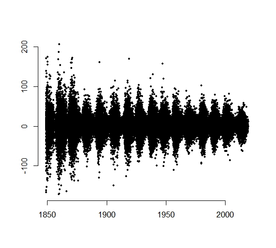
Source: WDC-SILSO, Royal Observatory of Belgium, Brussels, http://www.sidc.be/silso/datafiles, accessed on April 3, 2019. from 1848/12/23 to 2019/03/31 having daily observations. Time series of sunspots are often analyzed using fBm models, see, for instance, Shaikh et al. 2008. Estimator (3) and the second-order increments ratio estimator from Bardet and
Surgailis 2011 applied to all data both yield . However, , such that we clearly reject the hypothesis that is constant. A classical R/S estimate from the increments yields a different value of ca. 0.32 for . This method is often used in the applied literature. We do not rely on this R/S method, however, since Bardet 2018 notes that “a convincing asymptotic study of such an estimator” does not exist, and Taqqu
et al. 1995 have demonstrated that the obtained estimates are in general not accurate. Sunspots have a periodic behavior with at least one cycle of about 11 years, compare Figure 3. Especially for non-stationary time series, we obtained inaccurate R/S Hurst exponent estimates also in simulation experiments.
The right-plot of Figure 3 shows 21 point estimates for the Hurst exponent on time blocks with 3,000 days. Since more than 10,000 daily increments and around 2,000 second-order increments are zero, we need to adjust the increments ratio estimator and we see some relevant differences between both estimators. Nevertheless, the empirical findings allow to conclude that a multifractional Brownian motion model is better suited and that the Hurst exponent is not constant and has larger values in a period after 1950 than before. Looking at sub-samples of the time series, we find that for 3-years block length the test does not reject the hypothesis of a constant Hurst exponent in these blocks at 10%-level in 7 of the 63 blocks with a minimum value of . For 1-year block length it is not rejected for 81 from 170 years. This indicates that within smaller time intervals fBm may be used as a suitable model.


References
- Bardet (2018) Bardet, J.-M. (2018). Theoretical and numerical comparisons of the parameter estimator of the fractional Brownian motion. In Mathematical structures and applications, STEAM-H: Sci. Technol. Eng. Agric. Math. Health, pp. 153–173. Springer, Cham.
- Bardet and Surgailis (2011) Bardet, J.-M. and D. Surgailis (2011). Measuring the roughness of random paths by increment ratios. Bernoulli 17(2), 749–780.
- Bégyn (2007) Bégyn, A. (2007). Functional limit theorems for generalized quadratic variations of gaussian processes. Stochastic Process. Appl., 117(12), 1848 – 1869.
- Betken (2017) Betken, A. (2017). Change point estimation based on wilcoxon tests in the presence of long-range dependence. Electron. J. Statist. 11(2), 3633–3672.
- Bibinger and Madensoy (2019) Bibinger, M. and M. Madensoy (2019). Change-point inference on volatility in noisy Itô semimartingales. Stochastic Process. Appl., 129(12), 4878 – 4925.
- Breuer and Major (1983) Breuer, P. and P. Major (1983). Central limit theorems for nonlinear functionals of Gaussian fields. J. Multivariate Anal. 13(3), 425–441.
- Brouste and Fukasawa (2018) Brouste, A. and M. Fukasawa (2018). Local asymptotic normality property for fractional Gaussian noise under high-frequency observations. Ann. Statist. 46(5), 2045–2061.
- Coeurjolly (2000) Coeurjolly, J.-F. (2000). Simulation and identification of the fractional Brownian motion: a bibliographical and comparative study. J. Stat. Softw. 50(7), 1–53.
- Coeurjolly (2001) Coeurjolly, J.-F. (2001). Estimating the parameters of a fractional Brownian motion by discrete variations of its sample paths. Stat. Inference Stoch. Process. 4(2), 199–227.
- Coeurjolly and Istas (2001) Coeurjolly, J.-F. and J. Istas (2001). Cramér-Rao bounds for fractional Brownian motions. Statist. Probab. Lett. 53(4), 435–447.
- Ingster and Suslina (2003) Ingster, Y. I. and I. A. Suslina (2003). Nonparametric goodness-of-fit testing under Gaussian models, Volume 169 of Lecture Notes in Statistics. Springer-Verlag, New York.
- Jacod and Protter (2012) Jacod, J. and P. Protter (2012). Discretization of processes. Springer.
- Lavancier et al. (2013) Lavancier, F., R. Leipus, A. Philippe, and D. Surgailis (2013). Detection of nonconstant long memory parameter. Econometric Theory 29(5), 1009–1056.
- Nourdin (2012) Nourdin, I. (2012). Selected aspects of fractional Brownian motion. Milano: Springer.
- Nourdin and Nualart (2019) Nourdin, I. and D. Nualart (2019). The functional breuer–major theorem. Probab. Theory Related Fields, forthcoming.
- Nourdin et al. (2010) Nourdin, I., D. Nualart, and C. A. Tudor (2010). Central and non-central limit theorems for weighted power variations of fractional Brownian motion. Ann. Inst. Henri Poincaré Probab. Stat. 46(4), 1055–1079.
- Phillips (1987) Phillips, P. C. B. (1987). Time series regression with a unit root. Econometrica 55(2), 277–301.
- Shaikh et al. (2008) Shaikh, Y. H., A. R. Khan, M. I. Iqbal, S. H. Behere, and S. P. Bagare (2008). Sunspots data analysis using time series. Fractals 16(03), 259–265.
- Taqqu et al. (1995) Taqqu, M. S., V. Teverovsky, and W. Willinger (1995). Estimators for long-range dependence: An empirical study. Fractals 03(04), 785–798.