On the Adaptivity of Stochastic Gradient-Based Optimization

The application of gradient-based optimization methodology to statistical machine learning has been a major success story, in practice and in theory. Indeed, there is an increasingly detailed theory available for gradient-based algorithms that helps to explain their practical success. There remains, however, a significant gap between theory and practice, in that the designer of machine learning algorithms is required to make numerous choices that depend on parameters that are unlikely to be known in a real-world machine-learning setting. For example, existing theory asserts that different algorithms are preferred if a problem is strongly convex or merely convex, if the target accuracy is high or low, if the signal-to-noise is high or low and if data are independent or correlated. This poses a serious challenge to builders of machine-learning software, and to users of that software. Indeed, a distinctive aspect of machine-learning problems, especially large-scale problems, is that the user of an algorithm can be expected to know little or nothing about quantitative structural properties of the functions being optimized. It is hoped that the data and the data analysis will inform such properties, not the other way around.

To take a classical example, the stochastic gradient descent (SGD) algorithm takes different forms for strongly convex objectives and non-strongly convex objectives. In the former case, letting $\mu$ denote the strong-convexity parameter, if the stepsize is set as $O(1/\mu t)$ then SGD exhibits a convergence rate of $O(1/\mu\epsilon)$, where $\epsilon$ is the target accuracy [39]. In the latter case setting the stepsize to $O(1/\sqrt{t})$ yields a rate of $O(1/\epsilon^{2})$ [38]. Using the former scheme for non-strongly convex objectives can significantly deteriorate the convergence [38]. It is sometimes suggested that one can insure strong convexity by simply adding a quadratic regularizer to the objective, using the coefficient of the regularizer as a conservative estimate of the strong-convexity parameter. But this produces a significantly faster rate only if $\mu\gg\epsilon$, a regime that is unrealistic in many machine-learning applications, where $\epsilon$ is relatively large. Setting $\mu$ to such a large value would have a major effect on the statistical properties of the optimizer.

Similar comments apply to presumptions of knowledge of Lipschitz parameters, mini-batch sizes, variance-reduction tuning parameters, etc. Current practice often involves heuristics in setting these tuning parameters, but the use of these heuristics can change the algorithm and the optimality guarantees may disappear.

Our goal, therefore, should be that our algorithms are adaptive, in the sense that they perform as well as an algorithm that is assumed to know the “correct” choice of tuning parameters, even if they do not know those parameters. In particular, in the convex setting, we wish to derive an algorithm that does not involve $\mu$ in its implementation but whose convergence rate would be better for larger $\mu$ while still reasonable for smaller $\mu$, including the non-strongly convex case where $\mu=0$.

Such adaptivity has been studied implicitly in the classic literature. [50] and [45] and [46] showed that the average iterate of SGD with stepsize $O(t^{-\alpha})$ for $\alpha\in(1/2,1)$ satisfies a central limit theorem with information-theoretically optimal asymptotic variance. This implies adaptivity because the performance adapts to the underlying parameters of the problem, including the modulus of strong convexity, even though the algorithm does not require knowledge of them. The analysis by [46] is, however, asymptotic and relies on the smoothness of Hessian. Under similar assumptions on the Hessian, [37] provided a non-asymptotic analysis establishing adaptivity of SGD with Polyak-Ruppert averaging. Further contributions to this line of work include [7, 16, 11], who prove the adaptivity of certain versions of SGD with refined rates for self-concordant objectives, including least-square regression and logistic regression.

This line of work relies on conditions on higher-order derivatives which are not required in the modern literature on stochastic gradient methods. In fact, under fairly standard assumptions for first-order methods, [37] provided a non-asymptotic analysis for SGD with stepsize $O(t^{-\alpha})$ without averaging and showed that this algorithm exhibits adaptivity to strong convexity while having reasonable guarantee for non-strongly convex objectives. Specifically, if $\alpha=2/3$, their results show that the rate to achieve an $\epsilon$-accurate solution for the expected function value is $\tilde{O}\big(\min\big\{1/\mu^{3}+1/\mu\epsilon^{2},$ $1/\epsilon^{3}\big\}\big)$, where $\tilde{O}$ hides logarithmic factors. This result was taken further by studying alternative stepsize schemes; in particular, [60] proposed a variant of projected SGD with stagewise diminishing stepsizes and diameters. Unlike the aforementioned work, the adaptivity in this case is weaker because it requires knowledge of the strong convexity parameter, as well as the initial suboptimality, in the complexity analysis (in particular, they require a sufficiently large initial diameter). A weaker form of adaptivity, to smoothness but not to strong convexity, was established by [32] when the polynomial decaying stepsize is replaced by an AdaGrad-type stepsize [13], assuming a bounded domain and bounded stochastic gradients. Finally, [9] presented a restarting variant of AdaGrad with provable adaptivity to strong convexity given an initial overestimate of the strong convexity parameter.

Further progress has been made by focusing on a setting that is particularly relevant to machine learning—that of finite-sum optimization. The objective function in this setting takes the following form:

where $\mathcal{X}$ is the parameter space, $n$ is the number of data points, the functions $f_{i}(x)$ are data-point-specific loss functions and $\psi(x)$ is the regularization term. We assume that each $f_{i}(x)$ is differentiably convex and $\psi(x)$ is convex but can be non-differentiable. The introduction of the parameter $n$ into the optimization problem has two important implications. First, it implies that the number of operations to obtain a full gradient is $O(n)$, which is generally impractical in modern machine-learning applications, where the value of $n$ can be in the tens to hundreds of millions. This fact motivates us to make use of stochastic estimates of gradients. Such randomness introduces additional variance that interacts with the variability of the data, and tuning parameters are often introduced to control this variance.

Second, the finite-sum formulation highlights the need for adaptivity to the target accuracy $\epsilon$, where that accuracy is related to the number of data points $n$ for statistical reasons. Unfortunately, different algorithms perform better in high-accuracy versus low-accuracy regimes, and the choice of regime is generally not clear to a user of machine-learning algorithms, given that target accuracy varies not only as a function of $n$, but also as a function of other parameters, such as the signal-to-noise ratio, that the user is not likely to know. Ideally, therefore, optimization algorithms should be adaptive to target accuracy, performing well in either regime.

Deterministic gradient-descent-based methods can be made adaptive to strong convexity and smoothness simultaneously by exploiting the Polyak stepsize [18]. However, computation of a full gradient is expensive, rendering the method undesirable for finite-sum optimization. A recent line of research has shown that algorithms with lower complexity can be designed in the finite-sum setting with some adaptivity, generally via careful control of the variance. The stochastic average gradient (SAG) method opened this line of research, establishing a complexity of $\tilde{O}\left(\min\{n/\epsilon,n+L/\mu\}\right)$ [49]. Importantly, this result shows that SAG is adaptive to strong convexity. To achieve such adaptivity, however, SAG requires two sequences of iterates, the average iterate and the last iterate. [10] propose a single-sequence variant of SAG that is also adaptive to strong convexity, yet under stronger assumption that each $f_{i}$ is strongly convex. Both methods suffer, however, from a prohibitive storage cost of $O(nd)$, where $d$ is the dimension of $\mathcal{X}$. Further developments in this vein include the stochastic variance reduced gradient (SVRG) method [22] and the stochastic dual coordinate ascent (SDCA) method [22]; they achieve the same computational complexity as SAG while reducing the storage cost to $O(d)$. They are not, however, adaptive to strong convexity.

[30] presented a randomized variant of SVRG that achieves the same convergence rate and adaptivity as SAG but with the same storage cost as SVRG. However, as is the case with SAG, the complexity of $O(n/\epsilon)$ for the non-strongly convex case is much larger than the oracle lower bound of $O(n+\sqrt{n/\epsilon})$ [58]. [41] propose another variance-reduction method that is provably adaptive to strong convexity, though the result is proved for the expected gradient norm and is thus weaker than [30]. [59] develop another variant of SVRG which adapts to a more general condition, called a “Hölderian error bound,” with strong convexity being a special case. In contrast to [30], they required an initial conservative estimate of the strong convexity parameter. Under an extra strong assumption of gradient interpolation—that all individual loss functions have vanishing gradients at the optimum—[56] developed an algorithm that achieves adaptivity to the smoothness parameter and to the modulus of strong convexity simultaneously. On the other hand, recent work of [28] that came after our work presents an algorithm that achieves certain adaptivity to the target accuracy. However, they need to know the modulus of strong convexity and the adaptivity is only obtained in the high-accuracy regime because it requires full gradient computations periodically. Finally, while our focus is convex optimization, we note that adaptivity has also been studied for nonconvex finite-sum optimization (e.g., [31, 43]).

In this article we present an algorithm, the stochastically controlled stochastic gradient (SCSG) algorithm, that exhibits adaptivity both to strong convexity and to target accuracy. SCSG is a nested procedure that is similar to the SVRG algorithm. Crucially, it does not require the computation of a full gradient in the outer loop as performed by SVRG, but makes use of stochastic estimates of gradients in both the outer loop and the inner loop. Moreover, it makes essential use of a randomization technique (“geometrization”) that allows terms to telescope across the outer loop and the inner loops; such telescoping does not happen in SVRG, a fact which leads to the loss of adaptivity for SVRG.

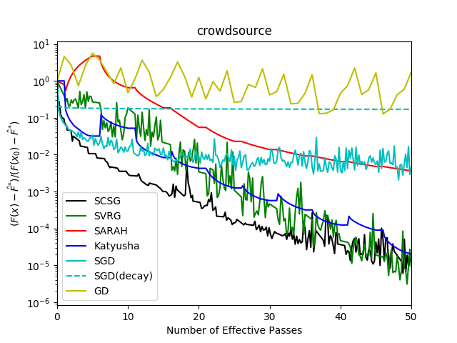
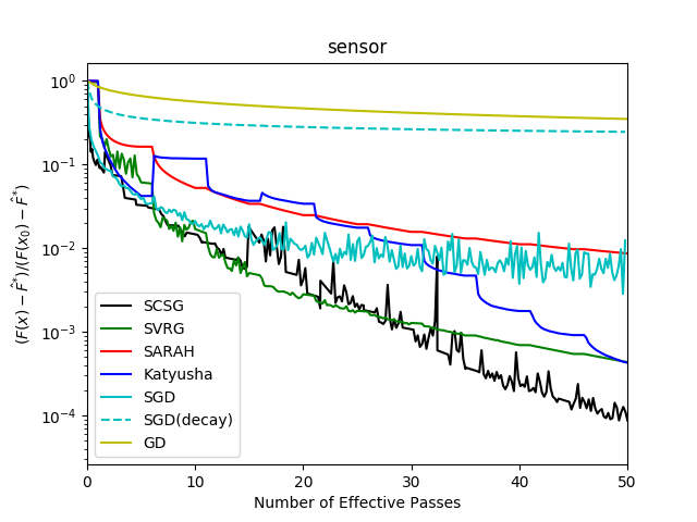
The rest of the article is organized as follows: Section 2 introduces notation, assumptions and definitions. In Section 3 and Section 4, we focus on the relatively simple setting of unregularized problems and Euclidean geometry, introducing the key ideas of geometrization and adaptive batching. We provide key proofs in Section 4 and leave non-essential proofs into Appendix A in the Supplementary Material. We extend these results to regularized problems and to non-Euclidean geometry in Section 5. The extension relaxes standard assumptions for analyzing mirror descent methods and may be of independent interest. All proofs for the general case are relegated into Appendix B and some miscellaneous results are presented in Appendix C in Supplementary Material. Finally, the desirable empirical performance of SCSG is demonstrated in Appendix D.

We write $a\wedge b$ (resp. $a\vee b$) for $\min\{a,b\}$ (resp. $\max\{a,b\}$), and $(a)_{*}^{\xi}$ (or $[a]_{*}^{\xi}$) for $\max\{a,1\}^{\xi}$ throughout the paper. The symbol $\mathbb{E}$ denotes the expectation of a random element and $\mathbb{E}_{X}$ denotes an expectation over the randomness of $X$ while conditioning on all other random elements. We adopt Landau’s notation ($O(\cdot),o(\cdot)$), and we occasionally use $\tilde{O}(\cdot)$ to hide logarithmic factors. We define computational cost by making use of the IFO framework of [1, 47], where we assume that sampling an index $i$ and computing the pair $(f_{i}(x),\nabla f_{i}(x))$ incurs a unit of cost. For notational convenience, given a subset $\mathcal{I}\subset\{1,\ldots,n\}$, we denote by $\nabla f_{\mathcal{I}}(x)$ the batch gradient:

By definition, computing $\nabla f_{\mathcal{I}}(x)$ incurs $|\mathcal{I}|$ units of cost.

In this section and the following two sections we focus on unregularized problems and Euclidean geometry, turning to regularized problems and non-Euclidean geometry in Section 5. Specifically, we consider the case $\mathcal{X}=\mathbb{R}^{d}$, $\psi\equiv 0$ and make the following assumptions that target the finite-sum optimization problem:

1. A1

   $f_{i}$ is convex with $L$-Lipschitz gradient

   $$f_{i}(x)-f_{i}(y)-\langle\nabla f_{i}(y),x-y\rangle\leq\frac{L}{2}\|x-y\|_{2}^{2},\quad\forall i=1,\ldots,n,$$

   for some $L<\infty$;

2. A2

   $F=f$ is strongly convex at $x^{*}$ with

   $$f(x)-f(x^{*})\geq\frac{\mu}{2}\|x-x^{*}\|_{2}^{2},$$

   for some $\mu\geq 0$.

Note that assumption A2 always holds with $\mu=0$, corresponding to the non-strongly convex case. Note also that with the exception of [49], this assumption is weaker than most of the the literature on smooth finite-sum optimization, where strong convexity of $f$ is required at every point.

Our analysis will make use of the following key quantity [30]:

where $x^{*}$ denotes the optimum of $f$. If multiple optima exist we take one that minimizes $\mathcal{H}(f)$. We use $\mathcal{H}(f)$, an average squared norm at the optimum, in place of the uniform upper bound on the gradient that is often assumed in other work. The latter is not realistic for many practical problems in machine learning, including least squares, where the gradient is unbounded. On the other hand, it is noteworthy that $\mathcal{H}(f)$ only depends on the optimum. For instance, $\mathcal{H}(f)=0$ if all gradients vanish at the optimum, as studied for over-parametrized models (e.g., [36, 55, 56]). As will be shown later, the complexity of our algorithm only depends on $\mathcal{H}(f)$ so it can be applied to study the case with data interpolation. We will write $\mathcal{H}(f)$ as $\mathcal{H}$ when no confusion can arise.

We let $\tilde{x}_{0}$ denote the initial value (possibly random) and define the following measures of complexity:

Recall that a geometric random variable, $N\sim\mathrm{Geom}(\gamma)$, is a discrete random variable with probability mass function $P(N=k)=(1-\gamma)\gamma^{k},\mbox{for}\ k=0,1,\ldots$, and expectation:

Geometric random variables will play a key role in the design and analysis of our algorithm.

Finally, we introduce two fundamental definitions that serve to clarify desirable properties of optimization algorithms. We refer to the first property as $\epsilon$-independence. {definition*} An algorithm is $\mathbf{\epsilon}$-independent if it guarantees convergence at all target accuracies $\epsilon$.

$\epsilon$-independence is a crucial property in practice because a target accuracy is usually not exactly known apriori. An $\epsilon$-independent algorithm satisfies the “one-pass-for-all” property where the theoretical complexity analysis applies to the whole path of the iterates. In contrast, an $\epsilon$-dependent algorithm only has a theoretical guarantee for a particular $\epsilon$, whose value is often unknown in practice. To illustrate we consider SGD, where the iterate is updated by $x_{k+1}=x_{k}-\eta_{k}\nabla f_{i_{k}}(x_{k})$ and where $i_{k}$ is a uniform index from $\{1,\ldots,n\}$. There are two popular schemes for theoretical analysis: (1) $\eta_{k}=O(1/\sqrt{k})$ or (2) $\eta_{k}\equiv 1/\sqrt{T}$ and the iterates are updated for $O(T)$ steps where $T=O(1/\epsilon^{2})$. Although both versions have theoretical complexity $\tilde{O}\left(\epsilon^{-2}\right)$, only the former is $\epsilon$-independent.

The second important property is referred to as almost universality. {definition*} An algorithm is almost universal if it only requires the knowledge of the smoothness parameters $L$.

The term almost universality is motivated by the notion of universality introduced by [40] which does not require the knowledge of $L$ or other parameters such as the variance of the stochastic gradients. Returning to the previous example, both versions of SGD are universal. It is noteworthy that universal gradient methods are usually either $\epsilon$-dependent (e.g. [40]) or require imposing other assumptions such as uniformly bounded $\nabla f_{i}$ (e.g. [38]). The SCSG algorithm developed in this paper is both $\epsilon$-independent and almost universal. This category also includes SGD for general convex functions [38], SAG [49], SAGA [10], SVRG++ [5], Katyusha for non-strongly convex functions [3], and AMSVRG [42]. In contrast, algorithms such as SGD for strongly convex functions [38], SVRG [22], SDCA [51], APCG [35], Katyusha for strongly convex functions [3] and adaptive SVRG [59] are $\epsilon$-independent but not almost universal because they need full or partial knowledge of $\mu$. Furthermore, algorithms such as Catalyst [34] and AdaptReg [4] even depend on unknown quantities such as $F(x_{0})-F(x^{*})$ or the variance of the $\nabla f_{i}$. In comparing algorithms we believe that clarity on these distinctions is critical, in addition to comparison of convergence rates.

In this section we present SCSG, a computationally efficient framework for variance reduction in stochastic gradient descent algorithms. SCSG builds on the SVRG algorithm of [22], incorporating several essential modifications that yield not only computational efficiency but also adaptivity. Recall that SVRG is a nested procedure that computes a full gradient in each outer loop and uses that gradient as a baseline to reduce the variance of the stochastic gradients that are computed in an inner loop. The need to compute a full gradient, at a cost of $n$ operations, unfortunately makes the SVRG procedure impractical for large-scale applications. SCSG seeks to remove this bottleneck by replacing the full gradient with an approximate, stochastic gradient, one that is based on a batch size that is significantly smaller than $n$ but larger than the size used for the stochastic gradients in the inner loop. By carefully weighing the contributions to the bias and variance of these sampling-based estimates, SCSG achieves a small iteration complexity while also keeping the per-iteration complexity feasibly small.

Further support for the SCSG framework comes from the comparison with SVRG in the setting of strongly convex objectives. In this setting, SVRG relies heavily on a presumption of knowledge of the strong convexity parameter $\mu$. In particular, to achieve a complexity of $O((n+\kappa)\log(1/\epsilon))$, the number of stochastic gradients queried in the inner loop of SVRG needs to scale as $\kappa$. By contrast, the SCSG framework achieves the same complexity without knowledge of $\mu$. This is achieved by setting the number of inner-loop stochastic gradients to be a geometric random variable. As we discuss below, the usage of a geometric random variable—a technique that we refer to as “geometrization”—is crucial in the design and analysis of SCSG. We believe that it is a key theoretical tool for achieving adaptivity to strong convexity.

The original version of SCSG was $\epsilon$-dependent and not almost universal, because it required knowledge of the parameter $\mathcal{H}$ [30]. Moreover the algorithm had a sub-optimal rate in the high-accuracy regime. In further development of the SCSG framework, in the context of nonconvex optimization [31], we found that $\epsilon$-independence and almost universality could be achieved by employing an increasing sequence of batch sizes.

In the remainder of this section, we bring these ideas together and present the general form of the SCSG algorithm, incorporating adaptive batching, geometrization and mini-batches in the inner loop. The resulting algorithm is adaptive, $\epsilon$-independent and almost universal. Roughly speaking, the adaptive batching enables the adaptivity to target accuracy and the geometrization enables the adaptivity to strong convexity. The pseudocode for SCSG is shown in Algorithm 1. Guidelines for practical choice for the parameters is provided in Remark 5 in Section 4.2. As can be seen, the algorithm is superficially complex, but, as in the case of line-search and trust-region methods that augment simple gradient-based methods in deterministic optimization, the relative lack of dependence on hyperparameters makes the algorithm robust and relatively easy to deploy.

Note that in Algorithm 1, and throughout the paper, we use $\tilde{x}_{j}$ to denote the iterate in the $j$th outer loop and $x_{k}^{(j)}$ to denote the iterate in the $k$th step of the $j$th inner loop.

To measure the computational complexity of SCSG, let $T(\epsilon)$ denote the first time step at which $\tilde{x}_{T}$ is an $\epsilon$-approximate solution, as well as all following iterates $\tilde{x}_{T+1},\tilde{x}_{T+2},\ldots$:

This criterion is more stringent than those considered in some other work which neglects the performance of $\tilde{x}_{T}$ for $T>T(\epsilon)$. The computational cost incurred for computing $\tilde{x}_{T}$ is

Noting that $C_{\mathrm{comp}}(\epsilon)$ is random, we consider the average complexity obtained by taking the expectation of $C_{\mathrm{comp}}(\epsilon)$. Since $N_{j}\sim\mathrm{Geom}(\frac{m_{j}}{m_{j}+b_{j}})$, we have:

References

• [1] A. Agarwal and L. Bottou, A lower bound for the optimization of finite sums, ArXiv e-prints abs/1410.0723, (2014).
• [2] A. Agarwal, M. J. Wainwright, P. L. Bartlett, and P. K. Ravikumar, Information-theoretic lower bounds on the oracle complexity of convex optimization, in Advances in Neural Information Processing Systems, 2009, pp. 1–9.
• [3] Z. Allen-Zhu, Katyusha: The first direct acceleration of stochastic gradient methods, in Proceedings of the 49th Annual ACM SIGACT Symposium on Theory of Computing, ACM, 2017, pp. 1200–1205.
• [4] Z. Allen-Zhu and E. Hazan, Optimal black-box reductions between optimization objectives, in Advances in Neural Information Processing Systems, 2016, pp. 1614–1622.
• [5] Z. Allen-Zhu and Y. Yuan, Improved SVRG for non-strongly-convex or sum-of-non-convex objectives, in International conference on machine learning, 2016, pp. 1080–1089.
• [6] Y. Arjevani, Limitations on variance-reduction and acceleration schemes for finite sum optimization, arXiv preprint arXiv:1706.01686, (2017).
• [7] F. Bach and E. Moulines, Non-strongly-convex smooth stochastic approximation with convergence rate o (1/n), in Advances in neural information processing systems, 2013, pp. 773–781.
• [8] A. Beck and M. Teboulle, Mirror descent and nonlinear projected subgradient methods for convex optimization, Operations Research Letters, 31 (2003), pp. 167–175.
• [9] Z. Chen, Y. Xu, E. Chen, and T. Yang, SADAGRAD: Strongly adaptive stochastic gradient methods, in International Conference on Machine Learning, 2018, pp. 912–920.
• [10] A. Defazio, F. Bach, and S. Lacoste-Julien, SAGA: A fast incremental gradient method with support for non-strongly convex composite objectives, in Advances in Neural Information Processing Systems, 2014, pp. 1646–1654.
• [11] A. Dieuleveut, N. Flammarion, and F. Bach, Harder, better, faster, stronger convergence rates for least-squares regression, Journal of Machine Learning Research, 18 (2017), pp. 3520–3570.
• [12] D. Dua and C. Graff, UCI machine learning repository, 2017, http://archive.ics.uci.edu/ml.
• [13] J. Duchi, E. Hazan, and Y. Singer, Adaptive subgradient methods for online learning and stochastic optimization, Journal of Machine Learning Research, 12 (2011), pp. 2121–2159.
• [14] J. C. Duchi, S. Shalev-Shwartz, Y. Singer, and A. Tewari, Composite objective mirror descent., in Conference on Learning Theory, 2010, pp. 14–26.
• [15] L. Dümbgen, S. A. Van De Geer, M. C. Veraar, and J. A. Wellner, Nemirovski’s inequalities revisited, The American Mathematical Monthly, 117 (2010), pp. 138–160.
• [16] N. Flammarion and F. Bach, From averaging to acceleration, there is only a step-size, in Conference on Learning Theory, 2015, pp. 658–695.
• [17] O. Hanner, On the uniform convexity of Lp{L}_{p} and ℓp\ell_{p}, Arkiv för Matematik, 3 (1956), pp. 239–244.
• [18] E. Hazan and S. Kakade, Revisiting the polyak step size, arXiv preprint arXiv:1905.00313, (2019).
• [19] E. Hazan and S. Kale, An optimal algorithm for stochastic strongly-convex optimization, arXiv preprint arXiv:1006.2425, (2010).
• [20] W. Hoeffding, Probability inequalities for sums of bounded random variables, Journal of the American statistical association, 58 (1963), pp. 13–30.
• [21] B. A. Johnson and K. Iizuka, Integrating openstreetmap crowdsourced data and landsat time-series imagery for rapid land use/land cover (lulc) mapping: Case study of the laguna de bay area of the philippines, Applied Geography, 67 (2016), pp. 140–149.
• [22] R. Johnson and T. Zhang, Accelerating stochastic gradient descent using predictive variance reduction, in Advances in Neural Information Processing Systems, 2013, pp. 315–323.
• [23] A. Juditsky, A. Nemirovski, and C. Tauvel, Solving variational inequalities with stochastic mirror-prox algorithm, Stochastic Systems, 1 (2011), pp. 17–58.
• [24] A. Juditsky and Y. Nesterov, Deterministic and stochastic primal-dual subgradient algorithms for uniformly convex minimization, Stochastic Systems, 4 (2014), pp. 44–80.
• [25] R. Kohavi, Scaling up the accuracy of naive-bayes classifiers: A decision-tree hybrid., in Kdd, vol. 96, Citeseer, 1996, pp. 202–207.
• [26] G. Lan, An optimal method for stochastic composite optimization, Mathematical Programming, 133 (2012), pp. 365–397.
• [27] G. Lan, An optimal randomized incremental gradient method, ArXiv e-prints abs/1507.02000, (2015).
• [28] G. Lan, Z. Li, and Y. Zhou, A unified variance-reduced accelerated gradient method for convex optimization, arXiv preprint arXiv:1905.12412, (2019).
• [29] Y. LeCun, L. Bottou, Y. Bengio, and P. Haffner, Gradient-based learning applied to document recognition, Proceedings of the IEEE, 86 (1998), pp. 2278–2324.
• [30] L. Lei and M. I. Jordan, Less than a single pass: Stochastically controlled stochastic gradient method, arXiv preprint arXiv:1609.03261, (2016).
• [31] L. Lei, C. Ju, J. Chen, and M. I. Jordan, Non-convex finite-sum optimization via scsg methods, in Advances in Neural Information Processing Systems, 2017, pp. 2345–2355.
• [32] Y. K. Levy, A. Yurtsever, and V. Cevher, Online adaptive methods, universality and acceleration, in Advances in Neural Information Processing Systems, 2018, pp. 6500–6509.
• [33] M. Li, T. Zhang, Y. Chen, and A. J. Smola, Efficient mini-batch training for stochastic optimization, in Proceedings of the 20th ACM SIGKDD international conference on Knowledge discovery and data mining, ACM, 2014, pp. 661–670.
• [34] H. Lin, J. Mairal, and Z. Harchaoui, A universal catalyst for first-order optimization, in Advances in Neural Information Processing Systems, 2015, pp. 3384–3392.
• [35] Q. Lin, Z. Lu, and L. Xiao, An accelerated proximal coordinate gradient method, in Advances in Neural Information Processing Systems, 2014, pp. 3059–3067.
• [36] S. Ma, R. Bassily, and M. Belkin, The power of interpolation: Understanding the effectiveness of SGD in modern over-parametrized learning, arXiv preprint arXiv:1712.06559, (2017).
• [37] E. Moulines and F. R. Bach, Non-asymptotic analysis of stochastic approximation algorithms for machine learning, in Advances in Neural Information Processing Systems, 2011, pp. 451–459.
• [38] A. Nemirovski, A. Juditsky, G. Lan, and A. Shapiro, Robust stochastic approximation approach to stochastic programming, SIAM Journal on Optimization, 19 (2009), pp. 1574–1609.
• [39] Y. Nesterov, Introductory Lectures on Convex Optimization: A Basic Course, Kluwer Academic Publishers, Massachusetts, 2004.
• [40] Y. Nesterov, Universal gradient methods for convex optimization problems, Mathematical Programming, 152 (2015), pp. 381–404.
• [41] L. M. Nguyen, M. van Dijk, D. T. Phan, P. H. Nguyen, T.-W. Weng, and J. R. Kalagnanam, Finite-sum smooth optimization with SARAH, def, 1 (2019), p. 1.
• [42] A. Nitanda, Accelerated stochastic gradient descent for minimizing finite sums, in Artificial Intelligence and Statistics, 2016, pp. 195–203.
• [43] C. Paquette, H. Lin, D. Drusvyatskiy, J. Mairal, and Z. Harchaoui, Catalyst acceleration for gradient-based non-convex optimization, arXiv preprint arXiv:1703.10993, (2017).
• [44] G. Pisier, Martingales with values in uniformly convex spaces, Israel Journal of Mathematics, 20 (1975), pp. 326–350.
• [45] B. T. Polyak, New stochastic approximation type procedures, Automat. i Telemekh, 7 (1990), p. 2.
• [46] B. T. Polyak and A. B. Juditsky, Acceleration of stochastic approximation by averaging, SIAM Journal on Control and Optimization, 30 (1992), pp. 838–855.
• [47] S. J. Reddi, A. Hefny, S. Sra, B. Poczos, and A. Smola, Stochastic variance reduction for nonconvex optimization, arXiv preprint arXiv:1603.06160, (2016).
• [48] I. Rodriguez-Lujan, J. Fonollosa, A. Vergara, M. Homer, and R. Huerta, On the calibration of sensor arrays for pattern recognition using the minimal number of experiments, Chemometrics and Intelligent Laboratory Systems, 130 (2014), pp. 123–134.
• [49] N. L. Roux, M. Schmidt, and F. Bach, A stochastic gradient method with an exponential convergence rate for finite training sets, in Advances in Neural Information Processing Systems, 2012, pp. 2663–2671.
• [50] D. Ruppert, Efficient estimators from a slowly convergent Robbins-Monro procedure, School of Oper. Res. and Ind. Eng., Cornell Univ., Ithaca, NY, Tech. Rep, 781 (1988).
• [51] S. Shalev-Shwartz and T. Zhang, Proximal stochastic dual coordinate ascent, ArXiv e-prints abs/1211.2717, (2012).
• [52] S. Shalev-Shwartz and T. Zhang, Accelerated proximal stochastic dual coordinate ascent for regularized loss minimization., in International Conference on Machine Learning, 2014, pp. 64–72.
• [53] O. Shamir, Making gradient descent optimal for strongly convex stochastic optimization, CoRR abs/1109.5647, (2011).
• [54] N. Srebro, K. Sridharan, and A. Tewari, On the universality of online mirror descent, in Advances in neural information processing systems, 2011, pp. 2645–2653.
• [55] S. Vaswani, F. Bach, and M. Schmidt, Fast and faster convergence of SGD for over-parameterized models and an accelerated perceptron, arXiv preprint arXiv:1810.07288, (2018).
• [56] S. Vaswani, A. Mishkin, I. Laradji, M. Schmidt, G. Gidel, and S. Lacoste-Julien, Painless stochastic gradient: Interpolation, line-search, and convergence rates, arXiv preprint arXiv:1905.09997, (2019).
• [57] A. Vergara, S. Vembu, T. Ayhan, M. A. Ryan, M. L. Homer, and R. Huerta, Chemical gas sensor drift compensation using classifier ensembles, Sensors and Actuators B: Chemical, 166 (2012), pp. 320–329.
• [58] B. Woodworth and N. Srebro, Tight complexity bounds for optimizing composite objectives, ArXiv e-prints abs/1605.08003, (2016).
• [59] Y. Xu, Q. Lin, and T. Yang, Adaptive SVRG methods under error bound conditions with unknown growth parameter, in Advances in Neural Information Processing Systems, 2017, pp. 3279–3289.
• [60] Y. Xu, Q. Lin, and T. Yang, Accelerate stochastic subgradient method by leveraging local growth condition, Analysis and Applications, 17 (2019), pp. 773–818.
• [61] I.-C. Yeh and C.-h. Lien, The comparisons of data mining techniques for the predictive accuracy of probability of default of credit card clients, Expert Systems with Applications, 36 (2009), pp. 2473–2480.
Supplementary Material
Appendix A Technical Proofs in Section 4
Proof of Lemma 8.
Using the fact that 𝔼​‖Z‖22=𝔼​‖Z−𝔼​Z‖22+‖𝔼​Z‖22\mathbb{E}\|Z\|_{2}^{2}=\mathbb{E}\|Z-\mathbb{E}Z\|_{2}^{2}+\|\mathbb{E}Z\|_{2}^{2} (for any random vector ZZ), we have
𝔼ℐ~k(j)​‖νk(j)‖22=𝔼ℐ~k(j)​‖νk(j)−𝔼ℐ~k(j)​νk(j)‖22+‖𝔼ℐ~k(j)​νk(j)‖22\displaystyle\mathbb{E}_{\tilde{\mathcal{I}}^{(j)}_{k}}\|\nu^{(j)}_{k}\|_{2}^{2}=\mathbb{E}_{\tilde{\mathcal{I}}^{(j)}_{k}}\|\nu^{(j)}_{k}-\mathbb{E}_{\tilde{\mathcal{I}}^{(j)}_{k}}\nu^{(j)}_{k}\|_{2}^{2}+\|\mathbb{E}_{\tilde{\mathcal{I}}^{(j)}_{k}}\nu^{(j)}_{k}\|_{2}^{2}
=𝔼ℐ~k(j)​‖∇fℐ~k(j)​(xk(j))−∇fℐ~k(j)​(x0(j))−(∇f​(xk(j))−∇f​(x0(j)))‖22+‖∇f​(xk(j))+ej‖22\displaystyle=\mathbb{E}_{\tilde{\mathcal{I}}^{(j)}_{k}}\|\nabla f_{\tilde{\mathcal{I}}^{(j)}_{k}}(x^{(j)}_{k})-\nabla f_{\tilde{\mathcal{I}}^{(j)}_{k}}(x^{(j)}_{0})-(\nabla f(x^{(j)}_{k})-\nabla f(x^{(j)}_{0}))\|_{2}^{2}+\|\nabla f(x^{(j)}_{k})+e_{j}\|_{2}^{2}
≤1bj​n​(∑i=1n‖∇fi​(xk(j))−∇fi​(x0(j))‖22)+‖∇f​(xk(j))+ej‖22,\displaystyle\leq\frac{1}{b_{j}n}\left(\sum_{i=1}^{n}\|\nabla f_{i}(x^{(j)}_{k})-\nabla f_{i}(x^{(j)}_{0})\|_{2}^{2}\right)+\|\nabla f(x^{(j)}_{k})+e_{j}\|_{2}^{2},
where the last inequality is obtained from Lemma 30. By Lemma 29 with g=fi,x=x0(j),y=xk(j)g=f_{i},x=x^{(j)}_{0},y=x^{(j)}_{k},
‖∇fi​(xk(j))−∇fi​(x0(j))‖22\displaystyle\|\nabla f_{i}(x^{(j)}_{k})-\nabla f_{i}(x^{(j)}_{0})\|_{2}^{2} ≤2​L​(fi​(x0(j))−fi​(xk(j))+⟨∇fi​(xk(j)),xk(j)−x0(j)⟩).\displaystyle\leq 2L\left(f_{i}(x^{(j)}_{0})-f_{i}(x^{(j)}_{k})+\left\langle\nabla f_{i}(x^{(j)}_{k}),x^{(j)}_{k}-x^{(j)}_{0}\right\rangle\right).
The proof is completed by the fact that ‖a+b‖22=2​‖a‖22+2​‖b‖22−‖a−b‖22≤2​‖a‖22+2​‖b‖22\|a+b\|_{2}^{2}=2\|a\|_{2}^{2}+2\|b\|_{2}^{2}-\|a-b\|_{2}^{2}\leq 2\|a\|_{2}^{2}+2\|b\|_{2}^{2}.
Proof of Lemma 9.
Using the fact that ‖a+b‖22≤2​‖a‖22+2​‖b‖22\|a+b\|_{2}^{2}\leq 2\|a\|_{2}^{2}+2\|b\|_{2}^{2} and ∇f​(x∗)=0\nabla f(x^{*})=0, we have
𝔼​‖ej‖22≤2​𝔼​‖ej−∇fℐj​(x∗)‖22+2​𝔼​‖∇fℐj​(x∗)‖22\displaystyle\mathbb{E}\|e_{j}\|_{2}^{2}\leq 2\mathbb{E}\|e_{j}-\nabla f_{\mathcal{I}_{j}}(x^{*})\|_{2}^{2}+2\mathbb{E}\|\nabla f_{\mathcal{I}_{j}}(x^{*})\|_{2}^{2}
=2​𝔼​‖1Bj​∑i∈ℐj(∇fi​(x~j−1)−∇fi​(x∗))−(∇f​(x~j−1)−∇f​(x∗))‖22\displaystyle=2\mathbb{E}\left\|\frac{1}{B_{j}}\sum_{i\in\mathcal{I}_{j}}(\nabla f_{i}(\tilde{x}_{j-1})-\nabla f_{i}(x^{*}))-(\nabla f(\tilde{x}_{j-1})-\nabla f(x^{*}))\right\|_{2}^{2}
+2​𝔼​‖1Bj​∑i∈ℐj∇fi​(x∗)‖22.\displaystyle\hskip 14.22636pt+2\mathbb{E}\left\|\frac{1}{B_{j}}\sum_{i\in\mathcal{I}_{j}}\nabla f_{i}(x^{*})\right\|_{2}^{2}.
Then
𝔼​‖1Bj​∑i∈ℐj(∇fi​(x~j−1)−∇fi​(x∗))−(∇f​(x~j−1)−∇f​(x∗))‖22\displaystyle\mathbb{E}\left\|\frac{1}{B_{j}}\sum_{i\in\mathcal{I}_{j}}(\nabla f_{i}(\tilde{x}_{j-1})-\nabla f_{i}(x^{*}))-(\nabla f(\tilde{x}_{j-1})-\nabla f(x^{*}))\right\|_{2}^{2}
≤I⁡(Bj<n)Bj1n∑i=1n∥∇fi(x~j−1)−∇fi(x∗)∥22(Lemma 30)\displaystyle\leq\frac{I(B_{j}<n)}{B_{j}}\,\frac{1}{n}\sum_{i=1}^{n}\|\nabla f_{i}(\tilde{x}_{j-1})-\nabla f_{i}(x^{*})\|_{2}^{2}\quad(\mbox{Lemma \ref{lem:var_sampling}})
≤I⁡(Bj<n)Bj2​Ln∑i=1n(fi(x~j−1)−fi(x∗)−⟨∇fi(x∗),x~j−1−x∗⟩)(Lemma 29)\displaystyle\leq\frac{I(B_{j}<n)}{B_{j}}\,\frac{2L}{n}\sum_{i=1}^{n}\left(f_{i}(\tilde{x}_{j-1})-f_{i}(x^{*})-\left\langle\nabla f_{i}(x^{*}),\tilde{x}_{j-1}-x^{*}\right\rangle\right)\quad(\mbox{Lemma \ref{lem:cocoercive}})
=I⁡(Bj<n)Bj​ 2​L​(f⁡(x~j−1)−f⁡(x∗)−⟨∇f​(x∗),x~j−1−x∗⟩)\displaystyle=\frac{I(B_{j}<n)}{B_{j}}\,2L(f(\tilde{x}_{j-1})-f(x^{*})-\left\langle\nabla f(x^{*}),\tilde{x}_{j-1}-x^{*}\right\rangle)
=I⁡(Bj<n)Bj​ 2​L​(f⁡(x~j−1)−f⁡(x∗)).\displaystyle=\frac{I(B_{j}<n)}{B_{j}}\,2L(f(\tilde{x}_{j-1})-f(x^{*})).
On the other hand, by Lemma 30 again, we obtain that
𝔼​‖1Bj​∑i∈ℐj∇fi​(x∗)‖22≤ℋ​I​(Bj<n)Bj.\mathbb{E}\left\|\frac{1}{B_{j}}\sum_{i\in\mathcal{I}_{j}}\nabla f_{i}(x^{*})\right\|_{2}^{2}\leq\frac{\mathcal{H}\,I(B_{j}<n)}{B_{j}}.
Putting the pieces together we prove the result.
To prove the remaining two lemmas, we need an extra lemma that justifies the condition 𝔼​|DN|<∞\mathbb{E}|D_{N}|<\infty when applying geometrization (Lemma 1) in our proofs for different choices of {Dk}\{D_{k}\}. The proof is distracting and relegated to the end of this section.
Lemma 17.
Assume that ηj​L≤1/2\eta_{j}L\leq 1/2. Then for any jj,
𝔼​‖x~j−x∗‖22<∞,𝔼​‖νNj(j)‖22<∞,𝔼​|⟨ej,x~j−x~j−1⟩|<∞.\mathbb{E}\|\tilde{x}_{j}-x^{*}\|_{2}^{2}<\infty,\quad\mathbb{E}\|\nu^{(j)}_{N_{j}}\|_{2}^{2}<\infty,\quad\mathbb{E}|\left\langle e_{j},\tilde{x}_{j}-\tilde{x}_{j-1}\right\rangle|<\infty.
Proof of Lemma 10.
By definition,
𝔼ℐ~k(j)​‖xk+1(j)−u‖22=‖xk(j)−u‖22−2​ηj​𝔼ℐ~k(j)​⟨νk(j),xk(j)−u⟩+ηj2​𝔼ℐ~k(j)​‖νk(j)‖22\displaystyle\mathbb{E}_{\tilde{\mathcal{I}}^{(j)}_{k}}\|x^{(j)}_{k+1}-u\|_{2}^{2}=\|x^{(j)}_{k}-u\|_{2}^{2}-2\eta_{j}\mathbb{E}_{\tilde{\mathcal{I}}^{(j)}_{k}}\left\langle\nu^{(j)}_{k},x^{(j)}_{k}-u\right\rangle+\eta_{j}^{2}\mathbb{E}_{\tilde{\mathcal{I}}^{(j)}_{k}}\|\nu^{(j)}_{k}\|_{2}^{2}
=‖xk(j)−u‖22−2​ηj​⟨𝔼ℐ~k(j)​νk(j),xk(j)−u⟩+ηj2​𝔼ℐ~k(j)​‖νk(j)‖22\displaystyle=\|x^{(j)}_{k}-u\|_{2}^{2}-2\eta_{j}\left\langle\mathbb{E}_{\tilde{\mathcal{I}}^{(j)}_{k}}\nu^{(j)}_{k},x^{(j)}_{k}-u\right\rangle+\eta_{j}^{2}\mathbb{E}_{\tilde{\mathcal{I}}^{(j)}_{k}}\|\nu^{(j)}_{k}\|_{2}^{2}
=‖xk(j)−u‖22−2​ηj​⟨∇f​(xk(j)),xk(j)−u⟩−2​ηj​⟨ej,xk(j)−u⟩+ηj2​𝔼ℐ~k(j)​‖νk(j)‖22.\displaystyle=\|x^{(j)}_{k}-u\|_{2}^{2}-2\eta_{j}\left\langle\nabla f(x^{(j)}_{k}),x^{(j)}_{k}-u\right\rangle-2\eta_{j}\left\langle e_{j},x^{(j)}_{k}-u\right\rangle+\eta_{j}^{2}\mathbb{E}_{\tilde{\mathcal{I}}^{(j)}_{k}}\|\nu^{(j)}_{k}\|_{2}^{2}. (36)
Let 𝔼j\mathbb{E}_{j} denote the expectation with respect to ℐj\mathcal{I}_{j} and ℐ~0(j),ℐ~1(j),…\tilde{\mathcal{I}}^{(j)}_{0},\tilde{\mathcal{I}}^{(j)}_{1},\ldots. Then
𝔼j​‖xk+1(j)−u‖22=𝔼j​‖xk(j)−u‖22−2​ηj​𝔼j​⟨∇f​(xk(j)),xk(j)−u⟩−2​ηj​𝔼j​⟨ej,xk(j)−u⟩+ηj2​𝔼j​‖νk(j)‖22.\mathbb{E}_{j}\|x^{(j)}_{k+1}-u\|_{2}^{2}=\mathbb{E}_{j}\|x^{(j)}_{k}-u\|_{2}^{2}-2\eta_{j}\mathbb{E}_{j}\left\langle\nabla f(x^{(j)}_{k}),x^{(j)}_{k}-u\right\rangle-2\eta_{j}\mathbb{E}_{j}\left\langle e_{j},x^{(j)}_{k}-u\right\rangle+\eta_{j}^{2}\mathbb{E}_{j}\|\nu^{(j)}_{k}\|_{2}^{2}.
Since uu is independent of ℐj\mathcal{I}_{j} and 𝔼ℐj​ej=0\mathbb{E}_{\mathcal{I}_{j}}e_{j}=0, we have
𝔼j​⟨ej,u⟩=𝔼j​𝔼ℐj​⟨ej,u⟩=𝔼j​⟨𝔼ℐj​ej,u⟩=0.\mathbb{E}_{j}\left\langle e_{j},u\right\rangle=\mathbb{E}_{j}\mathbb{E}_{\mathcal{I}_{j}}\left\langle e_{j},u\right\rangle=\mathbb{E}_{j}\left\langle\mathbb{E}_{\mathcal{I}_{j}}e_{j},u\right\rangle=0.
Similarly, since x0(j)x^{(j)}_{0} is also independent of ℐj\mathcal{I}_{j},
𝔼j​⟨ej,x0(j)⟩=0.\mathbb{E}_{j}\left\langle e_{j},x^{(j)}_{0}\right\rangle=0.
Therefore,
𝔼j​⟨ej,xk(j)−u⟩=𝔼j​⟨ej,xk(j)−x0(j)⟩.\mathbb{E}_{j}\left\langle e_{j},x^{(j)}_{k}-u\right\rangle=\mathbb{E}_{j}\left\langle e_{j},x^{(j)}_{k}-x^{(j)}_{0}\right\rangle.
Let Dk=𝔼​‖xk(j)−u‖22D_{k}=\mathbb{E}\|x^{(j)}_{k}-u\|_{2}^{2}. By Lemma 17,
𝔼​DNj≤2​𝔼​‖x~j−x∗‖22+2​𝔼​‖u−x∗‖22<∞.\mathbb{E}D_{N_{j}}\leq 2\mathbb{E}\|\tilde{x}_{j}-x^{*}\|_{2}^{2}+2\mathbb{E}\|u-x^{*}\|_{2}^{2}<\infty.
Let k=Njk=N_{j} in (36) and by Lemma 1 and Lemma 17,
2​ηj​𝔼Nj​𝔼j​⟨∇f​(xNj(j)),xNj(j)−u⟩\displaystyle 2\eta_{j}\mathbb{E}_{N_{j}}\mathbb{E}_{j}\left\langle\nabla f(x^{(j)}_{N_{j}}),x^{(j)}_{N_{j}}-u\right\rangle
=𝔼Nj​(𝔼j​‖xNj(j)−u‖22−𝔼j​‖xNj+1(j)−u‖22)−2​ηj​𝔼Nj​𝔼j​⟨ej,xNj(j)−x0(j)⟩+ηj2​𝔼Nj​𝔼j​‖νNj(j)‖22\displaystyle=\mathbb{E}_{N_{j}}\left(\mathbb{E}_{j}\|x^{(j)}_{N_{j}}-u\|_{2}^{2}-\mathbb{E}_{j}\|x^{(j)}_{N_{j}+1}-u\|_{2}^{2}\right)-2\eta_{j}\mathbb{E}_{N_{j}}\mathbb{E}_{j}\left\langle e_{j},x^{(j)}_{N_{j}}-x^{(j)}_{0}\right\rangle+\eta_{j}^{2}\mathbb{E}_{N_{j}}\mathbb{E}_{j}\|\nu^{(j)}_{N_{j}}\|_{2}^{2}
=bjmj​(𝔼j​‖x0(j)−u‖22−𝔼Nj​𝔼j​‖xNj(j)−u‖22)−2​ηj​𝔼Nj​𝔼j​⟨ej,xNj(j)−x0(j)⟩+ηj2​𝔼Nj​𝔼j​‖νNj(j)‖22.\displaystyle=\frac{b_{j}}{m_{j}}\left(\mathbb{E}_{j}\|x^{(j)}_{0}-u\|_{2}^{2}-\mathbb{E}_{N_{j}}\mathbb{E}_{j}\|x^{(j)}_{N_{j}}-u\|_{2}^{2}\right)-2\eta_{j}\mathbb{E}_{N_{j}}\mathbb{E}_{j}\left\langle e_{j},x^{(j)}_{N_{j}}-x^{(j)}_{0}\right\rangle+\eta_{j}^{2}\mathbb{E}_{N_{j}}\mathbb{E}_{j}\|\nu^{(j)}_{N_{j}}\|_{2}^{2}.
By definition, x~j=xNj(j),x~j−1=x0(j)\tilde{x}_{j}=x^{(j)}_{N_{j}},\tilde{x}_{j-1}=x^{(j)}_{0} and thus
2​ηj​𝔼​⟨∇f​(x~j),x~j−u⟩=bjmj​(𝔼​‖x~j−1−u‖22−𝔼​‖x~j−u‖22)−2​ηj​𝔼​⟨ej,x~j−x~j−1⟩+ηj2​𝔼​‖νNj(j)‖22.\displaystyle 2\eta_{j}\mathbb{E}\left\langle\nabla f(\tilde{x}_{j}),\tilde{x}_{j}-u\right\rangle=\frac{b_{j}}{m_{j}}\left(\mathbb{E}\|\tilde{x}_{j-1}-u\|_{2}^{2}-\mathbb{E}\|\tilde{x}_{j}-u\|_{2}^{2}\right)-2\eta_{j}\mathbb{E}\left\langle e_{j},\tilde{x}_{j}-\tilde{x}_{j-1}\right\rangle+\eta_{j}^{2}\mathbb{E}\|\nu^{(j)}_{N_{j}}\|_{2}^{2}.
The proof is completed by Lemma 8 which yields ηj2​𝔼​‖νNj(j)‖22≤𝔼​Wj\eta_{j}^{2}\mathbb{E}\|\nu^{(j)}_{N_{j}}\|_{2}^{2}\leq\mathbb{E}W_{j}.
Proof of Lemma 11.
Let u=x~j−1u=\tilde{x}_{j-1}, then it is independent of ℐj\mathcal{I}_{j} and ℐ~0(j),ℐ~1(j),…\tilde{\mathcal{I}}^{(j)}_{0},\tilde{\mathcal{I}}^{(j)}_{1},\ldots. By Lemma 10,
bjmj​𝔼​‖x~j−x~j−1‖22−2​ηj​𝔼​⟨ej,x~j−1−x~j⟩≤−2​ηj​𝔼​⟨∇f​(x~j),x~j−x~j−1⟩+𝔼​Wj.\displaystyle\frac{b_{j}}{m_{j}}\mathbb{E}\|\tilde{x}_{j}-\tilde{x}_{j-1}\|_{2}^{2}-2\eta_{j}\mathbb{E}\left\langle e_{j},\tilde{x}_{j-1}-\tilde{x}_{j}\right\rangle\leq-2\eta_{j}\mathbb{E}\left\langle\nabla f(\tilde{x}_{j}),\tilde{x}_{j}-\tilde{x}_{j-1}\right\rangle+\mathbb{E}W_{j}. (37)
Using the fact that 2​⟨a,b⟩≤1β​‖a‖22+β​‖b‖222\left\langle a,b\right\rangle\leq\frac{1}{\beta}\|a\|_{2}^{2}+\beta\|b\|_{2}^{2} for any β>0\beta>0, we have
2​⟨ej,x~j−1−x~j⟩≤bjηj​mj​γj1+γj​‖x~j−x~j−1‖22+ηj​mjbj​1+γjγj​‖ej‖22.2\left\langle e_{j},\tilde{x}_{j-1}-\tilde{x}_{j}\right\rangle\leq\frac{b_{j}}{\eta_{j}m_{j}}\frac{\gamma_{j}}{1+\gamma_{j}}\|\tilde{x}_{j}-\tilde{x}_{j-1}\|_{2}^{2}+\frac{\eta_{j}m_{j}}{b_{j}}\frac{1+\gamma_{j}}{\gamma_{j}}\|e_{j}\|_{2}^{2}.
This implies that
bjmj​‖x~j−x~j−1‖22≥1+γjγj​2​ηj​𝔼​⟨ej,x~j−1−x~j⟩−ηj2​mjbj​(1+γjγj)2​‖ej‖22.\frac{b_{j}}{m_{j}}\|\tilde{x}_{j}-\tilde{x}_{j-1}\|_{2}^{2}\geq\frac{1+\gamma_{j}}{\gamma_{j}}2\eta_{j}\mathbb{E}\left\langle e_{j},\tilde{x}_{j-1}-\tilde{x}_{j}\right\rangle-\frac{\eta_{j}^{2}m_{j}}{b_{j}}\left(\frac{1+\gamma_{j}}{\gamma_{j}}\right)^{2}\|e_{j}\|_{2}^{2}.
By (37), we obtain that
2​ηjγj​𝔼​⟨ej,x~j−1−x~j⟩\displaystyle\frac{2\eta_{j}}{\gamma_{j}}\mathbb{E}\left\langle e_{j},\tilde{x}_{j-1}-\tilde{x}_{j}\right\rangle
≤−2​ηj​𝔼​⟨∇f​(x~j),x~j−x~j−1⟩+𝔼​Wj+ηj2​mjbj​(1+γjγj)2​𝔼​‖ej‖22.\displaystyle\leq-2\eta_{j}\mathbb{E}\left\langle\nabla f(\tilde{x}_{j}),\tilde{x}_{j}-\tilde{x}_{j-1}\right\rangle+\mathbb{E}W_{j}+\frac{\eta_{j}^{2}m_{j}}{b_{j}}\left(\frac{1+\gamma_{j}}{\gamma_{j}}\right)^{2}\mathbb{E}\|e_{j}\|_{2}^{2}.
The proof is then completed by multiplying both sides by γj\gamma_{j}.
Proof of Lemma 17.
We prove the first claim by induction. When j=0j=0, the claim is obvious. Suppose we prove the claim for j−1j-1, i.e.
𝔼​‖x0(j)−x∗‖22=𝔼​‖x~j−1−x∗‖22<∞.\mathbb{E}\|x^{(j)}_{0}-x^{*}\|_{2}^{2}=\mathbb{E}\|\tilde{x}_{j-1}-x^{*}\|_{2}^{2}<\infty.
Let yk(j)y^{(j)}_{k} be another sequence constructed as follows:
y0(j)=x0(j),yk(j)=yk−1(j)−ηj​ζk(j),where ​ζ(j)=∇fℐ~k−1(j)​(yk−1(j))−∇fℐ~k−1(j)​(y0(j))+∇f​(y0(j)).y^{(j)}_{0}=x^{(j)}_{0},\quad y^{(j)}_{k}=y^{(j)}_{k-1}-\eta_{j}\zeta^{(j)}_{k},\quad\mbox{where }\zeta^{(j)}=\nabla f_{\tilde{\mathcal{I}}^{(j)}_{k-1}}(y^{(j)}_{k-1})-\nabla f_{\tilde{\mathcal{I}}^{(j)}_{k-1}}(y^{(j)}_{0})+\nabla f(y^{(j)}_{0}).
In other words, yk(j)y^{(j)}_{k} is a hypothetical sequence of iterates produced by SVRG initialized at x0(j)x^{(j)}_{0} and updated using the same sequence of random subsets. Let Id\mathrm{Id} denote the identity mapping. Then
xk(j)−yk(j)=(Id−ηj∇fℐ~k−1(j))(xk−1(j))−(Id−ηj∇fℐ~k−1(j))(yk−1(j))−ηjej.x^{(j)}_{k}-y^{(j)}_{k}=\left(\mathrm{Id}-\eta_{j}\nabla f_{\tilde{\mathcal{I}}^{(j)}_{k-1}}\right)(x^{(j)}_{k-1})-\left(\mathrm{Id}-\eta_{j}\nabla f_{\tilde{\mathcal{I}}^{(j)}_{k-1}}\right)(y^{(j)}_{k-1})-\eta_{j}e_{j}.
where we use the fact that μj=∇f​(x0(j))+ej=∇f​(y0(j))+ej\mu_{j}=\nabla f(x^{(j)}_{0})+e_{j}=\nabla f(y^{(j)}_{0})+e_{j}. Since fℐ~k−1(j)f_{\tilde{\mathcal{I}}^{(j)}_{k-1}} is LL-smooth and convex and ηj≤1/2​L\eta_{j}\leq 1/2L, it is well known that Id−ηj∇fℐ~k−1(j)\mathrm{Id}-\eta_{j}\nabla f_{\tilde{\mathcal{I}}^{(j)}_{k-1}} is a non-expansive operator. Thus,
‖xk(j)−yk(j)‖2\displaystyle\|x^{(j)}_{k}-y^{(j)}_{k}\|_{2} ≤∥(Id−ηj∇fℐ~k−1(j))(xk−1(j))−(Id−ηj∇fℐ~k−1(j))(yk−1(j))∥2+ηj∥ej∥2\displaystyle\leq\|\left(\mathrm{Id}-\eta_{j}\nabla f_{\tilde{\mathcal{I}}^{(j)}_{k-1}}\right)(x^{(j)}_{k-1})-\left(\mathrm{Id}-\eta_{j}\nabla f_{\tilde{\mathcal{I}}^{(j)}_{k-1}}\right)(y^{(j)}_{k-1})\|_{2}+\eta_{j}\|e_{j}\|_{2}
≤‖xk−1(j)−yk−1(j)‖2+ηj​‖ej‖2.\displaystyle\leq\|x^{(j)}_{k-1}-y^{(j)}_{k-1}\|_{2}+\eta_{j}\|e_{j}\|_{2}.
As a result,
‖xk(j)−yk(j)‖2≤‖x0(j)−y0(j)‖2+ηj​k​‖ej‖2=ηj​k​‖ej‖2.\|x^{(j)}_{k}-y^{(j)}_{k}\|_{2}\leq\|x^{(j)}_{0}-y^{(j)}_{0}\|_{2}+\eta_{j}k\|e_{j}\|_{2}=\eta_{j}k\|e_{j}\|_{2}. (38)
On the other hand, By (7) (Theorem 1 of [22]) and the convexity of ff,
2​ηj​(1−2​ηj​L)​𝔼​(f⁡(yk(j))−f⁡(x∗))+𝔼​‖yk+1(j)−x∗‖22\displaystyle 2\eta_{j}(1-2\eta_{j}L)\mathbb{E}(f(y^{(j)}_{k})-f(x^{*}))+\mathbb{E}\|y^{(j)}_{k+1}-x^{*}\|_{2}^{2}
≤4​η2​L​𝔼​(f⁡(y0(j))−f⁡(x∗))+𝔼​‖yk(j)−x∗‖22.\displaystyle\leq 4\eta^{2}L\mathbb{E}(f(y^{(j)}_{0})-f(x^{*}))+\mathbb{E}\|y^{(j)}_{k}-x^{*}\|_{2}^{2}.
Since f⁡(yk(j))−f⁡(x∗)≥0f(y^{(j)}_{k})-f(x^{*})\geq 0 and 1−2​ηj​L≥01-2\eta_{j}L\geq 0, we have
𝔼​‖yk+1(j)−x∗‖22≤4​η2​L​𝔼​(f⁡(y0(j))−f⁡(x∗))+𝔼​‖yk(j)−x∗‖22.\mathbb{E}\|y^{(j)}_{k+1}-x^{*}\|_{2}^{2}\leq 4\eta^{2}L\mathbb{E}(f(y^{(j)}_{0})-f(x^{*}))+\mathbb{E}\|y^{(j)}_{k}-x^{*}\|_{2}^{2}.
𝔼​‖yk(j)−x∗‖22≤4​k​η2​L​𝔼​(f⁡(y0(j))−f⁡(x∗))+𝔼​‖y0(j)−x∗‖22\displaystyle\mathbb{E}\|y^{(j)}_{k}-x^{*}\|_{2}^{2}\leq 4k\eta^{2}L\mathbb{E}(f(y^{(j)}_{0})-f(x^{*}))+\mathbb{E}\|y^{(j)}_{0}-x^{*}\|_{2}^{2}
≤(4​k​ηj2​L2+1)​𝔼​‖y0(j)−x∗‖22≤(k+1)​𝔼​‖x0(j)−x∗‖22.\displaystyle\leq(4k\eta_{j}^{2}L^{2}+1)\mathbb{E}\|y^{(j)}_{0}-x^{*}\|_{2}^{2}\leq(k+1)\mathbb{E}\|x^{(j)}_{0}-x^{*}\|_{2}^{2}. (39)
Putting (38) and (39) together, and using the fact that ‖a+b‖22≤2​‖a‖22+2​‖b‖22\|a+b\|_{2}^{2}\leq 2\|a\|_{2}^{2}+2\|b\|_{2}^{2}, we obtain that
𝔼​‖xk(j)−x∗‖22\displaystyle\mathbb{E}\|x^{(j)}_{k}-x^{*}\|_{2}^{2} ≤2​𝔼​‖xk(j)−yk(j)‖22+2​𝔼​‖yk(j)−x∗‖22\displaystyle\leq 2\mathbb{E}\|x^{(j)}_{k}-y^{(j)}_{k}\|_{2}^{2}+2\mathbb{E}\|y^{(j)}_{k}-x^{*}\|_{2}^{2}
≤k2​(ηj2​𝔼​‖ej‖22+𝔼​‖x0(j)−x∗‖22).\displaystyle\leq k^{2}\left(\eta_{j}^{2}\mathbb{E}\|e_{j}\|_{2}^{2}+\mathbb{E}\|x^{(j)}_{0}-x^{*}\|_{2}^{2}\right). (40)
By Lemma 9,
𝔼​‖ej‖22≤4​L​𝔼​(f⁡(x0(j))−f⁡(x∗))+2​ℋ≤2​L2​𝔼​‖x0(j)−x∗‖22+2​ℋ.\mathbb{E}\|e_{j}\|_{2}^{2}\leq 4L\mathbb{E}(f(x^{(j)}_{0})-f(x^{*}))+2\mathcal{H}\leq 2L^{2}\mathbb{E}\|x^{(j)}_{0}-x^{*}\|_{2}^{2}+2\mathcal{H}.
By (40),
𝔼​‖xk(j)−x∗‖22≤2​k2​(𝔼​‖x0(j)−x∗‖22+ηj2​ℋ).\mathbb{E}\|x^{(j)}_{k}-x^{*}\|_{2}^{2}\leq 2k^{2}\left(\mathbb{E}\|x^{(j)}_{0}-x^{*}\|_{2}^{2}+\eta_{j}^{2}\mathcal{H}\right).
By the induction hypothesis,
𝔼​‖x~j−x∗‖22≤2​𝔼​Nj2​(𝔼​‖x0(j)−x∗‖22+ηj2​ℋ)<∞,\mathbb{E}\|\tilde{x}_{j}-x^{*}\|_{2}^{2}\leq 2\mathbb{E}N_{j}^{2}\left(\mathbb{E}\|x^{(j)}_{0}-x^{*}\|_{2}^{2}+\eta_{j}^{2}\mathcal{H}\right)<\infty,
and
𝔼​‖ej‖22<∞.\mathbb{E}\|e_{j}\|_{2}^{2}<\infty.
By Lemma 8,
𝔼​‖νk(j)‖22\displaystyle\mathbb{E}\|\nu^{(j)}_{k}\|_{2}^{2} ≤2​L​𝔼​((f⁡(x0(j))−f⁡(xk(j)))−⟨∇f​(xk(j)),x0(j)−xk(j)⟩)+2​𝔼​‖∇f​(xk(j))‖22+2​𝔼​‖ej‖22\displaystyle\leq 2L\mathbb{E}\left((f(x^{(j)}_{0})-f(x^{(j)}_{k}))-\left\langle\nabla f(x^{(j)}_{k}),x^{(j)}_{0}-x^{(j)}_{k}\right\rangle\right)+2\mathbb{E}\|\nabla f(x^{(j)}_{k})\|_{2}^{2}+2\mathbb{E}\|e_{j}\|_{2}^{2}
≤L2​‖x0(j)−xk(j)‖22+2​L2​‖xk(j)−x∗‖22+2​𝔼​‖ej‖22\displaystyle\leq L^{2}\|x^{(j)}_{0}-x^{(j)}_{k}\|_{2}^{2}+2L^{2}\|x^{(j)}_{k}-x^{*}\|_{2}^{2}+2\mathbb{E}\|e_{j}\|_{2}^{2}
≤2​L2​‖x0(j)−x∗‖22+4​L2​‖xk(j)−x∗‖22+2​𝔼​‖ej‖22.\displaystyle\leq 2L^{2}\|x^{(j)}_{0}-x^{*}\|_{2}^{2}+4L^{2}\|x^{(j)}_{k}-x^{*}\|_{2}^{2}+2\mathbb{E}\|e_{j}\|_{2}^{2}.
Then the first claim yields
𝔼​‖νNj(j)‖22≤2​L2​𝔼​‖x~j−1−x∗‖22+4​L2​𝔼​‖x~j−x∗‖22+2​𝔼​‖ej‖22<∞.\mathbb{E}\|\nu^{(j)}_{N_{j}}\|_{2}^{2}\leq 2L^{2}\mathbb{E}\|\tilde{x}_{j-1}-x^{*}\|_{2}^{2}+4L^{2}\mathbb{E}\|\tilde{x}_{j}-x^{*}\|_{2}^{2}+2\mathbb{E}\|e_{j}\|_{2}^{2}<\infty.
Finally,
𝔼​|⟨ej,x~j−x~j−1⟩|≤12​𝔼​‖ej‖22+12​𝔼​‖x~j−x~j−1‖22\displaystyle\mathbb{E}|\left\langle e_{j},\tilde{x}_{j}-\tilde{x}_{j-1}\right\rangle|\leq\frac{1}{2}\mathbb{E}\|e_{j}\|_{2}^{2}+\frac{1}{2}\mathbb{E}\|\tilde{x}_{j}-\tilde{x}_{j-1}\|_{2}^{2}
≤12​𝔼​‖ej‖22+𝔼​‖x~j−x∗‖22+𝔼​‖x~j−1−x∗‖22<∞.\displaystyle\leq\frac{1}{2}\mathbb{E}\|e_{j}\|_{2}^{2}+\mathbb{E}\|\tilde{x}_{j}-x^{*}\|_{2}^{2}+\mathbb{E}\|\tilde{x}_{j-1}-x^{*}\|_{2}^{2}<\infty.
Appendix B Technical Proofs in Section 5
B.1 Technical tools to handle CHEFs
In this section we establish several technical tools to tackle CHEFs. These results can be of independent interest because they unify and generalize various fundamental results which are widely used in the analysis of first-order methods.
The first lemma shows the sub-homogeneity of G∗G^{*}.
Lemma 18.
[A key property of CHEF] For any w∈𝒳0w\in\mathcal{X}_{0} and λ≥0\lambda\geq 0,
G∗​(λ​w)≤λ​g−1​(λ)​G∗​(w).G^{*}(\lambda w)\leq\lambda g^{-1}(\lambda)G^{*}(w).
Proof.
When λ=0\lambda=0, since GG is nonnegative,
G∗​(0)=supx∈𝒳0⟨0,x⟩−G⁡(x)≤0.G^{*}(0)=\sup_{x\in\mathcal{X}_{0}}\left\langle 0,x\right\rangle-G(x)\leq 0.
We assume that λ>0\lambda>0 throughout the rest of the proof. Note that 𝒳0\mathcal{X}_{0} is a Hilbert space and hence a cone; i.e., x∈𝒳0⟹λ​x∈𝒳0x\in\mathcal{X}_{0}\Longrightarrow\lambda x\in\mathcal{X}_{0} for any λ>0\lambda>0. By definition,
G∗​(λ​w)=supx∈𝒳0⟨λ​w,x⟩−G⁡(x)=λ​g−1​(λ)​[supx∈𝒳0⟨w,xg−1​(λ)⟩−G⁡(x)λ​g−1​(λ)].G^{*}(\lambda w)=\sup_{x\in\mathcal{X}_{0}}\left\langle\lambda w,x\right\rangle-G(x)=\lambda g^{-1}(\lambda)\left[\sup_{x\in\mathcal{X}_{0}}\left\langle w,\frac{x}{g^{-1}(\lambda)}\right\rangle-\frac{G(x)}{\lambda g^{-1}(\lambda)}\right].
By property C2 of CHEF,
G⁡(x)≥g−1​(λ)​g​(g−1​(λ))​G​(xg−1​(λ))=λ​g−1​(λ)​G​(xg−1​(λ)).G(x)\geq g^{-1}(\lambda)g(g^{-1}(\lambda))G\left(\frac{x}{g^{-1}(\lambda)}\right)=\lambda g^{-1}(\lambda)G\left(\frac{x}{g^{-1}(\lambda)}\right).
Thus,
G∗​(λ​w)\displaystyle G^{*}(\lambda w) ≤λ​g−1​(λ)​[supx∈𝒳0⟨w,xg−1​(λ)⟩−G⁡(xg−1​(λ))]\displaystyle\leq\lambda g^{-1}(\lambda)\left[\sup_{x\in\mathcal{X}_{0}}\left\langle w,\frac{x}{g^{-1}(\lambda)}\right\rangle-G\left(\frac{x}{g^{-1}(\lambda)}\right)\right]
=λ​g−1​(λ)​[supx∈𝒳0⟨w,x⟩−G⁡(x)]=λ​g−1​(λ)​G∗​(w).\displaystyle=\lambda g^{-1}(\lambda)\left[\sup_{x\in\mathcal{X}_{0}}\left\langle w,x\right\rangle-G\left(x\right)\right]=\lambda g^{-1}(\lambda)G^{*}(w).
The second lemma gives the Fenchel-Young inequality which involves the Bregman divergence and the corresponding dual Bregman divergence. In the special case where w⁡(x)=‖x‖22/2w(x)=\|x\|_{2}^{2}/2, it reduces to the basic inequality that 2​⟨u,z⟩≤α​‖z‖22+α−1​‖u‖222\left\langle u,z\right\rangle\leq\alpha\|z\|_{2}^{2}+\alpha^{-1}\|u\|_{2}^{2} for any α>0\alpha>0.
Lemma 19.
For any u,y,z∈𝒳u,y,z\in\mathcal{X} and α>0\alpha>0,
⟨u,z⟩≤α⁡(Bw​(y+z,y)+Bw∗​(uα+∇w​(y),∇w​(y))).\left\langle u,z\right\rangle\leq\alpha\left(B_{w}(y+z,y)+B_{w^{*}}\left(\frac{u}{\alpha}+\nabla w(y),\nabla w(y)\right)\right).
Let Fy​(z)=α​Bw​(y+z,y)F_{y}(z)=\alpha B_{w}(y+z,y). By the Fenchel-Young inequality,
⟨u,z⟩≤Fy​(z)+Fy∗​(u).\left\langle u,z\right\rangle\leq F_{y}(z)+F_{y}^{*}(u).
Fy∗​(u)\displaystyle F_{y}^{*}(u) =supx∈𝒳0⟨u,x⟩−Fy​(x)=supx∈𝒳0⟨u,x⟩−α⁡(w⁡(y+x)−w⁡(y)−⟨∇w​(y),x⟩)\displaystyle=\sup_{x\in\mathcal{X}_{0}}\left\langle u,x\right\rangle-F_{y}(x)=\sup_{x\in\mathcal{X}_{0}}\left\langle u,x\right\rangle-\alpha(w(y+x)-w(y)-\left\langle\nabla w(y),x\right\rangle)
=α⁡(w⁡(y)+supx∈𝒳0⟨uα+∇w​(y),x⟩−w⁡(y+x))\displaystyle=\alpha\left(w(y)+\sup_{x\in\mathcal{X}_{0}}\left\langle\frac{u}{\alpha}+\nabla w(y),x\right\rangle-w(y+x)\right)
=α⁡(w⁡(y)−⟨uα+∇w​(y),y⟩+supx∈𝒳0⟨uα+∇w​(y),x+y⟩−w⁡(y+x))\displaystyle=\alpha\left(w(y)-\left\langle\frac{u}{\alpha}+\nabla w(y),y\right\rangle+\sup_{x\in\mathcal{X}_{0}}\left\langle\frac{u}{\alpha}+\nabla w(y),x+y\right\rangle-w(y+x)\right)
=α⁡(w⁡(y)−⟨uα+∇w​(y),y⟩+supx∈𝒳0⟨uα+∇w​(y),x⟩−w⁡(x))\displaystyle=\alpha\left(w(y)-\left\langle\frac{u}{\alpha}+\nabla w(y),y\right\rangle+\sup_{x\in\mathcal{X}_{0}}\left\langle\frac{u}{\alpha}+\nabla w(y),x\right\rangle-w(x)\right)
=α⁡(w⁡(y)−⟨uα+∇w​(y),y⟩+w∗​(uα+∇w​(y)))\displaystyle=\alpha\left(w(y)-\left\langle\frac{u}{\alpha}+\nabla w(y),y\right\rangle+w^{*}\left(\frac{u}{\alpha}+\nabla w(y)\right)\right)
=(i)α⁡(w⁡(y)+w∗​(∇w​(y))−⟨∇w​(y),y⟩CLOSE\displaystyle\stackrel{{\scriptstyle(i)}}{{=}}\alpha\bigg(w(y)+w^{*}(\nabla w(y))-\left\langle\nabla w(y),y\right\rangle
OPEN+w∗​(uα+∇w​(y))−w∗​(∇w​(y))−⟨uα,∇w∗​(∇w​(y))⟩)\displaystyle\qquad+w^{*}\left(\frac{u}{\alpha}+\nabla w(y)\right)-w^{*}\left(\nabla w(y)\right)-\left\langle\frac{u}{\alpha},\nabla w^{*}(\nabla w(y))\right\rangle\bigg)
=α​Bw∗​(uα+∇w​(y),∇w​(y))+α⁡(w⁡(y)+w∗​(∇w​(y))−⟨∇w​(y),y⟩),\displaystyle=\alpha B_{w^{*}}\left(\frac{u}{\alpha}+\nabla w(y),\nabla w(y)\right)+\alpha(w(y)+w^{*}(\nabla w(y))-\left\langle\nabla w(y),y\right\rangle),
where (i) uses the property that
∇w∗​(∇w​(y))=y.\nabla w^{*}(\nabla w(y))=y.
It is left to prove that
w∗​(∇w​(y))+w⁡(y)=⟨y,∇w​(y)⟩.w^{*}(\nabla w(y))+w(y)=\left\langle y,\nabla w(y)\right\rangle. (41)
By the Fenchel-Young inequality,
⟨y,∇w​(y)⟩≤w∗​(∇w​(y))+w⁡(y).\left\langle y,\nabla w(y)\right\rangle\leq w^{*}(\nabla w(y))+w(y).
On the other hand, for any y′∈𝒳0y^{\prime}\in\mathcal{X}_{0}, by convexity of ww,
w⁡(y′)≥w⁡(y)+⟨∇w​(y),y′−y⟩⟹⟨y′,∇w​(y)⟩−w⁡(y′)+w⁡(y)≤⟨y,∇w​(y)⟩.w(y^{\prime})\geq w(y)+\left\langle\nabla w(y),y^{\prime}-y\right\rangle\Longrightarrow\left\langle y^{\prime},\nabla w(y)\right\rangle-w(y^{\prime})+w(y)\leq\left\langle y,\nabla w(y)\right\rangle.
Taking the supremum over y′y^{\prime} we obtain that
w∗​(∇w​(y))+w⁡(y)≤⟨y,∇w​(y)⟩.w^{*}(\nabla w(y))+w(y)\leq\left\langle y,\nabla w(y)\right\rangle.
Putting two pieces together, we prove (41). The proof is then completed.
The third lemma generalizes the co-coercive property of smooth convex functions.
Lemma 20.
[Generalized co-coercive property] Let hh and HH be arbitrary convex functions on 𝒳0\mathcal{X}_{0} such that
Bh​(x,y)≤L​H​(x−y)B_{h}(x,y)\leq LH(x-y)
for any x,y∈𝒳0x,y\in\mathcal{X}_{0}. Then
H∗​(∇h​(y)−∇h​(x)L)≤1L​Bh​(x,y).H^{*}\left(\frac{\nabla h(y)-\nabla h(x)}{L}\right)\leq\frac{1}{L}B_{h}(x,y).
Let hy​(x)=Bh​(x,y)h_{y}(x)=B_{h}(x,y). Fix any x′∈𝒳0x^{\prime}\in\mathcal{X}_{0}. Then
Bhy​(x′,x)=hy​(x′)−hy​(x)−⟨∇hy​(x),x′−x⟩\displaystyle B_{h_{y}}(x^{\prime},x)=h_{y}(x^{\prime})-h_{y}(x)-\left\langle\nabla h_{y}(x),x^{\prime}-x\right\rangle
=(h⁡(x′)−h⁡(y)−⟨∇h​(y),x′−y⟩)−(h⁡(x)−h⁡(y)−⟨∇h​(y),x−y⟩)−⟨∇h​(x)−∇h​(y),x′−x⟩\displaystyle=(h(x^{\prime})-h(y)-\left\langle\nabla h(y),x^{\prime}-y\right\rangle)-(h(x)-h(y)-\left\langle\nabla h(y),x-y\right\rangle)-\left\langle\nabla h(x)-\nabla h(y),x^{\prime}-x\right\rangle
=h⁡(x′)−h⁡(x)−⟨∇h​(x),x′−x⟩=Bh​(x′,x).\displaystyle=h(x^{\prime})-h(x)-\left\langle\nabla h(x),x^{\prime}-x\right\rangle=B_{h}(x^{\prime},x).
Since hh is convex,
hy​(x′)≥0.h_{y}(x^{\prime})\geq 0.
The above two inequalities imply that
Bh​(x′,x)\displaystyle B_{h}(x^{\prime},x) =hy​(x′)−hy​(x)−⟨∇hy​(x),x′−x⟩≥−hy​(x)−⟨∇hy​(x),x′−x⟩.\displaystyle=h_{y}(x^{\prime})-h_{y}(x)-\left\langle\nabla h_{y}(x),x^{\prime}-x\right\rangle\geq-h_{y}(x)-\left\langle\nabla h_{y}(x),x^{\prime}-x\right\rangle.
Bh​(x,y)\displaystyle B_{h}(x,y) =hy​(x)≥−⟨∇hy​(x),x′−x⟩−Bh​(x′,x)\displaystyle=h_{y}(x)\geq-\left\langle\nabla h_{y}(x),x^{\prime}-x\right\rangle-B_{h}(x^{\prime},x)
=⟨∇h​(y)−∇h​(x),x′−x⟩−Bh​(x′,x)\displaystyle=\left\langle\nabla h(y)-\nabla h(x),x^{\prime}-x\right\rangle-B_{h}(x^{\prime},x)
≥⟨∇h​(y)−∇h​(x),x′−x⟩−L​H​(x′−x)\displaystyle\geq\left\langle\nabla h(y)-\nabla h(x),x^{\prime}-x\right\rangle-LH(x^{\prime}-x)
=L⁡(⟨∇h​(y)−∇h​(x)L,x′−x⟩−H⁡(x′−x))\displaystyle=L\left(\left\langle\frac{\nabla h(y)-\nabla h(x)}{L},x^{\prime}-x\right\rangle-H(x^{\prime}-x)\right)
Taking a supremum over x′∈𝒳0x^{\prime}\in\mathcal{X}_{0}, we obtain that
Bh​(x,y)≥L​H∗​(∇h​(y)−∇h​(x)L)B_{h}(x,y)\geq LH^{*}\left(\frac{\nabla h(y)-\nabla h(x)}{L}\right)
The last lemma gives the relationship between the Bregman divergence and its dual divergence.
Lemma 21.
Let hh and HH be arbitrary convex functions on 𝒳\mathcal{X} and 𝒳0\mathcal{X}_{0} such that
Bh​(x,y)≥H⁡(x−y).B_{h}(x,y)\geq H(x-y).
Assume further that HH is symmetric in the sense that H⁡(x)=H⁡(−x)H(x)=H(-x). Then
Bh∗​(x,y)≤(2​log⁡2)​H∗​(x−y)≤32​H∗​(x−y).B_{h^{*}}(x,y)\leq(2\log 2)H^{*}(x-y)\leq\frac{3}{2}H^{*}(x-y).
Interchanging xx and yy, we obtain that
H⁡(y−x)≤Bh​(y,x).H(y-x)\leq B_{h}(y,x).
By symmetry of HH,
2​H​(x−y)=H⁡(x−y)+H⁡(y−x)≤Bh​(x,y)+Bh​(y,x)=⟨∇h​(x)−∇h​(y),x−y⟩.2H(x-y)=H(x-y)+H(y-x)\leq B_{h}(x,y)+B_{h}(y,x)=\left\langle\nabla h(x)-\nabla h(y),x-y\right\rangle.
By the Fenchel-Young inequality, for any α>0\alpha>0,
⟨∇h​(x)−∇h​(y),x−y⟩\displaystyle\left\langle\nabla h(x)-\nabla h(y),x-y\right\rangle ≤α​H​(x−y)+(α​H)∗​(∇h​(x)−∇h​(y))\displaystyle\leq\alpha H(x-y)+(\alpha H)^{*}\left(\nabla h(x)-\nabla h(y)\right)
=α⁡(H⁡(x−y)+H∗​(∇h​(x)−∇h​(y)α)).\displaystyle=\alpha\left(H(x-y)+H^{*}\left(\frac{\nabla h(x)-\nabla h(y)}{\alpha}\right)\right).
2​H​(x−y)≤α⁡(H⁡(x−y)+H∗​(∇h​(x)−∇h​(y)α)),2H(x-y)\leq\alpha\left(H(x-y)+H^{*}\left(\frac{\nabla h(x)-\nabla h(y)}{\alpha}\right)\right),
which implies that
H⁡(x−y)≤α2−α​H∗​(∇h​(x)−∇h​(y)α).H(x-y)\leq\frac{\alpha}{2-\alpha}H^{*}\left(\frac{\nabla h(x)-\nabla h(y)}{\alpha}\right).
Replacing xx and yy by ∇h∗​(x)\nabla h^{*}(x) and ∇h∗​(y)\nabla h^{*}(y), respectively, and noting that ∇h​(∇h∗)​(x)=x\nabla h(\nabla h^{*})(x)=x, we obtain that
H⁡(∇h∗​(x)−∇h∗​(y))≤α2−α​H∗​(x−yα).H(\nabla h^{*}(x)-\nabla h^{*}(y))\leq\frac{\alpha}{2-\alpha}H^{*}\left(\frac{x-y}{\alpha}\right). (42)
By Taylor’s expansion,
Bh∗​(x,y)\displaystyle B_{h^{*}}(x,y) =∫01dd​θ​Bh∗​(y+θ⁡(x−y),y)​𝑑θ=∫01⟨∇h∗​(y+θ⁡(x−y))−∇h∗​(y),x−y⟩​𝑑θ\displaystyle=\int_{0}^{1}\frac{d}{d\theta}B_{h^{*}}(y+\theta(x-y),y)d\theta=\int_{0}^{1}\left\langle\nabla h^{*}(y+\theta(x-y))-\nabla h^{*}(y),x-y\right\rangle d\theta
≤(i)∫01(H∗​(x−y)+H⁡(∇h∗​(y+θ⁡(x−y))−∇h∗​(y)))​𝑑θ\displaystyle\stackrel{{\scriptstyle(i)}}{{\leq}}\int_{0}^{1}(H^{*}(x-y)+H(\nabla h^{*}(y+\theta(x-y))-\nabla h^{*}(y)))d\theta
≤(i​i)∫01(H∗​(x−y)+θ2−θ​H∗​(θ⁡(x−y)θ))​𝑑θ\displaystyle\stackrel{{\scriptstyle(ii)}}{{\leq}}\int_{0}^{1}\left(H^{*}(x-y)+\frac{\theta}{2-\theta}H^{*}\left(\frac{\theta(x-y)}{\theta}\right)\right)d\theta
=H∗​(x−y)​∫01(1+θ2−θ)​𝑑θ\displaystyle=H^{*}(x-y)\int_{0}^{1}\left(1+\frac{\theta}{2-\theta}\right)d\theta
=H∗​(x−y)​∫0122−θ​𝑑θ=(2​log⁡2)​H∗​(x−y).\displaystyle=H^{*}(x-y)\int_{0}^{1}\frac{2}{2-\theta}d\theta=(2\log 2)H^{*}(x-y).
where (i) uses the Fenchel-Young inequality and (ii) uses (42).
B.2 Lemmas
We prove six lemmas for the one-epoch analysis. The first lemma connects the consecutive iterates within an epoch.
Lemma 22.
For any u∈𝒳u\in\mathcal{X},
⟨νk(j),xk(j)−u⟩+ψ⁡(xk(j))−ψ⁡(u)≤1ηj​(Bw​(u,xk(j))−Bw​(u,xk+1(j)))+Mk(j)\left\langle\nu^{(j)}_{k},x^{(j)}_{k}-u\right\rangle+\psi(x^{(j)}_{k})-\psi(u)\leq\frac{1}{\eta_{j}}\left(B_{w}(u,x^{(j)}_{k})-B_{w}(u,x^{(j)}_{k+1})\right)+M^{(j)}_{k}
where
Mk(j)=⟨νk(j),xk(j)−xk+1(j)⟩−1ηj​Bw​(xk+1(j),xk(j))+ψ⁡(xk(j))−ψ⁡(xk+1(j)).M^{(j)}_{k}=\left\langle\nu^{(j)}_{k},x^{(j)}_{k}-x^{(j)}_{k+1}\right\rangle-\frac{1}{\eta_{j}}B_{w}(x^{(j)}_{k+1},x^{(j)}_{k})+\psi(x^{(j)}_{k})-\psi(x^{(j)}_{k+1}). (43)
By definition (line 9 of Algorithm 2), there exists ξ∈∂ψ⁡(xk+1(j))\xi\in\partial\psi(x^{(j)}_{k+1}) such that
νk(j)+1ηj​(∇w​(xk+1(j))−∇w​(xk(j)))+ξ=0.\nu^{(j)}_{k}+\frac{1}{\eta_{j}}(\nabla w(x^{(j)}_{k+1})-\nabla w(x^{(j)}_{k}))+\xi=0.
By convexity of ψ\psi,
⟨νk(j)+1ηj​(∇w​(xk+1(j))−∇w​(xk(j))),u−xk+1(j)⟩=⟨ξ,xk+1(j)−u⟩≥ψ⁡(xk+1(j))−ψ⁡(u)\displaystyle\left\langle\nu^{(j)}_{k}+\frac{1}{\eta_{j}}(\nabla w(x^{(j)}_{k+1})-\nabla w(x^{(j)}_{k})),u-x^{(j)}_{k+1}\right\rangle=\left\langle\xi,x^{(j)}_{k+1}-u\right\rangle\geq\psi(x^{(j)}_{k+1})-\psi(u)
⟹\displaystyle\Longrightarrow ⟨νk(j),xk+1(j)−u⟩+ψ⁡(xk+1(j))−ψ⁡(u)≤−1ηj​⟨∇w​(xk(j))−∇w​(xk+1(j)),u−xk+1(j)⟩.\displaystyle\left\langle\nu^{(j)}_{k},x^{(j)}_{k+1}-u\right\rangle+\psi(x^{(j)}_{k+1})-\psi(u)\leq-\frac{1}{\eta_{j}}\left\langle\nabla w(x^{(j)}_{k})-\nabla w(x^{(j)}_{k+1}),u-x^{(j)}_{k+1}\right\rangle.
It is easy to verify that
⟨∇w​(xk(j))−∇w​(xk+1(j)),u−xk+1(j)⟩=Bw​(u,xk+1(j))+Bw​(xk+1(j),xk(j))−Bw​(u,xk(j)).\left\langle\nabla w(x^{(j)}_{k})-\nabla w(x^{(j)}_{k+1}),u-x^{(j)}_{k+1}\right\rangle=B_{w}(u,x^{(j)}_{k+1})+B_{w}(x^{(j)}_{k+1},x^{(j)}_{k})-B_{w}(u,x^{(j)}_{k}).
The proof is completed by rearranging the terms.
The second lemma provides a bound for Mk(j)M^{(j)}_{k} as an analogue of Lemma 8 for the unregularized case, though the proof is much more involved.
Lemma 23.
Assume that ηj​L≤13\eta_{j}L\leq\frac{1}{3}. Under assumptions B1 and B2,
𝔼ℐ~k(j)​Mk(j)≤3​CG​g−1​(3​ηj​Lbj)​Bf​(x0(j),xk(j))+F⁡(xk(j))−𝔼ℐ~k(j)​F​(xk+1(j))+𝔼ℐ~k(j)​⟨ej,xk(j)−xk+1(j)⟩.\mathbb{E}_{\tilde{\mathcal{I}}^{(j)}_{k}}M^{(j)}_{k}\leq 3C_{G}g^{-1}\left(\frac{3\eta_{j}L}{b_{j}}\right)B_{f}(x^{(j)}_{0},x^{(j)}_{k})+F(x^{(j)}_{k})-\mathbb{E}_{\tilde{\mathcal{I}}^{(j)}_{k}}F(x^{(j)}_{k+1})+\mathbb{E}_{\tilde{\mathcal{I}}^{(j)}_{k}}\left\langle e_{j},x^{(j)}_{k}-x^{(j)}_{k+1}\right\rangle.
We decompose Mk(j)M^{(j)}_{k} into three components:
Mk(j)=Mk​1(j)+Mk​2(j)+Mk​3(j),M^{(j)}_{k}=M^{(j)}_{k1}+M^{(j)}_{k2}+M^{(j)}_{k3},
Mk​1(j)=⟨νk(j)−∇f​(xk(j))−ej,xk(j)−xk+1(j)⟩−23​ηj​Bw​(xk+1(j),xk(j)),\displaystyle M^{(j)}_{k1}=\left\langle\nu^{(j)}_{k}-\nabla f(x^{(j)}_{k})-e_{j},x^{(j)}_{k}-x^{(j)}_{k+1}\right\rangle-\frac{2}{3\eta_{j}}B_{w}(x^{(j)}_{k+1},x^{(j)}_{k}),
Mk​2(j)=⟨∇f​(xk(j)),xk(j)−xk+1(j)⟩+ψ⁡(xk(j))−ψ⁡(xk+1(j))−13​ηj​Bw​(xk+1(j),xk(j)),\displaystyle M^{(j)}_{k2}=\left\langle\nabla f(x^{(j)}_{k}),x^{(j)}_{k}-x^{(j)}_{k+1}\right\rangle+\psi(x^{(j)}_{k})-\psi(x^{(j)}_{k+1})-\frac{1}{3\eta_{j}}B_{w}(x^{(j)}_{k+1},x^{(j)}_{k}),
Mk​3(j)=⟨ej,xk(j)−xk+1(j)⟩.\displaystyle M^{(j)}_{k3}=\left\langle e_{j},x^{(j)}_{k}-x^{(j)}_{k+1}\right\rangle.
First we bound 𝔼ℐ~k(j)​Mk​1(j)\mathbb{E}_{\tilde{\mathcal{I}}^{(j)}_{k}}M^{(j)}_{k1}. By Lemma 19 with u=−(νk(j)−∇f​(xk(j))−ej),z=xk+1(j)−xk(j),y=xk(j),α=23​ηju=-(\nu^{(j)}_{k}-\nabla f(x^{(j)}_{k})-e_{j}),z=x^{(j)}_{k+1}-x^{(j)}_{k},y=x^{(j)}_{k},\alpha=\frac{2}{3\eta_{j}},
Mk​1(j)\displaystyle M^{(j)}_{k1} ≤23​ηj​Bw∗​(−3​ηj​(νk(j)−∇f​(xk(j))−ej)2+∇w​(xk(j)),∇w​(xk(j)))\displaystyle\leq\frac{2}{3\eta_{j}}B_{w^{*}}\left(\frac{-3\eta_{j}(\nu^{(j)}_{k}-\nabla f(x^{(j)}_{k})-e_{j})}{2}+\nabla w(x^{(j)}_{k}),\nabla w(x^{(j)}_{k})\right)
≤(i)1ηj​G∗​(−3​ηj​(νk(j)−∇f​(xk(j))−ej)2)\displaystyle\stackrel{{\scriptstyle(i)}}{{\leq}}\frac{1}{\eta_{j}}G^{*}\left(\frac{-3\eta_{j}(\nu^{(j)}_{k}-\nabla f(x^{(j)}_{k})-e_{j})}{2}\right) (44)
where (i) uses Lemma 21 and assumption B1. By definition of νk(j)\nu^{(j)}_{k},
νk(j)−∇f​(xk(j))−ej=1bj​∑i∈ℐ~k(j)(∇fi​(xk(j))−∇fi​(x0(j))−(∇f​(xk(j))−∇f​(x0(j)))).\nu^{(j)}_{k}-\nabla f(x^{(j)}_{k})-e_{j}=\frac{1}{b_{j}}\sum_{i\in\tilde{\mathcal{I}}^{(j)}_{k}}\left(\nabla f_{i}(x^{(j)}_{k})-\nabla f_{i}(x^{(j)}_{0})-(\nabla f(x^{(j)}_{k})-\nabla f(x^{(j)}_{0}))\right).
Let Z1,…,ZbjZ_{1},\ldots,Z_{b_{j}} be i.i.d. random elements on 𝒳0\mathcal{X}_{0} such that
Zj=d−3​ηj2​bj​(∇f𝐢~​(xk(j))−∇f𝐢~​(x0(j))−(∇f​(xk(j))−∇f​(x0(j))))Z_{j}\stackrel{{\scriptstyle d}}{{=}}-\frac{3\eta_{j}}{2b_{j}}\left(\nabla f_{\mathbf{\tilde{i}}}(x^{(j)}_{k})-\nabla f_{\mathbf{\tilde{i}}}(x^{(j)}_{0})-(\nabla f(x^{(j)}_{k})-\nabla f(x^{(j)}_{0}))\right)
where 𝐢~\mathbf{\tilde{i}} is a uniform random variable in {1,…,n}\{1,\ldots,n\} that is independent of xk(j)x^{(j)}_{k}. Since G∗G^{*} is convex and 𝔼​Zj=0\mathbb{E}Z_{j}=0, by Hoeffding’s lemma (Proposition 32),
𝔼ℐ~k(j)​G∗​(−3​ηj​(νk(j)−∇f​(xk(j))−ej)2)≤𝔼​G∗​(∑j=1bjZj).\mathbb{E}_{\tilde{\mathcal{I}}^{(j)}_{k}}G^{*}\left(\frac{-3\eta_{j}(\nu^{(j)}_{k}-\nabla f(x^{(j)}_{k})-e_{j})}{2}\right)\leq\mathbb{E}G^{*}\left(\sum_{j=1}^{b_{j}}Z_{j}\right). (45)
Then by the property C3 of a CHEF,
𝔼​G∗​(∑j=1bjZj)≤CG​∑j=1bj𝔼​G∗​(Zj)≤CG​bj​𝔼​G∗​(Z1).\mathbb{E}G^{*}\left(\sum_{j=1}^{b_{j}}Z_{j}\right)\leq C_{G}\sum_{j=1}^{b_{j}}\mathbb{E}G^{*}(Z_{j})\leq C_{G}b_{j}\mathbb{E}G^{*}(Z_{1}). (46)
Then we have
G∗​(Z1)\displaystyle G^{*}(Z_{1}) ≤(i)12​(G∗​(3​ηjbj​(∇f𝐢~​(xk(j))−∇f𝐢~​(x0(j))))+G∗​(3​ηjbj​(∇f​(xk(j))−∇f​(x0(j)))))\displaystyle\stackrel{{\scriptstyle(i)}}{{\leq}}\frac{1}{2}\left(G^{*}\left(\frac{3\eta_{j}}{b_{j}}(\nabla f_{\mathbf{\tilde{i}}}(x^{(j)}_{k})-\nabla f_{\mathbf{\tilde{i}}}(x^{(j)}_{0}))\right)+G^{*}\left(\frac{3\eta_{j}}{b_{j}}(\nabla f(x^{(j)}_{k})-\nabla f(x^{(j)}_{0}))\right)\right)
≤(i​i)3​ηj​L2​bj​g−1​(3​ηj​Lbj)​(G∗​(∇f𝐢~​(xk(j))−∇f𝐢~​(x0(j))L)+G∗​(∇f​(xk(j))−∇f​(x0(j))L))\displaystyle\stackrel{{\scriptstyle(ii)}}{{\leq}}\frac{3\eta_{j}L}{2b_{j}}g^{-1}\left(\frac{3\eta_{j}L}{b_{j}}\right)\left(G^{*}\left(\frac{\nabla f_{\mathbf{\tilde{i}}}(x^{(j)}_{k})-\nabla f_{\mathbf{\tilde{i}}}(x^{(j)}_{0})}{L}\right)+G^{*}\left(\frac{\nabla f(x^{(j)}_{k})-\nabla f(x^{(j)}_{0})}{L}\right)\right)
≤(i​i​i)3​ηj2​bj​g−1​(3​ηj​Lbj)​(Bf𝐢~​(x0(j),xk(j))+Bf​(x0(j),xk(j))).\displaystyle\stackrel{{\scriptstyle(iii)}}{{\leq}}\frac{3\eta_{j}}{2b_{j}}g^{-1}\left(\frac{3\eta_{j}L}{b_{j}}\right)\left(B_{f_{\mathbf{\tilde{i}}}}(x^{(j)}_{0},x^{(j)}_{k})+B_{f}(x^{(j)}_{0},x^{(j)}_{k})\right).
where (i) uses the convexity and the symmetry of G∗G^{*}, (ii) is implied by Lemma 18 and (iii) is implied by Lemma 20. Taking an expectation over 𝐢~\mathbf{\tilde{i}}, we obtain that
𝔼​G∗​(Z1)≤3​ηjbj​g−1​(3​ηj​Lbj)​Bf​(x0(j),xk(j)).\mathbb{E}G^{*}(Z_{1})\leq\frac{3\eta_{j}}{b_{j}}g^{-1}\left(\frac{3\eta_{j}L}{b_{j}}\right)B_{f}(x^{(j)}_{0},x^{(j)}_{k}). (47)
Putting (44)- (47) together, we conclude that
𝔼ℐ~k(j)​Mk​1(j)≤3​CG​g−1​(3​ηj​Lbj)​Bf​(x0(j),xk(j)).\mathbb{E}_{\tilde{\mathcal{I}}^{(j)}_{k}}M^{(j)}_{k1}\leq 3C_{G}g^{-1}\left(\frac{3\eta_{j}L}{b_{j}}\right)B_{f}(x^{(j)}_{0},x^{(j)}_{k}). (48)
To bound 𝔼ℐ~k(j)​Mk​2(j)\mathbb{E}_{\tilde{\mathcal{I}}^{(j)}_{k}}M^{(j)}_{k2}, by assumption B2 and B1,
⟨∇f​(xk(j)),xk(j)−xk+1(j)⟩\displaystyle\left\langle\nabla f(x^{(j)}_{k}),x^{(j)}_{k}-x^{(j)}_{k+1}\right\rangle =f⁡(xk(j))−f⁡(xk+1(j))+Bf​(xk+1(j),xk(j))\displaystyle=f(x^{(j)}_{k})-f(x^{(j)}_{k+1})+B_{f}(x^{(j)}_{k+1},x^{(j)}_{k})
≤f⁡(xk(j))−f⁡(xk+1(j))+L​G​(xk+1(j)−xk(j))\displaystyle\leq f(x^{(j)}_{k})-f(x^{(j)}_{k+1})+LG(x^{(j)}_{k+1}-x^{(j)}_{k})
≤f⁡(xk(j))−f⁡(xk+1(j))+L​Bw​(xk+1(j),xk(j)).\displaystyle\leq f(x^{(j)}_{k})-f(x^{(j)}_{k+1})+LB_{w}(x^{(j)}_{k+1},x^{(j)}_{k}).
Mk​2(j)≤F⁡(xk(j))−F⁡(xk+1(j))−(13​ηj−L)​Bw​(xk+1(j),xk(j))≤F⁡(xk(j))−F⁡(xk+1(j)).\displaystyle M^{(j)}_{k2}\leq F(x^{(j)}_{k})-F(x^{(j)}_{k+1})-\left(\frac{1}{3\eta_{j}}-L\right)B_{w}(x^{(j)}_{k+1},x^{(j)}_{k})\leq F(x^{(j)}_{k})-F(x^{(j)}_{k+1}). (49)
The proof is completed by combining (48) and (49).
The third lemma controls the magnitude of certain transformations of eje_{j} that will be useful in the following analysis. Note that in the unregularized case where G⁡(x)=‖x‖22/2G(x)=\|x\|_{2}^{2}/2, G∗​(β​ej)=β2​‖ej‖22/2G^{*}(\beta e_{j})=\beta^{2}\|e_{j}\|_{2}^{2}/2. Thus Lemma 24 is essentially an analogue of Lemma 9.
Lemma 24.
Under assumptions B1 and B2, for any β>0\beta>0,
1β​𝔼​G∗​(β​ej)≤CG​g−1​(3​β​LBj)​{2​𝔼​(F⁡(x~j−1)−F⁡(x∗))+DH}​I​(Bj<n).\frac{1}{\beta}\mathbb{E}G^{*}(\beta e_{j})\leq C_{G}g^{-1}\left(\frac{3\beta L}{B_{j}}\right)\bigg\{2\mathbb{E}(F(\tilde{x}_{j-1})-F(x^{*}))+D_{H}\bigg\}I(B_{j}<n).
Note that
ej=1Bj​∑i∈ℐj(∇fi​(x~j)−∇f​(x~j)).e_{j}=\frac{1}{B_{j}}\sum_{i\in\mathcal{I}_{j}}(\nabla f_{i}(\tilde{x}_{j})-\nabla f(\tilde{x}_{j})).
Clearly ej=0e_{j}=0 when Bj=nB_{j}=n, and then
1β​G∗​(β​ej)=1β​G∗​(0)≤0.\frac{1}{\beta}G^{*}(\beta e_{j})=\frac{1}{\beta}G^{*}(0)\leq 0.
Throughout the rest of the proof we assume that Bj<nB_{j}<n. Similar to the proof of Lemma 23, let Z1,…,ZBjZ_{1},\ldots,Z_{B_{j}} be i.i.d. random elements in 𝒳0\mathcal{X}_{0} such that
Zj=dβBj​(∇f𝐢~​(x~j)−∇f​(x~j)),Z_{j}\stackrel{{\scriptstyle d}}{{=}}\frac{\beta}{B_{j}}(\nabla f_{\mathbf{\tilde{i}}}(\tilde{x}_{j})-\nabla f(\tilde{x}_{j})),
where 𝐢~\mathbf{\tilde{i}} is a uniform random variable from {1,…,n}\{1,\ldots,n\}. Then 𝔼​Zj=0\mathbb{E}Z_{j}=0 and hence by Hoeffding’s lemma (Proposition 32),
𝔼​G∗​(β​ej)\displaystyle\mathbb{E}G^{*}(\beta e_{j}) ≤𝔼​G∗​(∑j=1BjZj).\displaystyle\leq\mathbb{E}G^{*}\left(\sum_{j=1}^{B_{j}}Z_{j}\right). (50)
By the property C3 of a CHEF,
𝔼​G∗​(∑j=1BjZj)≤CG​∑j=1Bj𝔼​G∗​(Zj)=CG​Bj​𝔼​G∗​(Z1).\mathbb{E}G^{*}\left(\sum_{j=1}^{B_{j}}Z_{j}\right)\leq C_{G}\sum_{j=1}^{B_{j}}\mathbb{E}G^{*}(Z_{j})=C_{G}B_{j}\mathbb{E}G^{*}(Z_{1}).
𝔼​G∗​(Z1)\displaystyle\mathbb{E}G^{*}(Z_{1})
=𝔼​G∗​(βBj​(∇f𝐢~​(x~j−1)−∇f𝐢~​(x∗))−βBj​(∇f​(x~j−1)−∇f​(x∗))+βBj​(∇f𝐢~​(x∗)−∇f​(x∗)))\displaystyle=\mathbb{E}G^{*}\left(\frac{\beta}{B_{j}}(\nabla f_{\mathbf{\tilde{i}}}(\tilde{x}_{j-1})-\nabla f_{\mathbf{\tilde{i}}}(x^{*}))-\frac{\beta}{B_{j}}(\nabla f(\tilde{x}_{j-1})-\nabla f(x^{*}))+\frac{\beta}{B_{j}}(\nabla f_{\mathbf{\tilde{i}}}(x^{*})-\nabla f(x^{*}))\right)
≤(i)13{𝔼G∗(3​βBj(∇f𝐢~(x∗)−∇f𝐢~(x~j−1)))+𝔼G∗(3​βBj(∇f(x∗)−∇f(x~j−1)))\displaystyle\stackrel{{\scriptstyle(i)}}{{\leq}}\frac{1}{3}\bigg\{\mathbb{E}G^{*}\left(\frac{3\beta}{B_{j}}(\nabla f_{\mathbf{\tilde{i}}}(x^{*})-\nabla f_{\mathbf{\tilde{i}}}(\tilde{x}_{j-1}))\right)+\mathbb{E}G^{*}\left(\frac{3\beta}{B_{j}}(\nabla f(x^{*})-\nabla f(\tilde{x}_{j-1}))\right)
+𝔼G∗(3​βBj(∇f𝐢~(x∗)−∇f(x∗)))}\displaystyle\quad+\mathbb{E}G^{*}\left(\frac{3\beta}{B_{j}}(\nabla f_{\mathbf{\tilde{i}}}(x^{*})-\nabla f(x^{*}))\right)\bigg\}
≤(i​i)β​LBjg−1(3​β​LBj){𝔼G∗(∇f𝐢~​(x∗)−∇f𝐢~​(x~j−1)L)+𝔼G∗(∇f​(x∗)−∇f​(x~j−1)L)\displaystyle\stackrel{{\scriptstyle(ii)}}{{\leq}}\frac{\beta L}{B_{j}}g^{-1}\left(\frac{3\beta L}{B_{j}}\right)\bigg\{\mathbb{E}G^{*}\left(\frac{\nabla f_{\mathbf{\tilde{i}}}(x^{*})-\nabla f_{\mathbf{\tilde{i}}}(\tilde{x}_{j-1})}{L}\right)+\mathbb{E}G^{*}\left(\frac{\nabla f(x^{*})-\nabla f(\tilde{x}_{j-1})}{L}\right)
+𝔼G∗(∇f𝐢~​(x∗)−∇f​(x∗)L)}\displaystyle\qquad\qquad\qquad\quad+\mathbb{E}G^{*}\left(\frac{\nabla f_{\mathbf{\tilde{i}}}(x^{*})-\nabla f(x^{*})}{L}\right)\bigg\}
≤(i​i​i)βBj​g−1​(3​β​LBj)​{𝔼​Bf𝐢~​(x~j−1,x∗)+𝔼​Bf​(x~j−1,x∗)+L​𝔼​G∗​(∇f𝐢~​(x∗)−∇f​(x∗)L)}\displaystyle\stackrel{{\scriptstyle(iii)}}{{\leq}}\frac{\beta}{B_{j}}g^{-1}\left(\frac{3\beta L}{B_{j}}\right)\bigg\{\mathbb{E}B_{f_{\mathbf{\tilde{i}}}}(\tilde{x}_{j-1},x^{*})+\mathbb{E}B_{f}(\tilde{x}_{j-1},x^{*})+L\mathbb{E}G^{*}\left(\frac{\nabla f_{\mathbf{\tilde{i}}}(x^{*})-\nabla f(x^{*})}{L}\right)\bigg\}
=(i​v)βBj​g−1​(3​β​LBj)​{2​𝔼​Bf​(x~j−1,x∗)+DH},\displaystyle\stackrel{{\scriptstyle(iv)}}{{=}}\frac{\beta}{B_{j}}g^{-1}\left(\frac{3\beta L}{B_{j}}\right)\bigg\{2\mathbb{E}B_{f}(\tilde{x}_{j-1},x^{*})+D_{H}\bigg\},
where (i) uses the convexity and the symmetry of G∗G^{*}, (ii) uses Lemma 18 and (iii) uses Lemma 20. Finally, note that there exists ξ∈∂ψ⁡(x∗)\xi\in\partial\psi(x^{*}) such that
∇f​(x∗)+ξ=0.\nabla f(x^{*})+\xi=0.
By convexity of ψ\psi, ⟨ξ,x~j−1−x∗⟩≤ψ⁡(x~j−1)−ψ⁡(x∗)\left\langle\xi,\tilde{x}_{j-1}-x^{*}\right\rangle\leq\psi(\tilde{x}_{j-1})-\psi(x^{*}). Thus,
Bf​(x~j−1,x∗)=f⁡(x~j−1)−f⁡(x∗)−⟨∇f​(x∗),x~j−1−x∗⟩\displaystyle B_{f}(\tilde{x}_{j-1},x^{*})=f(\tilde{x}_{j-1})-f(x^{*})-\left\langle\nabla f(x^{*}),\tilde{x}_{j-1}-x^{*}\right\rangle
=f⁡(x~j−1)−f⁡(x∗)+⟨ξ,x~j−1−x∗⟩≤F⁡(x~j−1)−F⁡(x∗).\displaystyle=f(\tilde{x}_{j-1})-f(x^{*})+\left\langle\xi,\tilde{x}_{j-1}-x^{*}\right\rangle\leq F(\tilde{x}_{j-1})-F(x^{*}). (51)
The proof is then completed by combining (50)-(51).
The fourth lemma is an analogue of Lemma 17 which enables the geometrization in the following proofs. Again, the proof is relegated to the end of this subsection to avoid distraction.
Lemma 25.
Assume that
6​ηj​L≤min⁡{1,bj​g​(Γj3​CG)}.6\eta_{j}L\leq\min\left\{1,b_{j}g\left(\frac{\Gamma_{j}}{3C_{G}}\right)\right\}. (52)
Then for any jj,
𝔼​Bw​(x∗,x~j)<∞,𝔼⁡(F⁡(x~j)−F⁡(x∗))<∞,𝔼​|⟨ej,x~j−x∗⟩|<∞.\mathbb{E}B_{w}(x^{*},\tilde{x}_{j})<\infty,\quad\mathbb{E}(F(\tilde{x}_{j})-F(x^{*}))<\infty,\quad\mathbb{E}|\left\langle e_{j},\tilde{x}_{j}-x^{*}\right\rangle|<\infty.
The fifth lemma connects the iterates x~j\tilde{x}_{j} and x~j−1\tilde{x}_{j-1} in adjacent epochs. As with Lemma 10, the proof exploits the elegant property of geometrization.
Lemma 26.
Assume that ηj\eta_{j} satisfies 52. Let u∈ℝdu\in\mathbb{R}^{d} be any variable that is independent of ℐj\mathcal{I}_{j} and subsequent random subsets (ℐ~k(j))k≥1(\tilde{\mathcal{I}}^{(j)}_{k})_{k\geq 1} within the jj-th epoch. Then under assumptions B1 and B2,
𝔼⁡⟨∇f​(x~j),x~j−u⟩+𝔼⁡(ψ⁡(x~j)−ψ⁡(u))≤bjηj​mj​𝔼​(Bw​(u,x~j−1)−Bw​(u,x~j))\displaystyle\mathbb{E}\left\langle\nabla f(\tilde{x}_{j}),\tilde{x}_{j}-u\right\rangle+\mathbb{E}(\psi(\tilde{x}_{j})-\psi(u))\leq\frac{b_{j}}{\eta_{j}m_{j}}\mathbb{E}\left(B_{w}(u,\tilde{x}_{j-1})-B_{w}(u,\tilde{x}_{j})\right)
+(1+bjmj)​𝔼​⟨ej,x~j−1−x~j⟩+bjmj​𝔼​(F⁡(x~j−1)−F⁡(x~j))+3​CG​g−1​(3​ηj​Lbj)​𝔼​Bf​(x~j−1,x~j).\displaystyle+\left(1+\frac{b_{j}}{m_{j}}\right)\mathbb{E}\left\langle e_{j},\tilde{x}_{j-1}-\tilde{x}_{j}\right\rangle+\frac{b_{j}}{m_{j}}\mathbb{E}\left(F(\tilde{x}_{j-1})-F(\tilde{x}_{j})\right)+3C_{G}g^{-1}\left(\frac{3\eta_{j}L}{b_{j}}\right)\mathbb{E}B_{f}(\tilde{x}_{j-1},\tilde{x}_{j}).
By Lemma 22 and Lemma 23,
𝔼ℐ~k(j)​⟨νk(j),xk(j)−u⟩+ψ⁡(xk(j))−ψ⁡(u)≤1ηj​𝔼ℐ~k(j)​(Bw​(u,xk(j))−Bw​(u,xk+1(j)))\displaystyle\mathbb{E}_{\tilde{\mathcal{I}}^{(j)}_{k}}\left\langle\nu^{(j)}_{k},x^{(j)}_{k}-u\right\rangle+\psi(x^{(j)}_{k})-\psi(u)\leq\frac{1}{\eta_{j}}\mathbb{E}_{\tilde{\mathcal{I}}^{(j)}_{k}}\left(B_{w}(u,x^{(j)}_{k})-B_{w}(u,x^{(j)}_{k+1})\right)
+3​CG​g−1​(3​ηj​Lbj)​Bf​(x0(j),xk(j))+F⁡(xk(j))−𝔼ℐ~k(j)​F​(xk+1(j))+𝔼ℐ~k(j)​⟨ej,xk(j)−xk+1(j)⟩.\displaystyle+3C_{G}g^{-1}\left(\frac{3\eta_{j}L}{b_{j}}\right)B_{f}(x^{(j)}_{0},x^{(j)}_{k})+F(x^{(j)}_{k})-\mathbb{E}_{\tilde{\mathcal{I}}^{(j)}_{k}}F(x^{(j)}_{k+1})+\mathbb{E}_{\tilde{\mathcal{I}}^{(j)}_{k}}\left\langle e_{j},x^{(j)}_{k}-x^{(j)}_{k+1}\right\rangle.
𝔼ℐ~k(j)​νk(j)=∇f​(xk(j))+ej.\mathbb{E}_{\tilde{\mathcal{I}}^{(j)}_{k}}\nu^{(j)}_{k}=\nabla f(x^{(j)}_{k})+e_{j}.
Since xk(j)x^{(j)}_{k} and uu are independent of ℐ~k(j)\tilde{\mathcal{I}}^{(j)}_{k}, the first term on the left-hand side is
𝔼⁡⟨νk(j),xk(j)−u⟩=𝔼​𝔼ℐ~k(j)​⟨νk(j),xk(j)−u⟩=𝔼⁡⟨∇f​(xk(j)),xk(j)−u⟩+𝔼⁡⟨ej,xk(j)−u⟩.\mathbb{E}\left\langle\nu^{(j)}_{k},x^{(j)}_{k}-u\right\rangle=\mathbb{E}\mathbb{E}_{\tilde{\mathcal{I}}^{(j)}_{k}}\left\langle\nu^{(j)}_{k},x^{(j)}_{k}-u\right\rangle=\mathbb{E}\left\langle\nabla f(x^{(j)}_{k}),x^{(j)}_{k}-u\right\rangle+\mathbb{E}\left\langle e_{j},x^{(j)}_{k}-u\right\rangle.
Letting 𝔼j\mathbb{E}_{j} denote the expectation over ℐj\mathcal{I}_{j} and (ℐ~k(j))k≥0(\tilde{\mathcal{I}}^{(j)}_{k})_{k\geq 0}. Then
𝔼j​⟨ej,xk(j)−u⟩=𝔼j​⟨ej,xk(j)−x0(j)⟩+𝔼j​⟨ej,x0(j)⟩.\mathbb{E}_{j}\left\langle e_{j},x^{(j)}_{k}-u\right\rangle=\mathbb{E}_{j}\left\langle e_{j},x^{(j)}_{k}-x^{(j)}_{0}\right\rangle+\mathbb{E}_{j}\left\langle e_{j},x^{(j)}_{0}\right\rangle.
Note that ℐj\mathcal{I}_{j} is independent of x0(j)x^{(j)}_{0},
𝔼j​⟨ej,x0(j)⟩=⟨𝔼j​ej,x0(j)⟩=0.\mathbb{E}_{j}\left\langle e_{j},x^{(j)}_{0}\right\rangle=\left\langle\mathbb{E}_{j}e_{j},x^{(j)}_{0}\right\rangle=0.
𝔼⁡⟨ej,xk(j)−u⟩=𝔼​𝔼j​⟨ej,xk(j)−u⟩=𝔼⁡⟨ej,xk(j)−x0(j)⟩.\mathbb{E}\left\langle e_{j},x^{(j)}_{k}-u\right\rangle=\mathbb{E}\mathbb{E}_{j}\left\langle e_{j},x^{(j)}_{k}-u\right\rangle=\mathbb{E}\left\langle e_{j},x^{(j)}_{k}-x^{(j)}_{0}\right\rangle.
Letting k=Njk=N_{j}, we obtain
𝔼⁡⟨νk(j),xk(j)−u⟩=𝔼⁡⟨∇f​(x~j),x~j−u⟩+𝔼⁡⟨ej,x~j−x~j−1⟩.\mathbb{E}\left\langle\nu^{(j)}_{k},x^{(j)}_{k}-u\right\rangle=\mathbb{E}\left\langle\nabla f(\tilde{x}_{j}),\tilde{x}_{j}-u\right\rangle+\mathbb{E}\left\langle e_{j},\tilde{x}_{j}-\tilde{x}_{j-1}\right\rangle. (53)
On the other hand, letting k=Njk=N_{j}, by Lemma 1 with Dk=Bw​(u,xk(j))D_{k}=B_{w}(u,x^{(j)}_{k}) and Lemma 25,
𝔼⁡(Bw​(u,xNj(j))−Bw​(u,xNj+1(j)))\displaystyle\mathbb{E}\left(B_{w}(u,x^{(j)}_{N_{j}})-B_{w}(u,x^{(j)}_{N_{j}+1})\right) =bjmj​𝔼​(Bw​(u,x0(j))−Bw​(u,xNj(j))).\displaystyle=\frac{b_{j}}{m_{j}}\mathbb{E}\left(B_{w}(u,x^{(j)}_{0})-B_{w}(u,x^{(j)}_{N_{j}})\right).
Note that x0(j)=x~j−1x^{(j)}_{0}=\tilde{x}_{j-1}, xNj(j)=x~jx^{(j)}_{N_{j}}=\tilde{x}_{j}, we have
𝔼⁡(Bw​(u,xNj(j))−Bw​(u,xNj+1(j)))=bjmj​𝔼​(Bw​(u,x~j−1)−Bw​(u,x~j)).\mathbb{E}\left(B_{w}(u,x^{(j)}_{N_{j}})-B_{w}(u,x^{(j)}_{N_{j}+1})\right)=\frac{b_{j}}{m_{j}}\mathbb{E}\left(B_{w}(u,\tilde{x}_{j-1})-B_{w}(u,\tilde{x}_{j})\right).
Similarly, by Lemma 1 and Lemma 25,
𝔼⁡(F⁡(xNj(j))−F⁡(xNj+1(j)))=bjmj​𝔼​(F⁡(x~j−1)−F⁡(x~j)),\mathbb{E}\left(F(x^{(j)}_{N_{j}})-F(x^{(j)}_{N_{j}+1})\right)=\frac{b_{j}}{m_{j}}\mathbb{E}\left(F(\tilde{x}_{j-1})-F(\tilde{x}_{j})\right),
𝔼⁡⟨ej,xNj(j)−xNj+1(j)⟩=𝔼⁡(⟨ej,xNj(j)⟩−⟨ej,xNj+1(j)⟩)=bjmj​𝔼​⟨ej,x~j−1−x~j⟩.\mathbb{E}\left\langle e_{j},x^{(j)}_{N_{j}}-x^{(j)}_{N_{j}+1}\right\rangle=\mathbb{E}\left(\left\langle e_{j},x^{(j)}_{N_{j}}\right\rangle-\left\langle e_{j},x^{(j)}_{N_{j}+1}\right\rangle\right)=\frac{b_{j}}{m_{j}}\mathbb{E}\left\langle e_{j},\tilde{x}_{j-1}-\tilde{x}_{j}\right\rangle. (54)
The proof is completed by putting (53)-(54) together.
The last lemma bounds the non-standard term 𝔼⁡⟨ej,x~j−1−x~j⟩\mathbb{E}\left\langle e_{j},\tilde{x}_{j-1}-\tilde{x}_{j}\right\rangle as in Lemma 11. Similarly, this lemma is a direct consequence of Lemma 26.
Lemma 27.
Assume that ηj\eta_{j} satisfies 52. Under assumptions B1 and B2, for any γj>0\gamma_{j}>0,
𝔼⁡⟨ej,x~j−1−x~j⟩\displaystyle\mathbb{E}\left\langle e_{j},\tilde{x}_{j-1}-\tilde{x}_{j}\right\rangle ≤γj​𝔼​(F⁡(x~j−1)−F⁡(x~j))+3​bj​γj2​ηj​(mj+bj)​G∗​((1+γj)​ηj​(mj+bj)​ejγj​bj)\displaystyle\leq\gamma_{j}\mathbb{E}\left(F(\tilde{x}_{j-1})-F(\tilde{x}_{j})\right)+\frac{3b_{j}\gamma_{j}}{2\eta_{j}(m_{j}+b_{j})}G^{*}\left(\frac{(1+\gamma_{j})\eta_{j}(m_{j}+b_{j})e_{j}}{\gamma_{j}b_{j}}\right)
−mj​γjmj+bj​(1−3​CG​g−1​(3​ηj​Lbj))​𝔼​Bf​(x~j−1,x~j).\displaystyle-\frac{m_{j}\gamma_{j}}{m_{j}+b_{j}}\left(1-3C_{G}g^{-1}\left(\frac{3\eta_{j}L}{b_{j}}\right)\right)\mathbb{E}B_{f}(\tilde{x}_{j-1},\tilde{x}_{j}).
By Lemma 26 with u=x~j−1u=\tilde{x}_{j-1},
bjηj​mj​𝔼​Bw​(x~j−1,x~j)≤(1+bjmj)​𝔼​⟨ej,x~j−1−x~j⟩+bjmj​𝔼​(F⁡(x~j−1)−F⁡(x~j))\displaystyle\frac{b_{j}}{\eta_{j}m_{j}}\mathbb{E}B_{w}(\tilde{x}_{j-1},\tilde{x}_{j})\leq\left(1+\frac{b_{j}}{m_{j}}\right)\mathbb{E}\left\langle e_{j},\tilde{x}_{j-1}-\tilde{x}_{j}\right\rangle+\frac{b_{j}}{m_{j}}\mathbb{E}\left(F(\tilde{x}_{j-1})-F(\tilde{x}_{j})\right)
+𝔼⁡(ψ⁡(x~j−1)−ψ⁡(x~j))+3​CG​g−1​(3​ηj​Lbj)​𝔼​Bf​(x~j−1,x~j)+𝔼⁡⟨∇f​(x~j),x~j−1−x~j⟩\displaystyle\quad+\mathbb{E}\left(\psi(\tilde{x}_{j-1})-\psi(\tilde{x}_{j})\right)+3C_{G}g^{-1}\left(\frac{3\eta_{j}L}{b_{j}}\right)\mathbb{E}B_{f}(\tilde{x}_{j-1},\tilde{x}_{j})+\mathbb{E}\left\langle\nabla f(\tilde{x}_{j}),\tilde{x}_{j-1}-\tilde{x}_{j}\right\rangle
=(1+bjmj)​𝔼​⟨ej,x~j−1−x~j⟩+bjmj​𝔼​(F⁡(x~j−1)−F⁡(x~j))+𝔼⁡(ψ⁡(x~j−1)−ψ⁡(x~j))\displaystyle=\left(1+\frac{b_{j}}{m_{j}}\right)\mathbb{E}\left\langle e_{j},\tilde{x}_{j-1}-\tilde{x}_{j}\right\rangle+\frac{b_{j}}{m_{j}}\mathbb{E}\left(F(\tilde{x}_{j-1})-F(\tilde{x}_{j})\right)+\mathbb{E}\left(\psi(\tilde{x}_{j-1})-\psi(\tilde{x}_{j})\right)
+3​CG​g−1​(3​ηj​Lbj)​𝔼​Bf​(x~j−1,x~j)+𝔼⁡(f⁡(x~j−1)−f⁡(x~j))−𝔼​Bf​(x~j−1,x~j)\displaystyle\quad+3C_{G}g^{-1}\left(\frac{3\eta_{j}L}{b_{j}}\right)\mathbb{E}B_{f}(\tilde{x}_{j-1},\tilde{x}_{j})+\mathbb{E}(f(\tilde{x}_{j-1})-f(\tilde{x}_{j}))-\mathbb{E}B_{f}(\tilde{x}_{j-1},\tilde{x}_{j})
=(1+bjmj)​{𝔼⁡⟨ej,x~j−1−x~j⟩+𝔼⁡(F⁡(x~j−1)−F⁡(x~j))}\displaystyle=\left(1+\frac{b_{j}}{m_{j}}\right)\left\{\mathbb{E}\left\langle e_{j},\tilde{x}_{j-1}-\tilde{x}_{j}\right\rangle+\mathbb{E}\left(F(\tilde{x}_{j-1})-F(\tilde{x}_{j})\right)\right\}
−(1−3​CG​g−1​(3​ηj​Lbj))​𝔼​Bf​(x~j−1,x~j).\displaystyle\quad-\left(1-3C_{G}g^{-1}\left(\frac{3\eta_{j}L}{b_{j}}\right)\right)\mathbb{E}B_{f}(\tilde{x}_{j-1},\tilde{x}_{j}).
This simplifies into
bjηj​(mj+bj)​𝔼​Bw​(x~j−1,x~j)≤𝔼⁡⟨ej,x~j−1−x~j⟩+𝔼⁡(F⁡(x~j−1)−F⁡(x~j))\displaystyle\frac{b_{j}}{\eta_{j}(m_{j}+b_{j})}\mathbb{E}B_{w}(\tilde{x}_{j-1},\tilde{x}_{j})\leq\mathbb{E}\left\langle e_{j},\tilde{x}_{j-1}-\tilde{x}_{j}\right\rangle+\mathbb{E}\left(F(\tilde{x}_{j-1})-F(\tilde{x}_{j})\right)
−mjmj+bj​(1−3​CG​g−1​(3​ηj​Lbj))​𝔼​Bf​(x~j−1,x~j).\displaystyle\qquad-\frac{m_{j}}{m_{j}+b_{j}}\left(1-3C_{G}g^{-1}\left(\frac{3\eta_{j}L}{b_{j}}\right)\right)\mathbb{E}B_{f}(\tilde{x}_{j-1},\tilde{x}_{j}). (55)
Fix γj>0\gamma_{j}>0. By Lemma 19 with u=ej,z=x~j−1−x~j,y=x~j,α=bjηj​(mj+bj)​γj1+γju=e_{j},z=\tilde{x}_{j-1}-\tilde{x}_{j},y=\tilde{x}_{j},\alpha=\frac{b_{j}}{\eta_{j}(m_{j}+b_{j})}\frac{\gamma_{j}}{1+\gamma_{j}},
𝔼⁡⟨ej,x~j−1−x~j⟩\displaystyle\mathbb{E}\left\langle e_{j},\tilde{x}_{j-1}-\tilde{x}_{j}\right\rangle
≤bjηj​(mj+bj)​γj1+γj​(Bw​(x~j−1,x~j)+Bw∗​((1+γj)​ηj​(mj+bj)​ejγj​bj+∇w​(x~j),∇w​(x~j))).\displaystyle\leq\frac{b_{j}}{\eta_{j}(m_{j}+b_{j})}\frac{\gamma_{j}}{1+\gamma_{j}}\left(B_{w}(\tilde{x}_{j-1},\tilde{x}_{j})+B_{w^{*}}\left(\frac{(1+\gamma_{j})\eta_{j}(m_{j}+b_{j})e_{j}}{\gamma_{j}b_{j}}+\nabla w(\tilde{x}_{j}),\nabla w(\tilde{x}_{j})\right)\right).
By Lemma 21 with h=wh=w and H=GH=G,
bjηj​(mj+bj)​𝔼​Bw​(x~j−1,x~j)\displaystyle\frac{b_{j}}{\eta_{j}(m_{j}+b_{j})}\mathbb{E}B_{w}(\tilde{x}_{j-1},\tilde{x}_{j})
≥1+γjγj​𝔼​⟨ej,x~j−1−x~j⟩−3​bj2​ηj​(mj+bj)​G∗​((1+γj)​ηj​(mj+bj)​ejγj​bj).\displaystyle\geq\frac{1+\gamma_{j}}{\gamma_{j}}\mathbb{E}\left\langle e_{j},\tilde{x}_{j-1}-\tilde{x}_{j}\right\rangle-\frac{3b_{j}}{2\eta_{j}(m_{j}+b_{j})}G^{*}\left(\frac{(1+\gamma_{j})\eta_{j}(m_{j}+b_{j})e_{j}}{\gamma_{j}b_{j}}\right). (56)
The proof is completed by combining (55) and (56).
Proof of Lemma 25.
We prove the first two claims by induction. When j=0j=0, the claim is obvious. Suppose we prove the claim for the case of j−1j-1, i.e.
𝔼​Bw​(x∗,x~j−1)<∞,𝔼⁡(F⁡(x~j−1)−F⁡(x∗))<∞.\mathbb{E}B_{w}(x^{*},\tilde{x}_{j-1})<\infty,\quad\mathbb{E}(F(\tilde{x}_{j-1})-F(x^{*}))<\infty.
Let Mk(j)M^{(j)}_{k} be defined in (43). Similar to the proof of Lemma 23, we decompose it into three terms:
Mk(j)=M~k​1(j)+M~k​2(j)+M~k​3(j),M^{(j)}_{k}=\tilde{M}^{(j)}_{k1}+\tilde{M}^{(j)}_{k2}+\tilde{M}^{(j)}_{k3},
M~k​1(j)=Mk​1(j)=⟨νk(j)−∇f​(xk(j))−ej,xk(j)−xk+1(j)⟩−23​ηj​Bw​(xk+1(j),xk(j)),\displaystyle\tilde{M}^{(j)}_{k1}=M^{(j)}_{k1}=\left\langle\nu^{(j)}_{k}-\nabla f(x^{(j)}_{k})-e_{j},x^{(j)}_{k}-x^{(j)}_{k+1}\right\rangle-\frac{2}{3\eta_{j}}B_{w}(x^{(j)}_{k+1},x^{(j)}_{k}),
M~k​2(j)=⟨∇f​(xk(j)),xk(j)−xk+1(j)⟩+ψ⁡(xk(j))−ψ⁡(xk+1(j))−16​ηj​Bw​(xk+1(j),xk(j)),\displaystyle\tilde{M}^{(j)}_{k2}=\left\langle\nabla f(x^{(j)}_{k}),x^{(j)}_{k}-x^{(j)}_{k+1}\right\rangle+\psi(x^{(j)}_{k})-\psi(x^{(j)}_{k+1})-\frac{1}{6\eta_{j}}B_{w}(x^{(j)}_{k+1},x^{(j)}_{k}),
M~k​3(j)=⟨ej,xk(j)−xk+1(j)⟩−16​ηj​Bw​(xk+1(j),xk(j)).\displaystyle\tilde{M}^{(j)}_{k3}=\left\langle e_{j},x^{(j)}_{k}-x^{(j)}_{k+1}\right\rangle-\frac{1}{6\eta_{j}}B_{w}(x^{(j)}_{k+1},x^{(j)}_{k}).
By (44), we have
Mk​1(j)\displaystyle M^{(j)}_{k1} ≤1ηj​G∗​(−3​ηj​(νk(j)−∇f​(xk(j))−ej)2)\displaystyle\leq\frac{1}{\eta_{j}}G^{*}\left(\frac{-3\eta_{j}(\nu^{(j)}_{k}-\nabla f(x^{(j)}_{k})-e_{j})}{2}\right)
=1ηjG∗(−3​ηj2​bj∑i∈ℐ~k(j)(∇fi(xk(j))−∇fi(x0(j))−(∇f(xk(j))−∇f(x0(j))))).\displaystyle=\frac{1}{\eta_{j}}G^{*}\left(-\frac{3\eta_{j}}{2b_{j}}\sum_{i\in\tilde{\mathcal{I}}^{(j)}_{k}}\left(\nabla f_{i}(x^{(j)}_{k})-\nabla f_{i}(x^{(j)}_{0})-(\nabla f(x^{(j)}_{k})-\nabla f(x^{(j)}_{0}))\right)\right).
Using the convexity and the symmetry of G∗G^{*}, we have
Mk​1(j)\displaystyle M^{(j)}_{k1} ≤12​ηj{G∗(3​ηjbj∑i∈ℐ~k(j)(∇fi(x∗)−∇fi(xk(j))−(∇f(x∗)−∇f(xk(j)))))\displaystyle\leq\frac{1}{2\eta_{j}}\bigg\{G^{*}\left(\frac{3\eta_{j}}{b_{j}}\sum_{i\in\tilde{\mathcal{I}}^{(j)}_{k}}\left(\nabla f_{i}(x^{*})-\nabla f_{i}(x^{(j)}_{k})-(\nabla f(x^{*})-\nabla f(x^{(j)}_{k}))\right)\right)
+G∗(3​ηjbj∑i∈ℐ~k(j)(∇fi(x∗)−∇fi(x0(j))−(∇f(x∗)−∇f(x0(j)))))}.\displaystyle\quad+G^{*}\left(\frac{3\eta_{j}}{b_{j}}\sum_{i\in\tilde{\mathcal{I}}^{(j)}_{k}}\left(\nabla f_{i}(x^{*})-\nabla f_{i}(x^{(j)}_{0})-(\nabla f(x^{*})-\nabla f(x^{(j)}_{0}))\right)\right)\bigg\}.
Using the same arguments as (45) and (46),
𝔼ℐ~k(j)​G∗​(3​ηjbj​∑i∈ℐ~k(j)(∇fi​(x∗)−fi​(xk(j))−(∇f​(x∗)−∇f​(xk(j)))))\displaystyle\mathbb{E}_{\tilde{\mathcal{I}}^{(j)}_{k}}G^{*}\left(\frac{3\eta_{j}}{b_{j}}\sum_{i\in\tilde{\mathcal{I}}^{(j)}_{k}}\left(\nabla f_{i}(x^{*})-f_{i}(x^{(j)}_{k})-(\nabla f(x^{*})-\nabla f(x^{(j)}_{k}))\right)\right)
≤CG​bj​𝔼𝐢~​G∗​(3​ηjbj​(∇f𝐢~​(x∗)−∇f𝐢~​(xk(j))−(∇f​(x∗)−∇f​(xk(j)))))\displaystyle\leq C_{G}b_{j}\mathbb{E}_{\mathbf{\tilde{i}}}G^{*}\left(\frac{3\eta_{j}}{b_{j}}\left(\nabla f_{\mathbf{\tilde{i}}}(x^{*})-\nabla f_{\mathbf{\tilde{i}}}(x^{(j)}_{k})-(\nabla f(x^{*})-\nabla f(x^{(j)}_{k}))\right)\right)
≤CG​bj2​𝔼𝐢~​{G∗​(6​ηjbj​(∇f𝐢~​(x∗)−∇f𝐢~​(xk(j))))+G∗​(6​ηjbj​(∇f​(x∗)−∇f​(xk(j))))}\displaystyle\leq\frac{C_{G}b_{j}}{2}\mathbb{E}_{\mathbf{\tilde{i}}}\bigg\{G^{*}\left(\frac{6\eta_{j}}{b_{j}}\left(\nabla f_{\mathbf{\tilde{i}}}(x^{*})-\nabla f_{\mathbf{\tilde{i}}}(x^{(j)}_{k})\right)\right)+G^{*}\left(\frac{6\eta_{j}}{b_{j}}\left(\nabla f(x^{*})-\nabla f(x^{(j)}_{k})\right)\right)\bigg\}
≤(i)3​CG​ηj​L​g−1​(6​ηj​Lbj)​𝔼𝐢~​{G∗​(∇f𝐢~​(x∗)−∇f𝐢~​(xk(j))L)+G∗​(∇f​(x∗)−∇f​(xk(j))L)}\displaystyle\stackrel{{\scriptstyle(i)}}{{\leq}}3C_{G}\eta_{j}Lg^{-1}\left(\frac{6\eta_{j}L}{b_{j}}\right)\mathbb{E}_{\mathbf{\tilde{i}}}\bigg\{G^{*}\left(\frac{\nabla f_{\mathbf{\tilde{i}}}(x^{*})-\nabla f_{\mathbf{\tilde{i}}}(x^{(j)}_{k})}{L}\right)+G^{*}\left(\frac{\nabla f(x^{*})-\nabla f(x^{(j)}_{k})}{L}\right)\bigg\}
≤(i​i)3​CG​ηj​g−1​(6​ηj​Lbj)​𝔼𝐢~​{Bf𝐢~​(xk(j),x∗)+Bf​(xk(j),x∗)}\displaystyle\stackrel{{\scriptstyle(ii)}}{{\leq}}3C_{G}\eta_{j}g^{-1}\left(\frac{6\eta_{j}L}{b_{j}}\right)\mathbb{E}_{\mathbf{\tilde{i}}}\{B_{f_{\mathbf{\tilde{i}}}}(x^{(j)}_{k},x^{*})+B_{f}(x^{(j)}_{k},x^{*})\}
=6​CG​ηj​g−1​(6​ηj​Lbj)​Bf​(xk(j),x∗),\displaystyle=6C_{G}\eta_{j}g^{-1}\left(\frac{6\eta_{j}L}{b_{j}}\right)B_{f}(x^{(j)}_{k},x^{*}),
where (i) is implied by Lemma 18 and (ii) is implied by Lemma 20. Analogously,
𝔼ℐ~k(j)​G∗​(3​ηjbj​∑i∈ℐ~k(j)(∇fi​(x∗)−fi​(x0(j))−(∇f​(x∗)−∇f​(x0(j)))))\displaystyle\mathbb{E}_{\tilde{\mathcal{I}}^{(j)}_{k}}G^{*}\left(\frac{3\eta_{j}}{b_{j}}\sum_{i\in\tilde{\mathcal{I}}^{(j)}_{k}}\left(\nabla f_{i}(x^{*})-f_{i}(x^{(j)}_{0})-(\nabla f(x^{*})-\nabla f(x^{(j)}_{0}))\right)\right)
≤6​CG​ηj​g−1​(6​ηj​Lbj)​Bf​(x0(j),x∗).\displaystyle\,\,\leq 6C_{G}\eta_{j}g^{-1}\left(\frac{6\eta_{j}L}{b_{j}}\right)B_{f}(x^{(j)}_{0},x^{*}).
𝔼ℐ~k(j)​M~k​1(j)\displaystyle\mathbb{E}_{\tilde{\mathcal{I}}^{(j)}_{k}}\tilde{M}^{(j)}_{k1} ≤3​CG​g−1​(6​ηj​Lbj)​(Bf​(xk(j),x∗)+Bf​(x0(j),x∗)).\displaystyle\leq 3C_{G}g^{-1}\left(\frac{6\eta_{j}L}{b_{j}}\right)\left(B_{f}(x^{(j)}_{k},x^{*})+B_{f}(x^{(j)}_{0},x^{*})\right). (57)
Using the same argument as (49) and the assumption that ηj​L≤1/6\eta_{j}L\leq 1/6, we have
M~k​2(j)≤F⁡(xk(j))−F⁡(xk+1(j))−(16​ηj−L)​Bw​(xk+1(j),xk(j))≤F⁡(xk(j))−F⁡(xk+1(j))\displaystyle\tilde{M}^{(j)}_{k2}\leq F(x^{(j)}_{k})-F(x^{(j)}_{k+1})-\left(\frac{1}{6\eta_{j}}-L\right)B_{w}(x^{(j)}_{k+1},x^{(j)}_{k})\leq F(x^{(j)}_{k})-F(x^{(j)}_{k+1}) (58)
By Fenchel-Young inequality, for any convex function HH,
⟨ej,xk(j)−xk+1(j)⟩≤H∗​(ej)+H⁡(xk(j)−xk+1(j)).\left\langle e_{j},x^{(j)}_{k}-x^{(j)}_{k+1}\right\rangle\leq H^{*}(e_{j})+H(x^{(j)}_{k}-x^{(j)}_{k+1}).
Let H⁡(z)=G⁡(z)/6​ηjH(z)=G(z)/6\eta_{j}, then H∗​(z)=G∗​(6​ηj​z)/6​ηjH^{*}(z)=G^{*}(6\eta_{j}z)/6\eta_{j} and thus,
⟨ej,xk(j)−xk+1(j)⟩≤16​ηj​G∗​(6​ηj​ej)+16​ηj​G​(xk(j)−xk+1(j))≤16​ηj​G∗​(6​ηj​ej)+16​ηj​Bw​(xk(j),xk+1(j)).\left\langle e_{j},x^{(j)}_{k}-x^{(j)}_{k+1}\right\rangle\leq\frac{1}{6\eta_{j}}G^{*}(6\eta_{j}e_{j})+\frac{1}{6\eta_{j}}G(x^{(j)}_{k}-x^{(j)}_{k+1})\leq\frac{1}{6\eta_{j}}G^{*}(6\eta_{j}e_{j})+\frac{1}{6\eta_{j}}B_{w}(x^{(j)}_{k},x^{(j)}_{k+1}).
By Lemma 24,
𝔼​M~k​3(j)≤16​ηj​𝔼​G∗​(6​ηj​ej)≤CG​g−1​(18​ηj​LBj)​{2​𝔼​(F⁡(x0(j))−F⁡(x∗))+DH}.\mathbb{E}\tilde{M}^{(j)}_{k3}\leq\frac{1}{6\eta_{j}}\mathbb{E}G^{*}(6\eta_{j}e_{j})\leq C_{G}g^{-1}\left(\frac{18\eta_{j}L}{B_{j}}\right)\bigg\{2\mathbb{E}(F(x^{(j)}_{0})-F(x^{*}))+D_{H}\bigg\}. (59)
Putting (57) - (59) together and using the monotonicity of g−1g^{-1}, we conclude that
𝔼​M~k(j)\displaystyle\mathbb{E}\tilde{M}^{(j)}_{k} ≤𝔼​F​(xk(j))−𝔼​F​(xk+1(j))+3​CG​g−1​(6​ηj​Lbj)​(𝔼​Bf​(xk(j),x∗)+𝔼​Bf​(x0(j),x∗))\displaystyle\leq\mathbb{E}F(x^{(j)}_{k})-\mathbb{E}F(x^{(j)}_{k+1})+3C_{G}g^{-1}\left(\frac{6\eta_{j}L}{b_{j}}\right)\left(\mathbb{E}B_{f}(x^{(j)}_{k},x^{*})+\mathbb{E}B_{f}(x^{(j)}_{0},x^{*})\right)
+CG​g−1​(18​ηj​LBj)​{2​𝔼​(F⁡(x0(j))−F⁡(x∗))+DH}\displaystyle\quad+C_{G}g^{-1}\left(\frac{18\eta_{j}L}{B_{j}}\right)\bigg\{2\mathbb{E}(F(x^{(j)}_{0})-F(x^{*}))+D_{H}\bigg\}
≤𝔼​F​(xk(j))−𝔼​F​(xk+1(j))+𝔼​Bf​(xk(j),x∗)\displaystyle\leq\mathbb{E}F(x^{(j)}_{k})-\mathbb{E}F(x^{(j)}_{k+1})+\mathbb{E}B_{f}(x^{(j)}_{k},x^{*})
+CG​g−1​(18​ηj​L)​{6​𝔼​Bf​(x0(j),x∗)+2​𝔼​(F⁡(x0(j))−F⁡(x∗))+DH},\displaystyle\quad+C_{G}g^{-1}(18\eta_{j}L)\bigg\{6\mathbb{E}B_{f}(x^{(j)}_{0},x^{*})+2\mathbb{E}(F(x^{(j)}_{0})-F(x^{*}))+D_{H}\bigg\},
where the last inequality uses the condition on ηj​L\eta_{j}L that
3​CG​g−1​(6​ηj​Lbj)≤Γ≤1.3C_{G}g^{-1}\left(\frac{6\eta_{j}L}{b_{j}}\right)\leq\Gamma\leq 1.
Similar to (51), we have
𝔼​Bf​(xk(j),x∗)≤𝔼⁡(F⁡(xk(j))−F⁡(x∗)),𝔼​Bf​(x0(j),x∗)≤𝔼⁡(F⁡(x0(j))−F⁡(x∗)).\mathbb{E}B_{f}(x^{(j)}_{k},x^{*})\leq\mathbb{E}(F(x^{(j)}_{k})-F(x^{*})),\quad\mathbb{E}B_{f}(x^{(j)}_{0},x^{*})\leq\mathbb{E}(F(x^{(j)}_{0})-F(x^{*})).
𝔼​M~k(j)≤𝔼​F​(xk(j))−𝔼​F​(xk+1(j))+𝔼⁡(F⁡(xk(j))−F⁡(x∗))+M~0,\mathbb{E}\tilde{M}^{(j)}_{k}\leq\mathbb{E}F(x^{(j)}_{k})-\mathbb{E}F(x^{(j)}_{k+1})+\mathbb{E}(F(x^{(j)}_{k})-F(x^{*}))+\tilde{M}_{0}, (60)
M~0=CG​g−1​(18​ηj​L)​{8​𝔼​(F⁡(x0(j))−F⁡(x∗))+DH}\tilde{M}_{0}=C_{G}g^{-1}(18\eta_{j}L)\bigg\{8\mathbb{E}(F(x^{(j)}_{0})-F(x^{*}))+D_{H}\bigg\}
Next, by Lemma 22 with u=x∗u=x^{*} and by (60)
𝔼⁡⟨νk(j),xk(j)−x∗⟩+𝔼​ψ​(xk(j))−𝔼​ψ​(x∗)≤1ηj​(𝔼​Bw​(x∗,xk(j))−𝔼​Bw​(x∗,xk+1(j)))\displaystyle\mathbb{E}\left\langle\nu^{(j)}_{k},x^{(j)}_{k}-x^{*}\right\rangle+\mathbb{E}\psi(x^{(j)}_{k})-\mathbb{E}\psi(x^{*})\leq\frac{1}{\eta_{j}}\left(\mathbb{E}B_{w}(x^{*},x^{(j)}_{k})-\mathbb{E}B_{w}(x^{*},x^{(j)}_{k+1})\right)
+𝔼​F​(xk(j))−𝔼​F​(xk+1(j))+𝔼⁡(F⁡(xk(j))−F⁡(x∗))+M~0.\displaystyle\quad+\mathbb{E}F(x^{(j)}_{k})-\mathbb{E}F(x^{(j)}_{k+1})+\mathbb{E}(F(x^{(j)}_{k})-F(x^{*}))+\tilde{M}_{0}.
In addition,
𝔼⁡⟨νk(j),xk(j)−x∗⟩=𝔼​𝔼ℐ~k(j)​⟨νk(j),xk(j)−x∗⟩\displaystyle\mathbb{E}\left\langle\nu^{(j)}_{k},x^{(j)}_{k}-x^{*}\right\rangle=\mathbb{E}\mathbb{E}_{\tilde{\mathcal{I}}^{(j)}_{k}}\left\langle\nu^{(j)}_{k},x^{(j)}_{k}-x^{*}\right\rangle
=𝔼⁡⟨∇f​(xk(j)),xk(j)−x∗⟩+𝔼⁡⟨ej,xk(j)−x∗⟩\displaystyle=\mathbb{E}\left\langle\nabla f(x^{(j)}_{k}),x^{(j)}_{k}-x^{*}\right\rangle+\mathbb{E}\left\langle e_{j},x^{(j)}_{k}-x^{*}\right\rangle
≥𝔼​f​(xk(j))−f⁡(x∗)+𝔼⁡⟨ej,xk(j)−x∗⟩.\displaystyle\geq\mathbb{E}f(x^{(j)}_{k})-f(x^{*})+\mathbb{E}\left\langle e_{j},x^{(j)}_{k}-x^{*}\right\rangle.
1ηj​𝔼​Bw​(x∗,xk+1(j))+𝔼⁡(F⁡(xk+1(j))−F⁡(x∗))\displaystyle\frac{1}{\eta_{j}}\mathbb{E}B_{w}(x^{*},x^{(j)}_{k+1})+\mathbb{E}(F(x^{(j)}_{k+1})-F(x^{*}))
≤\displaystyle\leq 1ηj​𝔼​Bw​(x∗,xk(j))+𝔼⁡(F⁡(xk(j))−F⁡(x∗))+𝔼⁡⟨ej,x∗−xk(j)⟩+M~0.\displaystyle\frac{1}{\eta_{j}}\mathbb{E}B_{w}(x^{*},x^{(j)}_{k})+\mathbb{E}(F(x^{(j)}_{k})-F(x^{*}))+\mathbb{E}\left\langle e_{j},x^{*}-x^{(j)}_{k}\right\rangle+\tilde{M}_{0}. (61)
By Fenchel-Young inequality, for any constant cj>0c_{j}>0,
⟨ej,x∗−xk(j)⟩≤cjηj​G∗​(ηjcj​ej)+cjηj​G​(x∗−xk(j))≤cjηj​G∗​(ηjcj​ej)+cjηj​Bw​(x∗,xk(j)).\left\langle e_{j},x^{*}-x^{(j)}_{k}\right\rangle\leq\frac{c_{j}}{\eta_{j}}G^{*}\left(\frac{\eta_{j}}{c_{j}}e_{j}\right)+\frac{c_{j}}{\eta_{j}}G(x^{*}-x^{(j)}_{k})\leq\frac{c_{j}}{\eta_{j}}G^{*}\left(\frac{\eta_{j}}{c_{j}}e_{j}\right)+\frac{c_{j}}{\eta_{j}}B_{w}(x^{*},x^{(j)}_{k}).
By (61) and Lemma 24,
≤1+cjηj​𝔼​Bw​(x∗,xk(j))+𝔼⁡(F⁡(xk(j))−F⁡(x∗))+M~0′+M~0,\displaystyle\leq\frac{1+c_{j}}{\eta_{j}}\mathbb{E}B_{w}(x^{*},x^{(j)}_{k})+\mathbb{E}(F(x^{(j)}_{k})-F(x^{*}))+\tilde{M}_{0}^{\prime}+\tilde{M}_{0}, (62)
M~0′=CG​g−1​(3​ηj​Lcj​Bj)​{2​𝔼​(F⁡(x~j−1)−F⁡(x∗))+DH}.\tilde{M}_{0}^{\prime}=C_{G}g^{-1}\left(\frac{3\eta_{j}L}{c_{j}B_{j}}\right)\bigg\{2\mathbb{E}(F(\tilde{x}_{j-1})-F(x^{*}))+D_{H}\bigg\}.
Let cj=1/2​mjc_{j}=1/2m_{j}. Then it is easy to see that M~0′≤M~0\tilde{M}_{0}^{\prime}\leq\tilde{M}_{0}. Further let
Qk(j)=1ηj​𝔼​Bw​(x∗,xk(j))+𝔼⁡(F⁡(xk(j))−F⁡(x∗)).Q^{(j)}_{k}=\frac{1}{\eta_{j}}\mathbb{E}B_{w}(x^{*},x^{(j)}_{k})+\mathbb{E}(F(x^{(j)}_{k})-F(x^{*})).
Then (62) implies that
Qk+1(j)≤(1+12​mj)​Qk(j)+2​M~0\displaystyle Q^{(j)}_{k+1}\leq\left(1+\frac{1}{2m_{j}}\right)Q^{(j)}_{k}+2\tilde{M}_{0} ⟹Qk+1(j)+4​mj​M~0≤(1+12​mj)​(Qk(j)+4​mj​M~0)\displaystyle\Longrightarrow Q^{(j)}_{k+1}+4m_{j}\tilde{M}_{0}\leq\left(1+\frac{1}{2m_{j}}\right)\left(Q^{(j)}_{k}+4m_{j}\tilde{M}_{0}\right)
⟹Qk(j)≤(1+12​mj)k​(Q0(j)+4​mj​M~0).\displaystyle\Longrightarrow Q^{(j)}_{k}\leq\left(1+\frac{1}{2m_{j}}\right)^{k}\left(Q^{(j)}_{0}+4m_{j}\tilde{M}_{0}\right).
𝔼​QNj(j)≤𝔼​(1+12​mj)Nj​(Q0(j)+4​mj​M~0).\mathbb{E}Q^{(j)}_{N_{j}}\leq\mathbb{E}\left(1+\frac{1}{2m_{j}}\right)^{N_{j}}\left(Q^{(j)}_{0}+4m_{j}\tilde{M}_{0}\right).
Recalling that
P⁡(Nj=k)=bjmj+bj​(mjmj+bj)k≤(mjmj+1)k.P(N_{j}=k)=\frac{b_{j}}{m_{j}+b_{j}}\left(\frac{m_{j}}{m_{j}+b_{j}}\right)^{k}\leq\left(\frac{m_{j}}{m_{j}+1}\right)^{k}.
𝔼​(1+12​mj)Nj≤∑k≥0(2​mj+12​mj​mjmj+1)k=∑k≥0(2​mj+12​mj+2)k≤2​mj+2.\mathbb{E}\left(1+\frac{1}{2m_{j}}\right)^{N_{j}}\leq\sum_{k\geq 0}\left(\frac{2m_{j}+1}{2m_{j}}\frac{m_{j}}{m_{j}+1}\right)^{k}=\sum_{k\geq 0}\left(\frac{2m_{j}+1}{2m_{j}+2}\right)^{k}\leq 2m_{j}+2.
𝔼​QNj(j)≤(2​mj+2)​(Q0(j)+4​mj​M~0).\mathbb{E}Q^{(j)}_{N_{j}}\leq(2m_{j}+2)\left(Q^{(j)}_{0}+4m_{j}\tilde{M}_{0}\right).
By the induction hypothesis, we know that
Q0(j)+4​mj​M~0<∞Q^{(j)}_{0}+4m_{j}\tilde{M}_{0}<\infty
and thus,
𝔼​QNj(j)=1ηj​𝔼​Bw​(x∗,x~j)+𝔼⁡(F⁡(x~j)−F⁡(x∗))<∞.\mathbb{E}Q^{(j)}_{N_{j}}=\frac{1}{\eta_{j}}\mathbb{E}B_{w}(x^{*},\tilde{x}_{j})+\mathbb{E}(F(\tilde{x}_{j})-F(x^{*}))<\infty.
To prove the last claim, by Fenchel-Young inequality, we have