Least-squares registration of point sets over using closed-form projections11Correspondence: kunal@ee.iisc.ac.in (Kunal Narayan Chaudhury). This work was partially supported by EMR grant SERB/F/6047/2016-2017 from DST-SERB, Government of India.
Abstract
Consider the problem of registering multiple point sets in some -dimensional space using rotations and translations. Assume that there are sets with common points, and moreover the pairwise correspondences are known for such sets. We consider a least-squares formulation of this problem, where the variables are the transforms associated with the point sets. The present novelty is that we reduce this nonconvex problem to an optimization over the positive semidefinite cone, where the objective is linear but the constraints are nevertheless nonconvex. We propose to solve this using variable splitting and the alternating directions method of multipliers (ADMM). Due to the linearity of the objective and the structure of constraints, the ADMM subproblems are given by projections with closed-form solutions. In particular, for point sets, the dominant cost per iteration is the partial eigendecomposition of an matrix, and singular value decompositions of matrices. We empirically show that for appropriate parameter settings, the proposed solver has a large convergence basin and is stable under perturbations. As applications, we use our method for 2D shape matching and 3D multiview registration. In either application, we model the shapes/scans as point sets and determine the pairwise correspondences using ICP. In particular, our algorithm compares favorably with existing methods for multiview reconstruction in terms of timing and accuracy.
I Introduction
Surface reconstruction from multiview scans has applications in computer-aided design, computer graphics, computer vision, medical imaging, and virtual reality. A range scanner is typically used to scan the object from different views. The scans are extracted by fixing the object and moving the scanner around, or by fixing the scanner and rotating the object on a turntable. Each scan is represented using a mesh, composed of vertices, faces, and normals (Levoy et al. 2005). The vertices are simply the sampled points, the faces encode the connectivity between vertices, and the normals can be used to estimate the curvature (Guennebaud et al. 2008). As with most existing reconstruction methods, we will use just the vertex information, i.e., each scan is represented as a point set. The computational problem in this regard is to register the scans using translations and rotations. The problem has two components, namely, finding the point-to-point correspondences between scans and determining the alignment of each scan using the found correspondences. The former is harder to deal with due to its combinatorial nature (Huang and Guibas 2013).
On the other hand, if the point-to-point correspondence is known for two scans, then they can be registered simply using singular value decomposition (Umeyama 1991). However, the correspondences are not known in practice and have to be inferred from the scan data. A natural approach is to solve the correspondence and registration problems in an alternating manner. This approach is used in classical ICP (Iterative Closest Point) and its variants (Besl and McKay 1992; Rusinkiewicz and Levoy 2001; Zinßer et al. 2003), where the correspondences are obtained by aligning the scans and matching nearest points. The two steps are repeated until convergence. However, ICP requires a good estimate for the initial alignment. Deformations (scaling/stretching) in the scans further deteriorates the performance of ICP. To address this, Ying et al. 2009a; Ying et al. 2009b proposed an unified mathematical model for registration, by combining ICP with optimization over Lie groups. Classical ICP is also sensitive to outliers and partial overlaps between scans. Robust variants of ICP have been proposed that can reject outliers (Chetverikov et al. 2002; Zinßer et al. 2003; Phillips et al. 2007; Du et al. 2011; Zhang et al. 2011; Dong et al. 2014; Yang et al. 2016). However, this involves pruning or reweighting the correspondences, which can be computation intensive. A more efficient alternative based on sparsity inducing norms was explored in Bouaziz et al. 2013.
The situation is more difficult with multiple scans. A straightforward approach is sequential registration in which multiple scans are aligned one at a time using ICP. However, sequential registration is prone to error propagation, and the situation gets worse in the presence of outliers. A more robust alternative is to take into account the pairwise correspondences between scans (obtained using ICP), integrate them in a single objective (cost function), and jointly optimize the transforms with respect to the objective. This way we can prevent error propagation and distribute the registration error across the scans. Our approach is based on this so-called global registration.
I-A Global Registration
There exist several methods for global registration in the literature. These can be divided into two broad classes depending on whether the registration is performed in frame or point space. Frame-space methods use the relative transform between scans (Sharp et al. 2002; Fusiello et al. 2002; Torsello et al. 2011; Govindu 2004; Govindu and Pooja 2014), whereas point-space methods work directly with the local coordinates (Pennec 1996; Bergevin et al. 1996; Benjemaa and Schmitt 1999; Williams and Bennamoun 2001). In one of the earliest frame-space methods (Sharp et al. 2002), the view graph is decomposed into cycles such that the optimal transforms for each cycle can be computed in closed-form. In Fusiello et al. 2002, the rotations are parameterized using quaternions and the registration error is distributed evenly across all scans. In Torsello et al. 2011, dual quaternions are used to represent the transforms and geodesic averaging is used to denoise the relative transforms. In Govindu 2004 and Govindu and Pooja 2014, the authors used Lie-algebraic methods for averaging relative transforms. In Arrigoni et al. 2016b and Bernard et al. 2015, it is shown that the null space of an appropriate matrix (constructed from the relative transforms) can be used to extract cycle-consistent transforms. In Arrigoni et al. 2016a, the authors proposed to use low-rank matrix completion for global registration. The pioneering point-space methods include Pennec 1996; Bergevin et al. 1996; Benjemaa and Schmitt 1999; Williams and Bennamoun 2001. The authors in Pennec 1996 alternately computed an average shape from the scans and aligned the scans against this shape. In Bergevin et al. 1996, the scans are repeatedly selected and registered against other scans in a global reference frame. The method in Bergevin et al. 1996 is enhanced in Benjemaa and Schmitt 1999 by accelerating the correspondence search using multi-z buffer technique, and by updating the surface positions immediately after the transform computation in each iteration. In Raghuramu 2015, the registration error is measured using the norm instead of the norm. A generalization of two-view ICP for multiple views was proposed in Fantoni et al. 2012. In Toldo et al. 2010, the authors combined ICP with general procrustes analysis for multiset registration. In Evangelidis et al. 2014, the point sets are modeled using the Gaussian mixture model and registration is performed using the EM algorithm.
I-B Contribution
In this paper, we consider the abstract problem of registering point sets over the group of rotations and translations, the special Euclidean group , given the local coordinates of points in each point set. We assume that there exist sets with common points, and that the point-to-point correspondences are known for such sets. We consider a least-squares formulation for this problem, where the variables are the -transforms associated with the point sets. Remarkably, while this problem is inherently nonconvex, its solution (global optimum) can be computed using SVD when (Umeyama 1991). Unfortunately, such a solution is not available when , and one must resort to some iterative method. In this regard, the precise contributions are as follows:
- •
We observe that the constrained least-squares optimization can be reduced to an SDP (semidefinite program), where the objective is linear but the constraints are nonconvex. The solution of the original least-squares problem can be derived from the SDP solution via a linear map.
- •
We propose to solve the SDP using variable splitting and ADMM (alternating directions method of multipliers). In particular, the variable splitting is such that the resulting subproblems are given by matrix projections with closed-form solutions. For point sets, the per-iteration cost is essentially the partial eigendecomposition of an matrix, and SVD-based projections onto the rotation group .
- •
We apply the proposed algorithm to the motivating problem, namely, the registration of multiview scans extracted from a three-dimensional surface. We model each scan as a point set and determine the pairwise correspondences using Picky-ICP Zinßer et al. 2003. Since the dominating computation per iteration is a partial eigendecomposition, we can scale our iterative solver to practical problems involving large number of scans. To demonstrate the applicability of the algorithm beyond multiview registration, we also use it for 2D shape matching.
Based on toy examples and simulated multiview data, we empirically demonstrate that the proposed solver has a large basin for global convergence and exhibits fast convergence for appropriate parameter settings. We present simulation results on scans from the Stanford repository and compare them with existing multiview methods. We observe that our algorithm is generally more robust to noise (both in the coordinates and the correspondences) and is quite fast.
I-C Related Work
The present contribution is an extension of Ahmed and Chaudhury 2017 where the registration is performed over the Euclidean group , which includes reflections along with translations and rotations. Since the optimization is performed over a subgroup of in this paper, namely , we are required to introduce additional constraints. The novelty in this regard is the proposed variable splitting, whereby we are able to add more constraints and yet retain the efficiency of the ADMM solver in Ahmed and Chaudhury 2017. Similar to Ahmed and Chaudhury 2017, the subproblems of the proposed ADMM solver are given by closed-form projections. In the context of multiview registration, the ADMM algorithm in Ahmed and Chaudhury 2017 works well for small noise. However, when the noise is large, the optimal transforms returned by the algorithm often include reflections. This is possible since the domain is , whereby both rotations and reflections are allowed. The present proposal fixes this problem by forcing the optimal transforms to be in .
We note that least-squares formulations of global registration have been considered in Williams and Bennamoun 2001; Krishnan et al. 2005; Chaudhury et al. 2015. The optimization is performed over in Williams and Bennamoun 2001; Krishnan et al. 2005, and over in Chaudhury et al. 2015. The optimal rotations are iteratively computed using SVD in Williams and Bennamoun 2001, while Gauss-Newton iterations are performed on the manifold to compute the optimal rotations in Krishnan et al. 2005. The solver in Krishnan et al. 2005 was computationally enhanced in Bonarrigo and Signoroni 2011, and later it was shown in Mateo et al. 2014 that the problem can be posed within a Bayesian framework. In a different direction, it was observed in Chaudhury et al. 2015 that least-squares registration over can be reduced to a rank-constrained SDP; this can further be relaxed to a convex SDP with provable tightness and stability guarantees.
We note that though ADMM has found wide applications in convex programming Boyd et al. 2011, the fact that it works well with nonconvex problems was reported more recently; e.g., see Chartrand and Wohlberg 2013; Miksik et al. 2014; Wang et al. 2018; Diamond et al. 2017. Moreover, while ADMM comes with with strong convergence guarantees for convex problems, analysis of nonconvex ADMM is still in its infancy (Wang et al. 2018; Wang et al. 2016).
I-D Organization
The paper is organized as follows. In Section II, we give the mathematical description of the registration problem and the algorithmic solution. We empirically analyze the algorithm in Section III using toy examples and simulated data. In Section V, we present results on multiview registration using scans from the Stanford repository and compare our results with existing methods. We conclude the paper in Section VI.
I-E Notation
We use to denote . The Euclidean norm is denoted by . Symmetric matrices in are represented by , and the subset of positive semidefinite matrices by . We use the standard inner-product on given by ; the norm induced by this inner-product is . The orthogonal group consists of matrices such that , where is the identity matrix. The special orthogonal (or rotation) group consists of matrices such that
| (1) |
The special Euclidean group consists of orientation-preserving rigid motions in -dimensions, which are simply rotations and translations. An element of is represented using a pair , where and .
II Registration over
We generally consider the global registration of point sets over , though we are mainly interested in and . Suppose we have point sets . Two point sets are said to overlap if they have at least one common point. In general, not every pair of sets overlap. For , we use to mean that is not empty, and we denote the number of common points in this case by . Moreover, we denote the local coordinates of the common points in and as
In the ideal case, the hypothesis is that these points are related to each other via a transform from . In particular, if we associate the transform with , then
| (2) |
Needless to say, the transforms are specified relative to some global reference frame.
II-A Least-Squares Formulation
In practice, the consistency relations (2) only hold approximately due to various imperfections. The task of computing the transforms can be posed as an optimization problem in this case. In particular, we consider the least-squares formulation
| (3) |
By introducing the matrix variables
| (4) |
we can express (3) as
| (5) |
where , is the all-zeros vector with one at the -th position, and
where is the Kronecker product. For fixed , the minimum of (5) is attained when , where
and is the Moore-Penrose pseudo-inverse of . Substituting , the objective in (5) becomes
| (6) |
where
In (V-B), we use to denote the -th block (sub-matrix) of :
where and . In summary, we have reduced (5) to
| (7) |
The reduction is in the following sense: if the minimizer of (7) is , then the minimizer of (5) is . Note that the domain of (7) is , which is not convex. However, has the structure of a smooth Riemannian manifold (Absil et al. 2009), and this is be used to design efficient numerical solvers in Krishnan et al. 2005.
II-B Nonconvex SDP
By a change-of-variables, we can express (7) as an SDP, where the objective is linear but the constraints are nonconvex. In particular, this is done using the Gram matrix of the variables , given by
| (8) |
We reiterate that denotes the -th block of , i.e.,
Proposition II.1.
The Gram matrix has the following properties:
-
,
-
,
-
, and
-
.
Proof.
Since we can write , is clear. Moreover, since has full rank, and , we in fact have equality in . Finally, note that , i.e., is the product of rotations. In particular, . This establishes and . ∎
Apart from ()-(), we can of course list other properties of . But the key observation is that ()-() are its essential properties, namely, they are sufficient to characterize as a Gram matrix of rotations (see Appendix for the proof).
Theorem II.2.
If satisfies , then is given by (8) for some .
At this point, we note that Theorem II.2 remains valid if we use in (). The reason why we use the present formulation is that the set is closed in , i.e., it contains all its limit points. In contrast, the set is not closed. For example, the sequence of matrices are of rank , but their limit is the zero matrix which has zero rank. The algorithmic implication of this technical point will be evident in the next section, where we will be required to compute the projection on a set. If the set is not closed, then the projection might not be defined.
Based on Theorem II.2, we substitute in (7) and consider the following problem:
| (9) | ||||||
Note that the objectives in (7) and (9) are identical. Moreover, following Theorem II.2, there exists a one-to-one correspondence between the domains of (7) and (9). Therefore, we have the following important observation.
Theorem II.3.
The optimization in (9) is a nonconvex SDP (Diamond et al. 2017), where the variable is positive semidefinite and the objective is linear. The constraint is affine. However, the constraints
| (10) |
are nonconvex. We develop an ADMM-based solver for (9). This is based on two crucial observations—the objective in (9) is linear, and the projections onto the feasible sets in (10) can be computed in closed-form.
II-C Variable Splitting and ADMM
Following the success of ADMM for convex programming (Boyd et al. 2011), the ADMM framework has been extended to several nonconvex problems (Chartrand and Wohlberg 2013; Miksik et al. 2014; Diamond et al. 2017). Preliminary theoretical results concerning the validity of such formal extensions have also been reported (Wang et al. 2018; Wang et al. 2016). We propose an ADMM solver for (9) using variable splitting. In particular, we define the following subsets of :
and
Simply stated, consists of symmetric matrices whose diagonal blocks are identity and super-diagonal blocks are rotations. Note that we can equivalently write (9) as
| (11) | ||||||
The purpose of this splitting is to group the constraints into two distinct classes, albeit at the expense of a linear constraint. For fixed , the augmented Lagrangian for (11) is
where is the dual variable for the constraint (Boyd et al. 2011). Starting with initializations and , the ADMM solver uses the following sequence of updates for :
| (12) |
| (13) |
| (14) |
Note that we can write the objective in (12) as
where the constant does not depend on . Therefore,
| (15) |
where is the projection of onto :
| (16) |
Similarly, it can be verified that
| (17) |
In summary, we were able to express the primal subproblems as orthogonal projections. This is where the linearity of the objective in (11) plays an important role. At this point, note that both and are closed sets. Hence, and are well-defined. However, if we had defined to be the set of rank- matrices, then would not be defined if the rank of were strictly less than .
The complete algorithm is summarized in Algorithm 1. We now explain how steps 1 and 1 can be computed in closed-form.
Initialize and .
while the stopping criterion is not met do 1
.
. end while 2
II-D Matrix Projections
Recall that and are closed in . As a result, projections (15) and (17) are well-defined. In particular, by adapting the Eckart-Young theorem Eckart and Young 1936 for positive semidefinite matrices, we can deduce the following.
Theorem II.4.
Let the eigendecomposition of be
where are its eigenvalues, and the corresponding eigenvectors. Then
For completeness, we sketch the proof of Theorem II.4 in the Appendix. In practice, we can efficiently compute using the power method (Golub and Van Loan 2012), since we only require the top- eigenvalues/eigenvectors of . The relevance of property () is now evident. Namely, might not be defined if instead of requiring the matrices in to have rank at most , we insist that the rank be exactly . In particular, if has less than positive eigenvalues, then does not exist as the minimum in (16) is not attained in this case.
To compute , note that if , then we can write
Following the definition of , it is then evident that
Simply stated, we can determine by setting the diagonal blocks of to , projecting the super- and sub-diagonal blocks of onto , and keeping the remaining blocks of unchanged. Of course, since the resulting matrix is required to be symmetric, we simply project the super-diagonal blocks of and set the sub-diagonal blocks using symmetry. In this regard, we record the following result.
Theorem II.5.
Let the SVD of be
where and . Then
A proof of this result using the theory of Lagrange multipliers can be found in Umeyama 1991; Kabsch 1976. We provide a somewhat different proof in the Appendix.
We note that the optimum obtained using Algorithm 1 has rank or more (this follows from the definition of ). If the rank of is exactly , then it follows from Theorem II.2 that we can factor it as , where . This can be done using the eigendecomposition of ; see Chaudhury et al. 2015. In particular, if we partition into blocks of size , then each block would be a rotation matrix. However, if the rank of is greater than , we have to use some form of “rounding” to extract the rotations (which are no longer uniquely defined). In the present case, we have use spectral rounding (see Section in Chaudhury et al. 2015).
II-E Complexity Analysis
The breakup of the computation complexity for the proposed method is given in Table I. The one-time cost of building the matrix is , since in practice. The cost per iteration is dominated by the projections steps and in Table I. For step , we need to find the top eigenvectors of an matrix. This can be done efficiently using Arnoldi iterations (Golub and Van Loan 1996), where the per-iteration cost is . On the other hand, we need to compute the SVD of matrices in step , each of size . This can be done efficiently using QR-type algorithms (Golub and Van Loan 1996). Finally, a single SVD is required in step (one time cost). In summary, the per-iteration cost of Algorithm 1 is essentially the partial eigendecomposition of a matrix, and the SVD of matrices of size . As a result, we can scale up our algorithm to problems involving large number of point sets.
| Operation | Complexity | |
|---|---|---|
| final rounding |
III Numerical Results
In this section, we present numerical results using simulated point sets for which the point-to-point correspondences are known. This allows us to factor out the task of finding the correspondences, which will be addressed in Section V. Moreover, this allows us to manipulate the true correspondences and access their impact on the registration. In particular, we empirically investigate the following questions:
- •
Are the iterates in Algorithm 1 convergent?
- •
If so, do they converge to the global minimum of (9), or simply to some saddle point?
- •
How does the initialization and affect convergence?
- •
Is the algorithm stable to perturbations of coordinates and correspondences?
The first three questions can be theoretically resolved for convex problems (Boyd et al. 2011). However, the situation is more complicated with nonconvex problems, and only some preliminary results have been established (Wang et al. 2018; Wang et al. 2016). Similar to (Chartrand and Wohlberg 2013; Miksik et al. 2014; Wang et al. 2018; Diamond et al. 2017), we will demonstrate the practical utility of the ADMM solver. In fact, as with the above papers, we will show that the solver works well in practice.


To initialize Algorithm 1, we set as the zero matrix. The solution of the spectral relaxation of (9) is used for (Chaudhury et al. 2015). The latter requires us to compute the smallest eigenvectors of . We will sometimes initialize with the all-identity matrix (a matrix of size whose blocks are the identity matrix) for some experiments, which is weaker than the spectral initialization.
To address the second question, we somehow need to compute the global minimum of (9). An useful observation is that this can be done for two point sets. In this case, the minimizer is simply given by the Gram matrix of the optimal rotations obtained using Umeyama’s algorithm Umeyama 1991. This will be particularly useful for analyzing the stability of our algorithm, since it is non-trivial to determine the minimum of (9) in the presence of noise. On the other hand, note that the minimum of (9) is simply zero with simulated data (without noise). In this case, the minimizer is the Gram matrix of the ground-truth rotations.
Since Umeyama’s original formulation (Umeyama 1991) includes scaling (along with rotation and translation), we describe the solution over for completeness. For , we can write (3) as
| (18) |
where is the number of common points, and and are the respective local coordinates.
The problem can be simplified by fixing one point set and computing the relative rotation and translation of the other. In particular, we can take , and , . That is, we consider the following simplification of (18):
| (19) |
As shown in Umeyama 1991, the minimizers of (19) are
| (20) |
where
and
For our first experiment, we consider the example in Umeyama 1991 involving two point sets. Each set has three points whose coordinates are and ; one point set is simply a reflection of the other (see Figure 1). Clearly, the minimum of (19) cannot be zero in this case, since the points cannot be perfectly aligned using just translations and rotations. In fact, the optimal value corresponding to (20) is (up to four decimal places).
We next solve the above problem using Algorithm 1, where we work with formulation (18). Note that the algorithm does not make use of Umeyama’s solution; it iteratively computes the solution starting from some initialization. Therefore, this simple problem is nonetheless non-trivial for Algorithm 1. For different values of , the objective at each iteration is shown in Figure 2, where we initialize using . Note that, while the convergence speed changes with (as in convex ADMM), the objective asymptotically converges to the minimum (indicted in the figure) obtained using Umeyama’s formula. The solution obtained using our algorithm is depicted in Figure 1, which agrees perfectly with the result in Umeyama 1991.
| Determinant of optimal transforms | Error | ||||||||||
| I | +1 | +1 | +1 | +1 | +1 | +1 | +1 | +1 | +1 | +1 | |
| II | +1 | +1 | +1 | +1 | +1 | +1 | +1 | +1 | |||
| III | +1 | +1 | +1 | +1 | +1 | +1 | +1 | +1 | +1 | +1 | |
We next experiment with three-dimensional models from the Stanford repository Levoy et al. 2005. To extract overlapping point sets from a given model (ground-truth), we follow the process in Evangelidis et al. 2014. We first center the model by subtracting its centroid, and then rotate it about the -axis by different angles. For a fixed rotation, the points above the plane are formed into a point set. After creating such point sets, we randomly rotate and translate them. Obviously, we know the exact correspondences in this case.
We test the robustness of our algorithm by (i) corrupting the coordinates with additive Gaussian noise, and (ii) introducing false correspondences (outliers). The goal is to mimic real world scenarios in which the scanned measurements are invariably noisy and some of the correspondences are wrongly estimated. To objectively assess the reconstruction quality, we use the rotation error from Arrigoni et al. 2016a. If are the true rotations and are the rotations obtained using our algorithm, we first remove the global rotation by fixing one of the rotations (say, the first one) and performing the corrections and . The rotation error is defined as
| (21) |
where
is the geodesic distance on (Arrigoni et al. 2016a).


To perturb the coordinates, we add isotropic Gaussian noise of variance to the points in each set. For the correspondence noise, we first fix some and randomly shuffle -fraction of the known correspondences (these are the outliers), keeping other correspondences fixed. The results obtained on the models of Bunny and Buddha are shown in Figures 3 and 4. We have used scans per model for the experiments. Notice that the rotation error scales gracefully with increase in and . Moreover, thanks to the global registration framework, we can obtain accurate reconstructions even with outliers. This is further demonstrated using some visual results in Figure 5. Some more visual results for Bunny, Buddha, Armadillo and Dragon are shown in Table III. In each case, we have used six point sets. The point sets before and after registration are shown in the figure along with the ground truth.
As in Umeyama’s example, the ADMM objective was found to converge to the global minimum (zero) in the noiseless case. Since it is not possible to determine the global minimum in general for multiple point sets, we cannot decide on optimality in the presence of noise. However, the iterates were found to converge to a fixed point in such cases.
![[Uncaptioned image]](1904.04218v2/table3row1col1.jpeg)
|
![[Uncaptioned image]](1904.04218v2/table3row1col2.jpeg)
|
![[Uncaptioned image]](1904.04218v2/table3row1col3.jpeg)
|
|---|---|---|
![[Uncaptioned image]](1904.04218v2/table3row2col1.jpeg)
|
![[Uncaptioned image]](1904.04218v2/table3row2col2.jpeg)
|
![[Uncaptioned image]](1904.04218v2/table3row2col3.jpeg)
|
![[Uncaptioned image]](1904.04218v2/table3row3col1.jpeg)
|
![[Uncaptioned image]](1904.04218v2/table3row3col2.jpeg)
|
![[Uncaptioned image]](1904.04218v2/table3row3col3.jpeg)
|
![[Uncaptioned image]](1904.04218v2/table3row4col1.jpeg)
|
![[Uncaptioned image]](1904.04218v2/table3row4col2.jpeg)
|
![[Uncaptioned image]](1904.04218v2/table3row4col3.jpeg)
|
Going back to the questions posed at the start of this section, we have empirically noticed the following:
- •
The iterates of Algorithm 1 converge to a fixed point for any arbitrary initialization when . The convergence is generally fast if and spectral initialization is used.
- •
For special cases where we know the global minimum of (9), the objective remarkably converges to the global minimum if we use the spectral initialization. Generally, the algorithm always seemed to work in the noiseless setting.
- •
The algorithm behaves stably with perturbations in the coordinates and correspondences.
For completeness, we compare the proposed algorithm with Ahmed and Chaudhury 2017, where the optimization in (7) is performed over . We extract ten point sets from Bunny and randomly shuffle of the correspondences. We feed this data into the algorithms and check the determinants of the computed transforms. The results of an experiment are presented in Table II. Notice that the transforms computed by our algorithm are indeed rotations, whereas the algorithm in Ahmed and Chaudhury 2017 returns a mix of rotations and reflections. Moreover, the reconstruction error is much higher for the latter (see Figure 6).


| Model | Scans | Proposed | MAICP |
![[Uncaptioned image]](1904.04218v2/table4row1col1.jpeg)
|
![[Uncaptioned image]](1904.04218v2/table4row1col2.jpeg)
|
![[Uncaptioned image]](1904.04218v2/table4row1col3.jpeg)
|
![[Uncaptioned image]](1904.04218v2/table4row1col4.jpeg)
|
![[Uncaptioned image]](1904.04218v2/table4row2col1.jpeg)
|
![[Uncaptioned image]](1904.04218v2/table4row2col2.jpeg)
|
![[Uncaptioned image]](1904.04218v2/table4row2col3.jpeg)
|
![[Uncaptioned image]](1904.04218v2/table4row2col4.jpeg)
|
![[Uncaptioned image]](1904.04218v2/table4row3col1.jpeg)
|
![[Uncaptioned image]](1904.04218v2/table4row3col2.jpeg)
|
![[Uncaptioned image]](1904.04218v2/table4row3col3.jpeg)
|
![[Uncaptioned image]](1904.04218v2/table4row3col4.jpeg)
|
![[Uncaptioned image]](1904.04218v2/table4row4col1.jpeg)
|
![[Uncaptioned image]](1904.04218v2/table4row4col2.jpeg)
|
![[Uncaptioned image]](1904.04218v2/table4row4col3.jpeg)
|
![[Uncaptioned image]](1904.04218v2/table4row4col4.jpeg)
|
IV Shape Matching
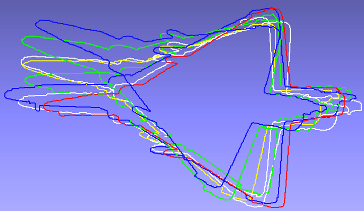
We now apply our method for matching D shapes (Belongie et al. 2002). Without getting into a rigorous analysis, we simply present few results to demonstrate that our method can be used for shape matching. In particular, we wish to match a collection of shapes of a D model without having to compute all pairwise similarities. We have used the models plane, car and bicego from the hmm-gdb database11 1 Download from http://visionlab.uta.edu/shape_data.htm (accessed on Nov, ).. The scans are first centered and arbitrarily labeled. Picky-ICP is then used to estimate the correspondences between successive pairs of scans. Finally, the scans are registered using our method. The results are shown in Figure 8. Notice that the scans do not match perfectly. This is expected since the scans are originally deformed and also because we use only rigid transforms. Nevertheless, the overall matching appears to be reasonably good.


V Multiview Registration
We next use the proposed algorithm for the registration of 3D scans (Sharp et al. 2002). The important consideration here is that the point-to-point correspondences need to be estimated from the scan data. We propose to use two-scan registration for the same which is discussed next.
V-A Correspondence Estimation
As mentioned, the scans extracted from a model are represented using a mesh (Levoy et al. 2005). We treat each scan as a point cloud, where the points are simply the mesh vertices. We first determine which pairs of scans overlap and the correspondences between them. This information is supplied to our registration algorithm. Note that, while we determine the correspondences in a pairwise manner, the registration algorithm takes all the pairwise correspondences into account. To find pairwise correspondences, we can use ICP or its fast variant (Besl and McKay 1992; Rusinkiewicz and Levoy 2001). However, we noticed in our experiments that these are sensitive to outliers. After trying different methods, we found that the correspondences obtained using Picky-ICP Zinßer et al. 2003 give good reconstructions for our registration algorithm. In ICP, multiple points from scan are often assigned to a single point from some target scan . However, the correspondences between and should ideally be one-to-one. In Picky-ICP, the correspondences between and are first estimated as in ICP. Multiple assignments are then resolved by selecting the point in (among several candidates) that is closest to the matching point in (ties are randomly broken). Let be the distances between corresponding points and be their standard deviation. Pairs for which is within a certain factor of are considered as overlapping points, and the remaining points are discarded. In our case, we set the factor as three. We simply used PickyICP as a black box and have not engineered anything on our own. Needless to say, if a better method is used for finding correspondences, the performance of our registration is expected to improve.
V-B Comparisons
. Dataset LRS JRMPC MAICP Our method rot err time rot err time rot err time rot err time Bunny 2.293 0.2 2.384 93.8 1.689 562.0 1.723 0.2 Armadillo 0.309 0.1 1.47 93.4 0.008 521.3 0.051 0.2 Buddha 0.314 0.3 0.926 373.1 0.093 637.4 0.054 0.3 Dragon 0.615 0.2 0.883 150.6 0.015 719.6 0.027 0.2
We report results on four datasets from four datasets: Bunny (Turk and Levoy 1994), Buddha, Dragon (Curless and Levoy 1996) and Armadillo (Krishnamurthy and Levoy 1996). We also compare with some recent methods for multiview registration: MAICP (Govindu and Pooja 2014), LRS (Arrigoni et al. 2016a), and JRMPC (Evangelidis et al. 2014). These methods have already been demonstrated to perform better than Sharp et al. 2002; Torsello et al. 2011; Benjemaa and Schmitt 1999; Williams and Bennamoun 2001; Bernard et al. 2015. Codes for LRS and JRMPC are available online and that of MAICP was provided by the authors. All the competing methods were run using default parameters.


Comparison 1. We first compare the reconstructions using the scans from Stanford dataset. For a fair comparison, we have initialized all methods using PickyICP Zinßer et al. 2003. The reconstruction accuracy is assessed using the error metric in (21). The results are presented in Table V. It is evident that our method performs much better than LRS and JRMPC. The performance is generally comparable to MAICP. Note that the execution time for our method is significantly less. This aspect is especially important when registering several scans. For a visual comparison, the cross-sections of the reconstructions are compared in Table IV. Since the rotation errors for LRS and JRMPC are large, we have only shown the cross-sections for MAICP and our method in Table IV. The number of scans and angular differences are as follows: Bunny ( scans, degree), Armadillo ( scans, degree), Buddha ( scans, degree), and Dragon ( scans, degree). Notice that the cross-section for Buddha is much better for our reconstruction. Following JRMPC, LRS and MAICP, we have tried comparing the convergence rate (of the rotation error) using the following protocol:
- 1.
read the full scans.
- 2.
initialize all methods using PickyICP.
- 3.
run LRS, JRMPC, MAICP and our method on the scans.
- 4.
record the rotation error at each iteration.
The results are shown in Figure 9. Notice that the rotation error decreases quickly for our method and MAICP. The rotation error at convergence is comparable for MAICP and our method. However, the timing is significantly lower in our case. Note that iterations were used for all methods for comparison, though fewer iterations are required for our method and MAICP (cf. Figure 9). Thus only iterations were run MAICP and proposed method in Table V.


Comparison 2. To test robustness, we perturb the individual scans by Gaussian noise and register the scans with all the methods to test for robustness. Some typical results are reported in Figure 7. The performance of the proposed method is generally comparable to MAICP. But again, the timings are significantly less for our method.
Comparison 3. Finally, we carry out experiments with random noise (in the rotations and coordinates) using the following protocol:
- 1.
read the model.
- 2.
center the model by subtracting its centroid and rotate it about the -axis by angles for some fixed (this mimics the collection of point sets using a turn table). For each rotation, the points above the - plane are formed into a point set.
- 3.
perturb the coordinates with additive Gaussian noise.
The trials are carried out times for each noise setting and the resulting errors are averaged. The angle of rotation determines the overlap between successive scans. For all experiments, we fixed to be degrees. We generate scans for Dragon and Buddha. Standard deviation for Gaussian noise is , while the true rotations are randomly perturbed in the range degrees. Reconstruction results from MAICP and our method are shown in Figure 10 for one of the trials. PickyICP is used for initialization in both methods. The averaged rotation error is slightly better for Dragon in our case (our: , MAICP: ). The visual quality also appears to be better for our method (see Figure 10). The timings are sec and min for our method and MAICP. The results are almost identical for Buddha (see Figure 10). Average rotation errors for our method and MAICP are and . However, the timing is significantly lower for our method (our: sec, MAICP: min).


We next simulate scenarios where scans covering the entire model may not be available. For this purpose, we generate scans from Buddha and Armadillo. The scans for Armadillo are perturbed with Gaussian noise having standard deviation . No Gaussian noise is added for Buddha in order to verify reconstruction with just rotation noise. Each scan is randomly rotated in the range degrees. As earlier, we use trials and average the rotation error. PickyICP is used to initialize both methods. Average rotation errors for Buddha are and for our method and MAICP. For Armadillo, the corresponding rotation errors are and respectively. The registration results for one of the trials is shown in Figure 11. Notice that our reconstruction result is much better than MAICP for both models. The possible reason for this is that MAICP uses correspondences between the first and and the last scan. Since full scans are not considered, there are very few overlapping points between them. Again, our method is significantly faster: sec and sec for Buddha and Armadillo compared to min and min for MAICP.
VI Conclusion
We proposed a novel optimization algorithm for registering multiple points sets in a globally consistent fashion using rotations and translations. We empirically analyzed the algorithm and showed that it works well on both simulated and real scan data. An intriguing property of the proposed ADMM solver is that it converges to the global minimum with a good initialization. We could certify this for cases where the global minimum can be computed by some other means, namely, for clean data (where the minimum is zero) and for two scans. We applied the proposed algorithm for 2D shape matching and 3D multiview registration. For the later we compared its performance with recent methods. The reconstruction accuracy of the proposed algorithm is comparable to MAICP but we are much faster. The results also suggest that the overall algorithm is quite robust to noise.
VII Appendix
VII-A Proof of Theorem II.2
It follows from () that . Along with (), we conclude that . Therefore, using () and the spectral theorem for symmetric matrices, we can write
where and is a orthonormal basis of . Define to be
and let , where . By construction, and, in particular,
Therefore, it follows from () that . Furthermore, we conclude from () that for ,
We deduce that for , or . In the latter case, we simply pick a global reflection with , and reassign . This gives us the desired such that (8) holds.
VII-B Proof of Theorem II.4
We can write , where
Let denote matrices in with rank at most . Any can be represented as ,
where and at most of these are positive.
VII-C Proof of Theorem II.5
The projection problem in question is
where we have used the fact that . Since is compact, there exists such that
We claim that . Indeed, consider an arbitrary anti-symmetric matrix such that , and define
Since , it follows that for all ,
Hence,
| (24) |
Since (24) holds for any anti-symmetric , it easily follows that .
Having shown that is symmetric, let , where is a diagonal matrix and . Then
where . Since and commute, they can be diagonalized in the same basis. In particular,
In terms of this representation, we have
| (25) |
Since , (25) is maximum when each . However, since , it follows that
Therefore, if , we must have
| (26) |
since . If , then (25) is maximum when for all . However, if , then it follows from (26) that the maximizer is , and (this is where we use the fact that for all ). The case can be worked out similarly.
References
- Absil et al. (2009) Absil, P.A., Mahony, R., Sepulchre, R., 2009. Optimization Algorithms on Matrix Manifolds. Princeton University Press.
- Ahmed and Chaudhury (2017) Ahmed, S.M., Chaudhury, K.N., 2017. Global multiview registration using non-convex admm. Proc. International Conference on Image Processing (ICIP) , 987–991.
- Arrigoni et al. (2016a) Arrigoni, F., Rossi, B., Fusiello, A., 2016a. Global registration of 3D point sets via LRS decomposition. Proc. European Conference on Computer Vision , 489–504.
- Arrigoni et al. (2016b) Arrigoni, F., Rossi, B., Fusiello, A., 2016b. Spectral synchronization of multiple views in SE(3). SIAM Journal on Imaging Sciences 9, 1963–1990.
- Belongie et al. (2002) Belongie, S., Malik, J., Puzicha, J., 2002. Shape matching and object recognition using shape contexts. IEEE Transactions on Pattern Analysis and Machine Intelligence 24, 509–522.
- Benjemaa and Schmitt (1999) Benjemaa, R., Schmitt, F., 1999. Fast global registration of 3D sampled surfaces using a multi-z-buffer technique. Image and Vision Computing 17, 113–123.
- Bergevin et al. (1996) Bergevin, R., Soucy, M., Gagnon, H., Laurendeau, D., 1996. Towards a general multi-view registration technique. IEEE Transactions on Pattern Analysis and Machine Intelligence 18, 540–547.
- Bernard et al. (2015) Bernard, F., Thunberg, J., Gemmar, P., Hertel, F., Husch, A., Goncalves, J., 2015. A solution for multi-alignment by transformation synchronisation. Proc. IEEE Conference on Computer Vision and Pattern Recognition , 2161–2169.
- Besl and McKay (1992) Besl, P.J., McKay, N.D., 1992. A method for registration of 3-D shapes. IEEE Transactions on Pattern Analysis and Machine Intelligence 14, 239–256.
- Bonarrigo and Signoroni (2011) Bonarrigo, F., Signoroni, A., 2011. An enhanced ‘optimization-on-a-manifold’ framework for global registration of 3D range data. Proc. International Conference on 3D Imaging, Modeling, Processing, Visualization and Transmission , 350–357.
- Bouaziz et al. (2013) Bouaziz, S., Tagliasacchi, A., Pauly, M., 2013. Sparse iterative closest point. Computer Graphics Forum 32, 113–123.
- Boyd et al. (2011) Boyd, S., Parikh, N., Chu, E., Peleato, B., Eckstein, J., 2011. Distributed optimization and statistical learning via the alternating direction method of multipliers. Foundations and Trends® in Machine Learning 3, 1–122.
- Chartrand and Wohlberg (2013) Chartrand, R., Wohlberg, B., 2013. A nonconvex ADMM algorithm for group sparsity with sparse groups. Proc. IEEE International Conference on Acoustics, Speech and Signal Processing , 6009–6013.
- Chaudhury et al. (2015) Chaudhury, K.N., Khoo, Y., Singer, A., 2015. Global registration of multiple point clouds using semidefinite programming. SIAM Journal on Optimization 25, 468–501.
- Chetverikov et al. (2002) Chetverikov, D., Svirko, D., Stepanov, D., Krsek, P., 2002. The trimmed iterative closest point algorithm, in: Object recognition supported by user interaction for service robots, pp. 545–548.
- Curless and Levoy (1996) Curless, B., Levoy, M., 1996. A volumetric method for building complex models from range images , 303–312.
- Diamond et al. (2017) Diamond, S., Takapoui, R., Boyd, S., 2017. A general system for heuristic minimization of convex functions over non-convex sets. Optimization Methods and Software , 1–29.
- Dong et al. (2014) Dong, J., Peng, Y., Ying, S., Hu, Z., 2014. Lietricp: An improvement of trimmed iterative closest point algorithm. Neurocomputing 140, 67–76.
- Du et al. (2011) Du, S., Zhu, J., Zheng, N., Liu, Y., Li, C., 2011. Robust iterative closest point algorithm for registration of point sets with outliers. Optical Engineering 50, 087001.
- Eckart and Young (1936) Eckart, C., Young, G., 1936. The approximation of one matrix by another of lower rank. Psychometrika 1, 211–218.
- Evangelidis et al. (2014) Evangelidis, G.D., Kounades-Bastian, D., Horaud, R., Psarakis, E.Z., 2014. A generative model for the joint registration of multiple point sets. Proc. European Conference on Computer Vision , 109–122.
- Fantoni et al. (2012) Fantoni, S., Castellani, U., Fusiello, A., 2012. Accurate and automatic alignment of range surfaces. Proc. International Conference on 3D Imaging, Modeling, Processing, Visualization and Transmission , 73–80.
- Fusiello et al. (2002) Fusiello, A., Castellani, U., Ronchetti, L., Murino, V., 2002. Model acquisition by registration of multiple acoustic range views. Proc. European Conference on Computer Vision , 558–559.
- Golub and Van Loan (1996) Golub, G.H., Van Loan, C.F., 1996. Matrix Computations. Third ed., The Johns Hopkins University Press.
- Golub and Van Loan (2012) Golub, G.H., Van Loan, C.F., 2012. Matrix Computations. JHU Press.
- Govindu (2004) Govindu, V.M., 2004. Lie-algebraic averaging for globally consistent motion estimation. Proc. IEEE Conference on Computer Vision and Pattern Recognition 1, 684–691.
- Govindu and Pooja (2014) Govindu, V.M., Pooja, A., 2014. On averaging multiview relations for 3D scan registration. IEEE Transactions on Image Processing 23, 1289–1302.
- Guennebaud et al. (2008) Guennebaud, G., Germann, M., Gross, M., 2008. Dynamic sampling and rendering of algebraic point set surfaces. Computer Graphics Forum 27, 653–662.
- Huang and Guibas (2013) Huang, Q.X., Guibas, L., 2013. Consistent shape maps via semidefinite programming. Proc. Computer Graphics Forum 32, 177–186.
- Kabsch (1976) Kabsch, W., 1976. A solution for the best rotation to relate two sets of vectors. Acta Crystallographica Section A: Crystal Physics, Diffraction, Theoretical and General Crystallography 32, 922–923.
- Krishnamurthy and Levoy (1996) Krishnamurthy, V., Levoy, M., 1996. Fitting smooth surfaces to dense polygon meshes, in: Proceedings of the 23rd Annual Conference on Computer Graphics and Interactive Techniques, ACM. pp. 313–324.
- Krishnan et al. (2005) Krishnan, S., Lee, P.Y., Moore, J.B., Venkatasubramanian, S., et al., 2005. Global registration of multiple 3D point sets via optimization-on-a-manifold. Proc. Symposium on Geometry Processing , 187–196.
- Levoy et al. (2005) Levoy, M., Gerth, J., Curless, B., Pull, K., 2005. The Stanford 3D scanning repository. URL http://www-graphics.stanford.edu/data/3dscanrep/ .
- Mateo et al. (2014) Mateo, X., Orriols, X., Binefa, X., 2014. Bayesian perspective for the registration of multiple 3D views. Computer Vision and Image Understanding 118, 84–96.
- Miksik et al. (2014) Miksik, O., Vineet, V., Pérez, P., Torr, P.H., Sévigné, F.C., 2014. Distributed non-convex ADMM-inference in large-scale random fields. Proc. British Machine Vision Conference 2, 7.
- Pennec (1996) Pennec, X., 1996. Multiple registration and mean rigid shapes: Application to the 3D case. Proc. 16th Leeds Annual Statistical Workshop , 178–185.
- Phillips et al. (2007) Phillips, J.M., Liu, R., Tomasi, C., 2007. Outlier robust icp for minimizing fractional rmsd. Sixth International Conference on 3-D Digital Imaging and Modeling , 427–434.
- Raghuramu (2015) Raghuramu, A.C., 2015. Robust multiview registration of 3D surfaces via -norm minimization. Proc. British Machine Vision Conference 145.
- Rusinkiewicz and Levoy (2001) Rusinkiewicz, S., Levoy, M., 2001. Efficient variants of the ICP algorithm. Proc. IEEE Conference on 3-D Digital Imaging and Modeling , 145–152.
- Sharp et al. (2002) Sharp, G.C., Lee, S.W., Wehe, D.K., 2002. Multiview registration of 3D scenes by minimizing error between coordinate frames. Proc. European Conference on Computer Vision , 587–597.
- Toldo et al. (2010) Toldo, R., Beinat, A., Crosilla, F., 2010. Global registration of multiple point clouds embedding the generalized procrustes analysis into an ICP framework. Proc. International Symposium on 3D Data Processing, Visualization and Transmission .
- Torsello et al. (2011) Torsello, A., Rodola, E., Albarelli, A., 2011. Multiview registration via graph diffusion of dual quaternions. Proc. IEEE Conference on Computer Vision and Pattern Recognition , 2441–2448.
- Turk and Levoy (1994) Turk, G., Levoy, M., 1994. Zippered polygon meshes from range images, in: Proceedings of the 21st Annual Conference on Computer Graphics and Interactive Techniques, ACM. pp. 311–318.
- Umeyama (1991) Umeyama, S., 1991. Least-squares estimation of transformation parameters between two point patterns. IEEE Transactions on Pattern Analysis and Machine Intelligence 13, 376–380.
- Wang et al. (2016) Wang, Y., Yin, W., Zeng, J., 2016. Convergence analysis of alternating direction method of multipliers for a family of nonconvex problems. SIAM Journal on Optimization 26, 337–364.
- Wang et al. (2018) Wang, Y., Yin, W., Zeng, J., 2018. Global convergence of ADMM in nonconvex nonsmooth optimization. Journal of Scientific Computing URL: https://doi.org/10.1007/s10915-018-0757-z.
- Williams and Bennamoun (2001) Williams, J., Bennamoun, M., 2001. Simultaneous registration of multiple corresponding point sets. Computer Vision and Image Understanding 81, 117–142.
- Yang et al. (2016) Yang, J., Li, H., Campbell, D., Jia, Y., 2016. Go-ICP: a globally optimal solution to 3D ICP point-set registration. IEEE Transactions on Pattern Analysis and Machine Intelligence 38, 2241–2254.
- Ying et al. (2009a) Ying, S., Peng, J., Du, S., Qiao, H., 2009a. Lie group framework of iterative closest point algorithm for n-D data registration. International Journal of Pattern Recognition and Artificial Intelligence 23, 1201–1220.
- Ying et al. (2009b) Ying, S., Peng, J., Du, S., Qiao, H., 2009b. A scale stretch method based on icp for 3D data registration. IEEE Transactions on Automation Science and Engineering 6, 559–565.
- Zhang et al. (2011) Zhang, L., Choi, S.I., Park, S.Y., 2011. Robust ICP registration using biunique correspondence. Proc. International Conference on 3D Imaging, Modeling, Processing, Visualization and Transmission , 80–85.
- Zinßer et al. (2003) Zinßer, T., Schmidt, J., Niemann, H., 2003. A refined ICP algorithm for robust 3-D correspondence estimation. Proc. IEEE International Conference on Image Processing 2, 695–698.