On Simulating the Proton-Irradiation of O₂ and H₂O Ices Using Astrochemical-type Models,
with Implications for Bulk ReactivityJournal: ApJMONACO (Vasyunin et al. 2017)

Christopher N. Shingledecker OrcID: 0000-0002-5171-7568 Affiliation: Center for Astrochemical Studies Max Planck Intitute for Extraterrestrial Physics Garching, Germany Affiliation: Institute for Theoretical Chemistry University of Stuttgart Pfaffenwaldring 55, 70569 Stuttgart, Germany Corresponding author: Christopher N. Shingledecker Anton Vasyunin Affiliation: Ural Federal University, Ekaterinburg, Russia Affiliation: Visiting Leading Researcher, Engineering Research Institute ’Ventspils International Radio Astronomy Centre’ of Ventspils University of Applied Sciences, Inženieru 101, Ventspils LV-3601, Latvia Eric Herbst Affiliation: Department of Chemistry University of Virginia Charlottesville, VA, USA Affiliation: Department of Astronomy University of Virginia Charlottesville, VA, USA Paola Caselli Affiliation: Center for Astrochemical Studies Max Planck Intitute for Extraterrestrial Physics Garching, Germany

Received January 1, 2018; Revised January 7, 2018; Accepted August 11, 2026

Abstract

Many astrochemical models today explicitly consider the species that comprise the bulk of interstellar dust grain ice-mantles separately from those in the top few monolayers. Bombardment of these ices by ionizing radiation - whether in the form of cosmic rays, stellar winds, or radionuclide emission - represents an astrochemically viable means of driving a rich chemistry even in the bulk of the ice-mantle, now supported by a large body of work in laboratory astrophysics. In this study, using an existing rate equation-based astrochemical code modified to include a method of considering radiation chemistry recently developed by us, we attempted to simulate two such studies in which (a) pure $\text{O}{\vphantom{\text{X}}}_{\smash[t]{\text{2}}}$ ice at 5 K and, (b) pure $\text{H}{\vphantom{\text{X}}}_{\smash[t]{\text{2}}}\text{O}$ ice at 16 K and 77 K, were bombarded by keV $\text{H}{\vphantom{\text{X}}}^{\text{+}}$ ions.

Our aims are twofold: (1) to test the capability of our newly developed method to replicate the results of ice-irradiation experiments, and (2) to determine in such a well-constrained system how bulk chemistry is best handled using the same gas-grain codes that are used to model the interstellar medium (ISM). We find that our modified astrochemical model is able to reproduce both the abundance of $\text{O}{\vphantom{\text{X}}}_{\smash[t]{\text{3}}}$ in the 5 K pure $\text{O}{\vphantom{\text{X}}}_{\smash[t]{\text{2}}}$ ice, as well as both the abundance of $\text{H}{\vphantom{\text{X}}}_{\smash[t]{\text{2}}}\text{O}{\vphantom{\text{X}}}_{\smash[t]{\text{2}}}$ in the 16 K water ice and the previously noted decrease of hydrogen peroxide at higher temperatures. However, these results require the assumption that radicals and other reactive species produced via radiolysis react quickly and non-diffusively with neighbors in the ice.

Keywords:

astrochemistry - molecular processes - cosmic rays

I Introduction

The upcoming launch of the James Webb Space Telescope (JWST) promises to usher in a new astrochemical “ice age” by allowing for the collection of an unprecedented amount of data regarding species frozen onto dust grains in the interstellar medium (ISM). Astrochemical models will surely figure prominently in both interpreting these data as well as in informing future observing proposals. This opportunity, though, calls for models that are equal to the task and, unfortunately, there remain significant uncertainties regarding the chemistry of dust grains and dust grain ice-mantles (Cuppen et al. 2017) - a situation that has given it the dubious reputation of “the last refuge of the scoundrel” (Charnley et al. 1992).

Currently, it is a common practice in modern astrochemical codes to distinguish between species in the top few monolayers of dust grain ice-mantles (the selvedge), and those underneath in the interior (the bulk), though there exists considerable disagreement as to whether, or to what degree, such bulk species are chemically active (Cuppen et al. 2017). The hypothesis that chemistry within the ice-mantle is less significant than in the selvedge rests on the following three main lines of reasoning:

(a)

species in the bulk are more tightly bound,
(b)

a richer chemistry is possible in the selvedge, given the constant exchange of species with the surrounding gas, and
(c)

photo-processes, which further drive chemical reactions, are more efficient in the topmost monolayers.

An implicit assumption behind (a) is that reactions in the bulk occur largely via thermal diffusion, as on surfaces, and thus that reaction rates will be low or negligible for species with high binding energies in cold environments. However, some previous experimental studies strongly suggest that reactions in the bulk can quickly occur among neighboring species, without the need of diffusion (Baragiola et al. 1999; Bennett & Kaiser 2005; Abplanalp et al. 2016; Ghesquière et al. 2018).

Similarly, just as selvedge chemistry is stimulated via photo-processes and interactions with the gas - as noted in (b) and (c) - so too have experiments shown that bombardment by energetic ions, which penetrate solids much more efficiently than photons (Gerakines et al. 2001; Spinks & Woods 1990), causes physicochemical changes that drive a rich chemistry within the ice at low temperatures. This radiation chemistry is quite relevant to the ISM, since ices there are continually bombarded by energetic particles of one kind or another, though typically in the form of cosmic rays (Indriolo & McCall 2013; Rothard et al. 2017), stellar winds (Madey et al. 2002; Hudson & Moore 2001), or radionuclide emission (Cleeves et al. 2013).

Thus, the processing of dust grain ice-mantles by ionizing radiation is a very real phenomenon and the fact that such interactions can lead to the formation of astrochemically interesting, even prebiotic, species makes radiation chemistry very promising from a modeling standpoint (Hudson et al. 2008; Holtom et al. 2005; Kaiser & Roessler 1997; Abplanalp et al. 2016). Until recently, though, the variety and complexity of the underlying microscopic processes have hindered attempts to add radiation-chemical reactions to astrochemical codes (Abplanalp et al. 2016; Shingledecker et al. 2018).

These processes result from collisions between an incoming particle (the primary ion), and species in the target material. Following the formalism of Bohr 1913, it is customary to divide such collisions into two categories, namely, those in which energy is transferred to target nuclei (elastic) or electrons (inelastic). One can therefore express the energy loss per unit path length of the primary ion - called the stopping power - as follows:

\frac{\mathrm{d}E}{\mathrm{d}t}\approx n(S_{\mathrm{n}}+S_{\mathrm{e}})

(1)

where $n$ is the density of the target (cm^-3) and $S_{\mathrm{n}}$ and $S_{\mathrm{e}}$ are, respectively, the so-called nuclear/elastic and electronic/inelastic stopping cross sections (eV-cm²). Inelastic collisions, in turn, can further be divided into those in which target species are ionized or excited. Such ionizations result in the formation of so-called “secondary electrons” which typically have energies under 50 eV and can themselves ionize or excite target species, thereby further propagating the physicochemical effects initiated by the primary ion (Spinks & Woods 1990; Johnson 1990).

Recently in Shingledecker & Herbst 2018 (hereafter, SH), we introduced a method for treating radiation-chemical processes that is simple enough to include in existing astrochemical models, while simultaneously preserving salient features inferred from experimental data. This method was later added to the astrochemical-type Nautilus v1.1 code (Ruaud et al. 2016), and used by us to determine what, if any, effects these new processes would have on cold core models (Shingledecker et al. 2018). Preliminary results from that study indicated that cosmic ray induced reactions could indeed result in enhanced abundances for a number of species, including methyl formate and ethanol, and allowed us to include novel reactions such as insertions (Bergner et al. 2017; Bergantini et al. 2018). However, given the uncertainties sometimes involved in comparing the results of astrochemical models with observations of interstellar environments - particularly in cases where grain-surface chemistry is involved - questions lingered regarding how well astrochemical models were actually simulating irradiation chemistry.

To that end, we have carried out simulations of two different ice irradiation experiments using an existing astrochemical-type model (Vasyunin et al. 2017), modified to include the SH method for treating radiation chemistry. Specifically, we have modeled the bombardment of a 5 K pure $\text{O}{\vphantom{\text{X}}}_{\smash[t]{\text{2}}}$ ice by 100 keV protons as described in Baragiola et al. 1999 as well as that of a pure water ice at both 16 K and 77 K by 200 keV protons, as reported in Gomis et al. 2004a. Doing so has not only afforded us the opportunity to compare how well our simulations replicate the experimental data, but also to directly gauge how well our models perform, more generally, with handling reactions in the bulk ice over a range of temperatures. By thus testing our approaches to ice chemistry in well constrained experimental systems, confidence can be increased in the results of models of much less well constrained interstellar environments.

The rest of the paper is as follows: in §II we discuss details of both the model and chemical network used in this work. In §III our major results are described and their significance is discussed. Finally, our conclusions and suggestions for future work are presented in §IV.

II Model and Network

The basis of this work is the MONACO code, described in Vasyunin et al. 2017, which uses a rate-equation approach for reactions in the gas phase, and the so-called “modified rate-equation” method for reactions on and in dust grain ice mantles (Garrod 2008; Garrod et al. 2009). As in Vasyunin & Herbst 2013 we assume the selvedge, a term for the altered layers near the top of the mantle, is comprised of the top four monolayers of the ice (Vasyunin & Herbst 2013).

We have modified the code to account for irradiation-chemical reactions on and in ice using the SH method, the foundation of which is the assumption that one of the following outcomes is possible upon collision between an energetic particle, the primary ion or a secondary electron, and some target species, $A$ :

A\leadsto A^{+}+e^{-}

(P1)

A\leadsto A^{+}+e^{-}\rightarrow A^{*}\rightarrow B^{*}+C^{*}

(P2)

A\leadsto A^{*}\rightarrow B+C

(P3)

A\leadsto A^{*}

(P4)

where the curly arrow indicates a collision. In processes (P1) and (P2), $A$ is ionized, though with fast charge recombination leading to the formation of suprathermal dissociation products, designated with an asterisk, assumed to occur in (P2). Processes (P3) and (P4) represent collisions in which a suprathermal product is electronically excited directly into some higher state which, in the case of (P3), is assumed to lead to the formation of thermal products. The efficiencies of (P1) - (P4) are characterized by radiochemical yields, called $G$ -values, which give the number of molecules created (or destroyed) per 100 eV transferred to the system from bombarding particles (Dewhurst et al. 1952; Spinks & Woods 1990). A full list of the radiolysis processes used here is given in Table A1 of Appendix A. The yields given there were arrived at through a two-step process where first, initial values were estimated usnig the SH method and subsequently adjusted to improve agreement with the experimental data. It should be noted that, following Shingledecker et al. 2018, we assume the rate of process (P1) is zero, i.e. that all charged species produced in the bulk via ionization are quickly neutralized.

First-order rate coefficients for each radiolysis process are calculated using

k_{\mathrm{rad}}=\left(\frac{G}{100\;\mathrm{eV}}\right)S_{\mathrm{e}}\phi,

(2)

with $\phi$ being the radiation flux and $S_{\mathrm{e}}$ the previously described inelastic/electronic stopping cross section. In this work, we assume the flux to be $1.0\times 10^{11}$ $\text{H}{\vphantom{\text{X}}}^{\text{+}}$ $\mathrm{cm}^{-2}$ $\mathrm{s^{-1}}$ , and use the stopping cross sections given in Table 1.

We assume that, in the bulk, suprathermal species produced via radiolysis rapidly undergo either (a) reaction with a neighbor, or (b) are quenched by the surrounding material. Rate coefficients for the reaction between $A$ and $B$ - where either one could be suprathermal - are calculated using the expression

k_{\mathrm{fast}}=f_{\mathrm{br}}\left[\frac{\nu_{0}^{A}+\nu_{0}^{B}}{{N_{\mathrm{bulk}}}}\right]\mathrm{exp}\left(-\frac{E_{\mathrm{act}}^{AB}}{T_{\mathrm{ice}}}\right),

(3)

where $f_{\mathrm{br}}$ is the branching fraction, $N_{\mathrm{bulk}}$ is the total number of bulk species in the simulated ice, and $E_{\mathrm{act}}^{AB}$ is the activation energy for reaction. Absent other data, we assume here that suprathermal species react barrierlessly. The characteristic vibrational frequency, $\nu^{A}_{0}$ , is given by

\nu_{0}^{A}=\sqrt{\frac{2n_{\mathrm{s}}E^{A}_{\mathrm{D}}}{\pi^{2}m_{A}}},

(4)

with $E^{A}_{\mathrm{D}}$ and $m_{A}$ being the desorption energy and mass of $A$ , respectively, and $n_{\mathrm{s}}$ the phsysisorption site density - here $6.55\times 10^{14}$ cm^-2 (Vasyunin et al. 2017). This characteristic vibrational frequency is also used as the first-order rate coefficient for the quenching of the suprathermal species by the ice. It should be noted that, particularly in water ice, these electronic excitations, also called excitons, may diffuse from the interior of the ice to the selvedge, where they can drive the desorption of species into the gas (Thrower et al. 2011; Marchione et al. 2016). Thus, our assumption that these suprathermal species are rapidly quenched should be seen as a first-order approximation of their real behavior.

As an example of how the above equations are utilized in our code, consider the time-dependent abundance of $B^{*}$ . Assuming $B^{*}$ is produced via the radiolysis of $A$ as in (P2), and destroyed both via quenching and reaction with some other bulk species, $X$ , the rate of change in the number of $B^{*}$ as a function of time can be described by

\frac{d\,N_{B^{*}}}{dt}=k_{\mathrm{rad}}^{\mathrm{\ref{p2}}}N_{A}-\nu_{0}^{B}N_{B^{*}}-k_{\mathrm{fast}}N_{X}N_{B^{*}},

(5)

where the reaction between $B^{*}$ and $X$ is, as with all suprathermal species here, assumed to occur barrierlessly.

Table 1: Physical parameters used in simulations of experiments.

Parameter	Value	Source
$\text{O}{\vphantom{\text{X}}}_{\smash[t]{\text{2}}}$
Temperature	5 K	Baragiola et al. 1999
Density	$5.7\times 10^{22}$ cm^-3	Horl & Kohlbeck 1982
$\text{H}{\vphantom{\text{X}}}^{\text{+}}$ Energy	100 keV	Baragiola et al. 1999
$S_{\mathrm{e}}$	$4.6\times 10^{-14}$ eV cm²	Baragiola et al. 1999
$\text{H}{\vphantom{\text{X}}}_{\smash[t]{\text{2}}}\text{O}$
Temperature	16 K, 77 K	Gomis et al. 2004b
Density	$3.1\times 10^{22}$ cm^-3	Martoňák et al. 2005
$\text{H}{\vphantom{\text{X}}}^{\text{+}}$ Energy	200 keV	Gomis et al. 2004b
$S_{\mathrm{e}}$	$3.3\times 10^{-14}$ eV cm²	Uehara et al. 2000

In order to gauge how well astrochemical models are able to reproduce bulk chemistry, we have run the following three sets of simulations for each experiment considered here using the parameters listed in Table 1:

(a)

a set of models in which thermal radicals and atomic oxygen were assumed to react non-diffusively with neighboring species in the ice with rate coefficients calculated using Eq. (3),
(b)

a set of models in which all bulk rate coefficients were calculated using the standard diffusive formula (Hasegawa et al. 1992) along with diffusion barriers obtained from the desorption energies listed in Table 2 and no tunneling under diffusion barriers for any species, and
(c)

a set of models similar to (b) but with tunneling through diffusion barriers allowed for H, $\text{H}{\vphantom{\text{X}}}_{\smash[t]{\text{2}}}$ , and O.

For the third set of simulations, we treat tunneling under diffusion barriers by H and $\text{H}{\vphantom{\text{X}}}_{\smash[t]{\text{2}}}$ using the standard formalism in Hasegawa et al. 1992 with a barrier width of 1.0 Å. For atomic oxygen, following results from Minissale et al. 2013, we use a desorption energy of 1040 K and a barrier width of 0.7 Å. In all simulations, H and $\text{H}{\vphantom{\text{X}}}_{\smash[t]{\text{2}}}$ were assumed to tunnel through reaction barriers (Tielens & Hagen 1982). The competition mechanism for systems with chemical activation energies (Chang et al. 2007; Herbst & Millar 2008) is used here in all models only for reactions on the surface.

Table 2: Desorption energies for relevant species.

Species	$E_{\mathrm{D}}$ (K)	Source
O	1 660^a^aUsed in models (a) and (b)	He et al. 2015
	1 040^b^bUsed in model (c)	Minissale et al. 2013
$\text{O}{\vphantom{\text{X}}}_{\smash[t]{\text{2}}}$	930	Jing et al. 2012
$\text{O}{\vphantom{\text{X}}}_{\smash[t]{\text{3}}}$	1 833	Jing et al. 2012
H	450	Garrod & Herbst 2006
(Thrower et al. 2011; Marchione et al. 2016) $\text{H}{\vphantom{\text{X}}}_{\smash[t]{\text{2}}}$	430	Garrod & Herbst 2006
OH	2 850	Garrod & Herbst 2006
$\text{H}{\vphantom{\text{X}}}_{\smash[t]{\text{2}}}\text{O}$	5 700	Garrod & Herbst 2006
$\text{HO}{\vphantom{\text{X}}}_{\smash[t]{\text{2}}}$	4 510	$E_{\mathrm{D}}^{\mathrm{O}}+E_{\mathrm{D}}^{\mathrm{OH}}$
$\text{H}{\vphantom{\text{X}}}_{\smash[t]{\text{2}}}\text{O}{\vphantom{\text{X}}}_{\smash[t]{\text{2}}}$	5 700	$E_{\mathrm{D}}^{\mathrm{OH}}+E_{\mathrm{D}}^{\mathrm{OH}}$

Note. — Diffusion barriers in the selvedge were assumed to be $0.5\times E_{\mathrm{D}}$ , while those in the bulk to be $0.7\times E_{\mathrm{D}}$ .

For the chemical network, we used the reactions listed in Table B1 of Appendix B, as well as the neutral-neutral oxygen reactions listed in Table 7 of Shingledecker et al. 2017. In cases where we have been unable to find values for activation energies, we have assumed a barrier of $10^{4}$ K, except for radical-radical reactions, which were assumed to be barrierless. For every thermal reaction of the type given in Table B1, we included variants involving one suprathermal reactant. To illustrate this point, for every reaction of the form $\mathrm{A+B\rightarrow}\;products$ , we include the following suprathermal variants

\mathrm{A^{*}+B\rightarrow}\;products

(R1)

\mathrm{A+B^{*}\rightarrow}\;products.

(R2)

A number of reactions listed in Table B1 have barriers that are quite high for astrochemical networks, but are more common in the combustion-chemical literature from which most are taken. Even though the rates of such reactions involving thermal species will indeed be negligible in our models, the variants involving suprathermal species should be efficient even at the temperatures considered here. For example, even a $40\,000$ K barrier corresponds to only $\sim 3.4$ eV, a realistic energy for an electronically excited suprathermal species.

III Results and Discussion

In order to examine how well astrochemical models using the SH method are capable of reproducing experimental data, as well as to determine the accuracy of bulk chemistry in such codes, we have simulated ice-irradiation systems described in two previous radiation-chemical studies discussed above - the results of which are described below.

III.1 H⁺ Bombardment of Pure O₂ Ice

Figure 1: Results from simulations of an irradiated pure O₂ ice using (a) fast bulk reaction of O, (b) standard bulk rate coefficients based on thermal hopping, and (c) O atom tunneling.

In this system, the only radical used is atomic oxygen, which can be thermal or suprathermal. We first simulated the irradiation of a pure $\text{O}{\vphantom{\text{X}}}_{\smash[t]{\text{2}}}$ ice at 5 K by 100 keV $\text{H}{\vphantom{\text{X}}}^{\text{+}}$ , following the study by Baragiola et al. 1999, which has previously been successfully modeled by us using the much more detailed Monte Carlo code, CIRIS (Shingledecker et al. 2017). An irradiated $\text{O}{\vphantom{\text{X}}}_{\smash[t]{\text{2}}}$ ice is, in many respects, an ideal system for testing simulations of radiation chemistry, given the limited number of possible neutral species, i.e. O, $\text{O}{\vphantom{\text{X}}}_{\smash[t]{\text{2}}}$ , and $\text{O}{\vphantom{\text{X}}}_{\smash[t]{\text{3}}}$ . However, in the Monte Carlo code even this seemingly simple system required a network of $\sim 50$ reactions or processes and involved a level of detail beyond the practical capabilities of rate equations-based astrochemical codes, such as explicitly calculating the tracks of incident ions and secondary electrons or following each ice species on a hop-by-hop basis.

Despite these limitations though, as shown in Fig. 1a, even our simplified approach is capable of reasonably reproducing the concentration of $\text{O}{\vphantom{\text{X}}}_{\smash[t]{\text{3}}}$ as a function of fluence. Here, fluence - the product of the $\text{H}{\vphantom{\text{X}}}^{\text{+}}$ flux and irradiation time - represents the number of ions that have bombarded the ice per cm². As can be seen in Fig. 1, the best results were obtained in model (a), where atomic oxygen is assumed to react non-diffusively in the bulk, yielding excellent agreement between calculated and experimental abundances in the steady stage regime. An analogous assumption was made in our previous Monte Carlo simulations using CIRIS, with similarly good results (Shingledecker et al. 2017). The slight under-prediction of $\text{O}{\vphantom{\text{X}}}_{\smash[t]{\text{3}}}$ at fluences under $\sim 10^{13}$ $\text{H}{\vphantom{\text{X}}}^{\text{+}}$ cm^-1 is likely due to additional processes - such as dissociative electron attachment (DEA) - which are also driven by energetic ion bombardment but not currently considered in this simplified treatment of radiolysis (Arumainayagam et al. 2010). Also noticeable in Fig. 1a is the fact that atomic oxygen abundances remained low throughout the simulation, despite its continuous production from the dissociation of $\text{O}{\vphantom{\text{X}}}_{\smash[t]{\text{2}}}$ and, to a lesser degree, $\text{O}{\vphantom{\text{X}}}_{\smash[t]{\text{3}}}$ .

Comparison with Fig. 1b reveals that model (b), using standard Langmuir-Hinshelwood rate coefficients, is the least accurate. There, though the modeled $\text{O}{\vphantom{\text{X}}}_{\smash[t]{\text{3}}}$ abundance is only a factor of a few lower than the experimental values, an unrealistically large abundance of atomic oxygen is predicted, contrary to what has been suggested by previous studies (Gerakines et al. 1996; Baragiola et al. 1999; Bennett & Kaiser 2005). This buildup is caused by the very slow rates of thermal diffusion reactions at 5 K, given the high atomic oxygen desorption energy of 1660 K (He et al. 2015).

In order to determine the possible effects of quantum tunneling by atomic oxygen through diffusion barriers, as suggested by Minissale et al. 2013, we ran further simulations using their best-fit results of a barrier width of $0.7$ Å and a desorption energy of 1040 K (assuming $E_{\mathrm{b}}=0.5E_{\mathrm{D}}$ ). Tunneling for H and $\text{H}{\vphantom{\text{X}}}_{\smash[t]{\text{2}}}$ is treated using the method of Hasegawa et al. 1992, in which a barrier width of 1 Å is assumed. Comparison of the results of this model, shown in Fig. 1c, with 1b reveals that though agreement between the calculated and experimental ozone abundances is improved, the abundance of atomic oxygen remains too high.

The results of these three models demonstrate that best agreement with experimental data - both the measured $\text{O}{\vphantom{\text{X}}}_{\smash[t]{\text{3}}}$ abundance as well as the inferred low O abundance - is obtained when atomic oxygen is assumed to react quickly in the bulk. We note, however, that the predicted atomic oxygen abundances in model (a) may in fact be somewhat too low, based on the observation by Bennett & Kaiser 2005 of an IR feature associated with an [ $\text{O}{\vphantom{\text{X}}}_{\smash[t]{\text{3}}}$ …O] complex, though no estimate of the atomic oxygen abundance (or an upper limit) was derived. In such irradiated ices, it is likely that some fraction of the oxygen atoms cannot react quickly, either due to trapping by $\text{O}{\vphantom{\text{X}}}_{\smash[t]{\text{3}}}$ or steric effects, in which case their abundance would indeed be greater than that predicted in our models. These effects could be accounted for in the method used here by decreasing the value of the pre-exponential frequency, $\nu_{0}$ , thereby increasing the abundance of O. Here, we use the characteristic vibrational frequency given in Eq. (4) (which typically has a value on the order of $10^{12}$ s^-1) as a rough approximation, though in fact, the value of this parameter can be as low as $10^{-3}$ s^-1 (Theulé et al. 2013), and rate coefficients obtained using (4) should probably be interpreted as upper limits.

III.2 H⁺ Bombardment of Pure H₂O Ice

We next simulated the irradiation of a pure $\text{H}{\vphantom{\text{X}}}_{\smash[t]{\text{2}}}\text{O}$ ice by 200 keV $\text{H}{\vphantom{\text{X}}}^{\text{+}}$ at both 16 and 77 K using the three different bulk chemistry schemes described in Sec. II. Here, in addition to atomic oxygen, we further assume that all radicals in our network – H, OH, and $\text{HO}{\vphantom{\text{X}}}_{\smash[t]{\text{2}}}$ – react quickly in model (a). This system, though substantially more complex than $\text{O}{\vphantom{\text{X}}}_{\smash[t]{\text{2}}}$ , is of greater astronomical interest, given the ubiquity of water ice in planetary bodies (Altwegg et al. 2015; Carlson et al. 2009), as well as interstellar dust grain ice mantles (Gibb et al. 2004).

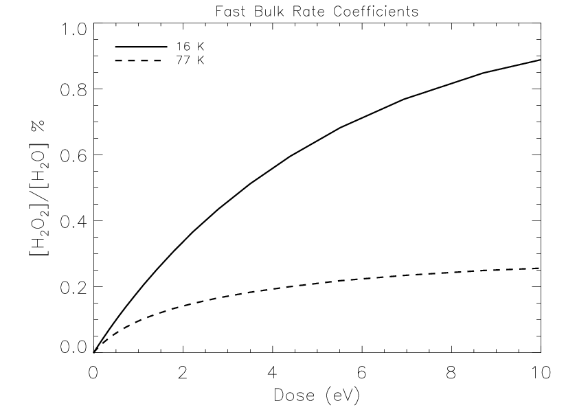
Shown in Fig. 2 are both our calculated $\text{H}{\vphantom{\text{X}}}_{\smash[t]{\text{2}}}\text{O}{\vphantom{\text{X}}}_{\smash[t]{\text{2}}}$ abundances vs proton fluence as well as the approximate steady-state bf experimental values from Gomis et al. 2004a relative to $\text{H}{\vphantom{\text{X}}}_{\smash[t]{\text{2}}}\text{O}$ of $\sim 1.0$ % at 16 K and $0.25$ % at 77 K. As with the pure $\text{O}{\vphantom{\text{X}}}_{\smash[t]{\text{2}}}$ ice, model (a) once again provides the best agreement with experimental data and, notably, is the only one of the three to predict a drop in hydrogen peroxide abundance at higher temperatures. Moore & Hudson 2000, who first detected this trend, speculated that it was due to the reaction

{}\mathrm{OH}{}+{}{}{}\mathrm{H}{\vphantom{\mathrm{X}}}_{\smash[t]{\mathrm{2}}}\mathrm{O}{\vphantom{\mathrm{X}}}_{\smash[t]{\mathrm{2}}}{}\mathrel{\mathop{\makebox[0.0pt]{\rightarrow\displaystyle}}\limits}{}{}{}\mathrm{H}{\vphantom{\mathrm{X}}}_{\smash[t]{\mathrm{2}}}\mathrm{O}{}+{}{}\mathrm{HO}{\vphantom{\mathrm{X}}}_{\smash[t]{\mathrm{2}}}

(R3)

We find that, in agreement with Moore & Hudson 2000, reaction (R3) is indeed behind the drop in $\text{H}{\vphantom{\text{X}}}_{\smash[t]{\text{2}}}\text{O}{\vphantom{\text{X}}}_{\smash[t]{\text{2}}}$ abundance at $\sim 80$ K, since, even though it is assumed that radicals such as OH react quickly, (R3) only becomes competitive at 77 K due to the 755.3 K barrier (Ginovska et al. 2007). In models (b) and (c) the effect of reaction (R3) is reduced by the slow diffusion rates of OH and $\text{H}{\vphantom{\text{X}}}_{\smash[t]{\text{2}}}\text{O}{\vphantom{\text{X}}}_{\smash[t]{\text{2}}}$ . As can be seen in Fig. 3, without the assumption that radicals react quickly in the bulk, OH, in particular, becomes quite abundant in the ice, even at 77 K.

The increase in hydrogen peroxide abundance at 77 K in models (b) and (c) is due to the following reactions:

{}\mathrm{OH}{}+{}{}\mathrm{OH}{}\mathrel{\mathop{\makebox[0.0pt]{\rightarrow\displaystyle}}\limits}{}{}{}\mathrm{H}{\vphantom{\mathrm{X}}}_{\smash[t]{\mathrm{2}}}\mathrm{O}{\vphantom{\mathrm{X}}}_{\smash[t]{\mathrm{2}}}

(R4)

{}\mathrm{H}{}+{}{}\mathrm{HO}{\vphantom{\mathrm{X}}}_{\smash[t]{\mathrm{2}}}{}\mathrel{\mathop{\makebox[0.0pt]{\rightarrow\displaystyle}}\limits}{}{}{}\mathrm{H}{\vphantom{\mathrm{X}}}_{\smash[t]{\mathrm{2}}}\mathrm{O}{\vphantom{\mathrm{X}}}_{\smash[t]{\mathrm{2}}},

(R5)

where here, the higher rate of $\text{H}{\vphantom{\text{X}}}_{\smash[t]{\text{2}}}\text{O}{\vphantom{\text{X}}}_{\smash[t]{\text{2}}}$ formation is due to the increased mobility of the reactants. Enabling quantum tunneling through diffusion barriers, as in model (c), further speeds up the rate of reaction (R5), as well as the formation of the precursor species, $\text{HO}{\vphantom{\text{X}}}_{\smash[t]{\text{2}}}$ , via

{}\mathrm{H}{}+{}{}\mathrm{O}{\vphantom{\mathrm{X}}}_{\smash[t]{\mathrm{2}}}{}\mathrel{\mathop{\makebox[0.0pt]{\rightarrow\displaystyle}}\limits}{}{}\mathrm{HO}{\vphantom{\mathrm{X}}}_{\smash[t]{\mathrm{2}}},

(R6)

thereby contributing to the even higher $\text{H}{\vphantom{\text{X}}}_{\smash[t]{\text{2}}}\text{O}{\vphantom{\text{X}}}_{\smash[t]{\text{2}}}$ abundance at 77 K in model (c) compared with model (b).

We can gain further insights into how closely our simulations are replicating the experiment by examining $G$ ( $\text{H}{\vphantom{\text{X}}}_{\smash[t]{\text{2}}}\text{O}{\vphantom{\text{X}}}_{\smash[t]{\text{2}}}$ ), the radiolytic hydrogen peroxide formation yield. Unfortunately, we cannot simply compare the $G$ -values given in Table A1 with experimentally determined ones directly, since our values are more representative of the immediate creation (or destruction) of target species, i.e. the efficiencies of each of the microscopic radiolytic processes given in (P1)-(P4), than the single effective experimental value, which is sensitive to the temperature-dependent chemistry of the system (Spinks & Woods 1990). However, following the method used in Moore & Hudson 2000, we can estimate what the experimental $G$ -value might be from the slope of a linear fit to the abundance curves in Fig. 5 over the pre-steady-state regime - corresponding to doses of ca. 0-10 eV, where dose is the product of the fluence and $S_{\mathrm{e}}$ . From this, we calculate the yield of H₂O₂ at 16 K to be $0.1$ molecules/100 eV - exactly what was mentioned by Moore & Hudson 2000 as the yield in pure $\text{H}{\vphantom{\text{X}}}_{\smash[t]{\text{2}}}\text{O}$ .

Figure 2: Calculated abundances of

\text{H}{\vphantom{\text{X}}}_{\smash[t]{\text{2}}}\text{O}{\vphantom{\text{X}}}_{\smash[t]{\text{2}}}

versus proton fluence from simulations of a pure

\text{H}{\vphantom{\text{X}}}_{\smash[t]{\text{2}}}\text{O}

ice bombarded by 200 keV

\text{H}{\vphantom{\text{X}}}^{\text{+}}

assuming (a) fast bulk reactions of radicals and atomic oxygen, (b) only thermal bulk diffusion, and (c) diffusion barrier tunneling for H,

\text{H}{\vphantom{\text{X}}}_{\smash[t]{\text{2}}}

, and O. Approximate steady-state hydrogen peroxide abundances from Gomis et al. 2004a at both 16 K and 77 K are represented by the solid, and line-filled boxes, respectively.

Figure 3: Calculated abundances of H, O, OH, and

\text{HO}{\vphantom{\text{X}}}_{\smash[t]{\text{2}}}

versus proton fluence at 16 K (solid lines) and 77 K (dashed lines) from simulations of a pure

\text{H}{\vphantom{\text{X}}}_{\smash[t]{\text{2}}}\text{O}

ice bombarded by 200 keV

\text{H}{\vphantom{\text{X}}}^{\text{+}}

assuming (a) fast bulk reactions of radicals and atomic oxygen, (b) only thermal bulk diffusion, and (c) diffusion barrier tunneling for H,

\text{H}{\vphantom{\text{X}}}_{\smash[t]{\text{2}}}

, and O.

Figure 6: Calculated abundances of

\text{H}{\vphantom{\text{X}}}_{\smash[t]{\text{2}}}

\text{O}{\vphantom{\text{X}}}_{\smash[t]{\text{2}}}

, and

\text{O}{\vphantom{\text{X}}}_{\smash[t]{\text{3}}}

at 16 K (solid line) and 77 K (dashed line) from simulations of a pure

\text{H}{\vphantom{\text{X}}}_{\smash[t]{\text{2}}}\text{O}

ice bombarded by 200 keV

\text{H}{\vphantom{\text{X}}}^{\text{+}}

assuming (a) fast bulk reactions of radicals and atomic oxygen, (b) only thermal bulk diffusion, and (c) diffusion barrier tunneling for H,

\text{H}{\vphantom{\text{X}}}_{\smash[t]{\text{2}}}

, and O.

Shown in Fig. 6 are the abundances of $\text{H}{\vphantom{\text{X}}}_{\smash[t]{\text{2}}}$ , $\text{O}{\vphantom{\text{X}}}_{\smash[t]{\text{2}}}$ , and $\text{O}{\vphantom{\text{X}}}_{\smash[t]{\text{3}}}$ versus fluence. In model (a), the abundance of $\text{O}{\vphantom{\text{X}}}_{\smash[t]{\text{2}}}$ at 16 K is kept low because of destruction via (R6) to form $\text{HO}{\vphantom{\text{X}}}_{\smash[t]{\text{2}}}$ but increases at 77 K due, in part, to more efficient formation via

{}\mathrm{HO}{\vphantom{\mathrm{X}}}_{\smash[t]{\mathrm{2}}}{}+{}{}\mathrm{O}{\vphantom{\mathrm{X}}}_{\smash[t]{\mathrm{3}}}{}\mathrel{\mathop{\makebox[0.0pt]{\rightarrow\displaystyle}}\limits}{}{}\mathrm{O}{\vphantom{\mathrm{X}}}_{\smash[t]{\mathrm{2}}}{}+{}{}\mathrm{O}{\vphantom{\mathrm{X}}}_{\smash[t]{\mathrm{2}}}{}+{}{}\mathrm{OH}.

(R7)

which has a small barrier of 490 K Burkholder et al. 2014. Similarly, the increase in molecular oxygen abundance at 77 K in model (c) is further driven by

{}\mathrm{OH}{}+{}{}\mathrm{HO}{\vphantom{\mathrm{X}}}_{\smash[t]{\mathrm{2}}}{}\mathrel{\mathop{\makebox[0.0pt]{\rightarrow\displaystyle}}\limits}{}{}{}\mathrm{H}{\vphantom{\mathrm{X}}}_{\smash[t]{\mathrm{2}}}\mathrm{O}{}+{}{}\mathrm{O}{\vphantom{\mathrm{X}}}_{\smash[t]{\mathrm{2}}}

(R8)

where the abundances of OH and $\text{HO}{\vphantom{\text{X}}}_{\smash[t]{\text{2}}}$ are enhanced relative to model (b) because of the effects of* quantum tunneling through diffusion barriers by H, $\text{H}{\vphantom{\text{X}}}_{\smash[t]{\text{2}}}$ , and O - as shown in Fig. 3. The decreased abundance of these radicals at 77 K in model (b), combined with destruction with atomic oxygen, leads to the drop in [ $\text{O}{\vphantom{\text{X}}}_{\smash[t]{\text{2}}}$ ] in Fig. 6b.

Unfortunately, comparison of our $\text{O}{\vphantom{\text{X}}}_{\smash[t]{\text{2}}}$ results with experimental data, as with $\text{H}{\vphantom{\text{X}}}_{\smash[t]{\text{2}}}\text{O}{\vphantom{\text{X}}}_{\smash[t]{\text{2}}}$ , is complicated by the fact that homonuclear diatomic molecules, lacking permanent dipoles, are IR inactive. Thus, their abundances cannot be measured using standard techniques, such as Fourier Transform Infrared Spectroscoppy (FTIR). Nevertheless, it is well known that $\text{H}{\vphantom{\text{X}}}_{\smash[t]{\text{2}}}$ and $\text{O}{\vphantom{\text{X}}}_{\smash[t]{\text{2}}}$ form during water ice radiolysis based on analysis of both sputtering products as well as post-irradiation temperature-programmed desorption (TPD) of the ice via mass spectrometry (Johnson & Quickenden 1997; Teolis et al. 2017). In principle, though, such measurements should be possible using Raman techniques (Rothard et al. 2017) and would be of great value, in part, by enabling us to further refine both our radiochemical yields and chemical network. Interest in constraining $\text{O}{\vphantom{\text{X}}}_{\smash[t]{\text{2}}}$ abundances in irradiated water was recently renewed following its detection in the coma of comet 67P/C-G by Bieler et al. 2015. As can be seen in Fig. 6, the maximum abundance of $\text{O}{\vphantom{\text{X}}}_{\smash[t]{\text{2}}}$ with respect to water achieved here is $\sim 0.1$ % in model (a) at 77 K, a value which increased only negligibly at still higher temperatures. Thus, our models predict that the radiolysis of pure $\text{H}{\vphantom{\text{X}}}_{\smash[t]{\text{2}}}\text{O}$ ice is not the dominant mechanism behind the $\sim 3.8$ % $\text{O}{\vphantom{\text{X}}}_{\smash[t]{\text{2}}}$ abundances relative to water measured by Rosetta (Bieler et al. 2015). In that study, moreover, no evidence for ozone was found, though an upper limit of $1\times 10^{-4}$ % relative to water was established. Interestingly, only in model (a) are the ozone abundances predicted to remain below this limit, even at 77 K.

IV Conclusions & Outlook

In this work, we have simulated the bombardment of pure $\text{O}{\vphantom{\text{X}}}_{\smash[t]{\text{2}}}$ and $\text{H}{\vphantom{\text{X}}}_{\smash[t]{\text{2}}}\text{O}$ ices by energetic protons using a general rate-equation-based astrochemical code, modified to include radiation-chemical processes using the SH method. These models were carried out with the MONACO program (Vasyunin et al. 2017), and a network consisting of the radiolysis processes listed in Table A1 of Appendix A and the reactions noted in Appendix B. As illustrated in Figs. 1 and 2, we were able to qualitatively reproduce both the abundance of $\text{O}{\vphantom{\text{X}}}_{\smash[t]{\text{3}}}$ in pure $\text{O}{\vphantom{\text{X}}}_{\smash[t]{\text{2}}}$ (Baragiola et al. 1999) and $\text{H}{\vphantom{\text{X}}}_{\smash[t]{\text{2}}}\text{O}{\vphantom{\text{X}}}_{\smash[t]{\text{2}}}$ in pure $\text{H}{\vphantom{\text{X}}}_{\smash[t]{\text{2}}}\text{O}$ (Gomis et al. 2004a) utilizing the radiochemical processes given in Table A1. Thus validated, these processes, along with the reactions given in Table B1, can be added to existing chemical networks in order to better account for physicochemical effects caused by cosmic ray bombardment of dust grain ice-mantles.

Moreover, by simulating well-constrained experiments rather than interstellar environments we have been afforded a unique opportunity to compare the accuracy and physical realism of several approaches to modeling bulk chemistry over a variety of temperatures relevant to the ISM. As reported here, we have found that the standard approaches to bulk chemistry based on thermal diffusion or quantum tunneling through diffusion barriers did more poorly at reproducing the experimental data - particularly at low temperatures - than our model in which radicals and atomic oxygen were assumed to react quickly with neighboring species in the ice. This finding is in agreement with recent experiments by Ghesquière et al. 2018, who found no evidence for true bulk diffusion.

Regrettably, despite the large body of work in laboratory astrophysics on the irradiation of interstellar ice-analogues, it has not been possible, until recently, to incorporate many of the results of these experiments into astrochemical codes (Shingledecker et al. 2018). However, our work presented here shows that not only can such models simulate radiation-chemical reactions, they might even be fruitfully used as a replacement for the simpler kinetic models sometimes employed (e.g. Gomis et al. 2004b; Baragiola et al. 1999) in understanding and analyzing experimental data.

In summary, this study represents an attempt to shrink the existing gap between experiments and models, an increasingly urgent task in light of the upcoming launch of JWST. However, there is ample opportunity for even further refinements to our approach by, for example, considering the effects of the implantation and subsequent reactions of the bombarding $\text{H}{\vphantom{\text{X}}}^{\text{+}}$ ions, of ice heating along the particle track, or of the effects caused by the nuclear/elastic component of the stopping, which begins to dominate over the electronic/inelastic component considered here at lower particle energies (Spinks & Woods 1990). In addition to the synthesis of molecules, charged particle bombardment is well known to drive the non-thermal desorption of even large molecules such as benzene (Thrower et al. 2011; Marchione et al. 2016). From experiments it is known that, particularly in water ice, excitons migrating to the surface represent one such mechanism that can stimulate this desorption. Given lingering questions about how molecules formed in dust-grain ice mantles are introduced into the surrounding gas in cold environments, future improvements to our approach in this area are warranted. Finally, experiments in which the abundances of multiple species are followed during irradiation would further advance our knowledge of radiation-chemical processes in ices and help to reduce uncertainties in future modeling research. In particular, Raman spectroscopic analysis - where even the behavior of IR-inactive species like $\text{O}{\vphantom{\text{X}}}_{\smash[t]{\text{2}}}$ could be monitored - represents a powerful, yet perhaps underutilised, technique that should be considered in future studies.

CNS gratefully acknowledges the support of the Alexander von Humboldt Foundation. EH acknowledges the support of the National Science Foundation through grant AST-1514844. AV acknowledges the support of the Russian Science Foundation through grant 18-12-00351.

Appendix A Radiolysis Processes

The radiolysis processes and radiochemical yields used here are listed in Table A1.

Table A1: Radiolysis reactions, branching fractions, and yields ( G-values) used in this work

Process	$f_{\mathrm{br}}$	$G$ -value^a^aGiven in molecules/100 eV	Type
$\text{H}{\vphantom{\text{X}}}_{\smash[t]{\text{2}}}\text{O}$
$\mathrm{H_{2}O\leadsto OH^{}+H^{}}$	0.9	$2.57\times 10^{-1}$	I
$\mathrm{H_{2}O\leadsto O^{}+H_{2}^{}}$	0.1	$2.57\times 10^{-1}$	I
$\mathrm{H_{2}O\leadsto OH+H}$	0.9	$1.58\times 10^{-1}$	II
$\mathrm{H_{2}O\leadsto O+H_{2}}$	0.1	$1.58\times 10^{-1}$	II
$\mathrm{H_{2}O\leadsto H_{2}O^{*}}$	1.0	$1.58\times 10^{-1}$	III
$\text{O}{\vphantom{\text{X}}}_{\smash[t]{\text{2}}}$
$\mathrm{O_{2}\leadsto O^{}+O^{}}$	1.0	$6.81\times 10^{0}$	I
$\mathrm{O_{2}\leadsto O+O}$	1.0	$2.91\times 10^{0}$	II
$\mathrm{O_{2}\leadsto O_{2}^{*}}$	1.0	$2.91\times 10^{0}$	III
$\text{O}{\vphantom{\text{X}}}_{\smash[t]{\text{3}}}$
$\mathrm{O_{3}\leadsto O_{2}^{}+O^{}}$	1.0	$5.57\times 10^{1}$	I
$\mathrm{O_{3}\leadsto O_{2}+O}$	1.0	$1.80\times 10^{1}$	II
$\mathrm{O_{3}\leadsto O_{3}^{*}}$	1.0	$1.80\times 10^{1}$	III
$\text{HO}{\vphantom{\text{X}}}_{\smash[t]{\text{2}}}$
$\mathrm{HO_{2}\leadsto O^{}+OH^{}}$	0.5	$3.70\times 10^{0}$	I
$\mathrm{HO_{2}\leadsto H^{}+O_{2}^{}}$	0.5	$3.70\times 10^{0}$	I
$\mathrm{HO_{2}\leadsto O+OH}$	0.5	$3.71\times 10^{0}$	II
$\mathrm{HO_{2}\leadsto H+O_{2}}$	0.5	$3.71\times 10^{0}$	II
$\mathrm{HO_{2}\leadsto HO_{2}^{*}}$	1.0	$3.71\times 10^{0}$	III
$\text{H}{\vphantom{\text{X}}}_{\smash[t]{\text{2}}}\text{O}{\vphantom{\text{X}}}_{\smash[t]{\text{2}}}$
$\mathrm{H_{2}O_{2}\leadsto OH^{}+OH^{}}$	0.5	$5.10\times 10^{1}$	I
$\mathrm{H_{2}O_{2}\leadsto H^{}+HO_{2}^{}}$	0.5	$5.10\times 10^{1}$	I
$\mathrm{H_{2}O_{2}\leadsto OH+OH}$	0.5	$4.13\times 10^{1}$	II
$\mathrm{H_{2}O_{2}\leadsto H+HO_{2}}$	0.5	$4.13\times 10^{1}$	II
$\mathrm{H_{2}O_{2}\leadsto H_{2}O_{2}^{*}}$	1.0	$4.13\times 10^{1}$	III
O
$\mathrm{O\leadsto O^{*}}$	1.0	$3.70\times 10^{0}$	I
$\mathrm{O\leadsto O^{*}}$	1.0	$1.93\times 10^{0}$	III
$\text{H}{\vphantom{\text{X}}}_{\smash[t]{\text{2}}}$
$\mathrm{H_{2}\leadsto H^{}+H^{}}$	1.0	$3.70\times 10^{1}$	I
$\mathrm{H_{2}\leadsto H+H}$	1.0	$1.02\times 10^{1}$	II
$\mathrm{H_{2}\leadsto H_{2}^{*}}$	1.0	$1.02\times 10^{1}$	III
OH
$\mathrm{OH\leadsto O^{}+H^{}}$	1.0	$3.70\times 10^{0}$	I
$\mathrm{OH\leadsto O+H}$	1.0	$5.66\times 10^{0}$	II
$\mathrm{OH\leadsto OH^{*}}$	1.0	$5.66\times 10^{0}$	III

Note. — Following Shingledecker et al. 2018 we use Type I to indicate process (P2), Type II process (P3), and Type III process (P4).

Appendix B Chemical Network

The chemical network used in this work consists of the reactions listed in Table B1, as well as the neutral-neutral reactions in Table 7 of Shingledecker et al. 2017.

Table B1: Solid-phase reactions used in water simulations

Reaction	$E_{\mathrm{A}}$ (K)	$f_{\mathrm{br}}$	Source
H + H ${}\mathrel{\mathop{\makebox[0.0pt]{\rightarrow\displaystyle}}\limits}{}$ $\text{H}{\vphantom{\text{X}}}_{\smash[t]{\text{2}}}$	0	1.0	Wakelam et al. 2015
H + $\text{H}{\vphantom{\text{X}}}_{\smash[t]{\text{2}}}$ ${}\mathrel{\mathop{\makebox[0.0pt]{\rightarrow\displaystyle}}\limits}{}$ $\text{H}{\vphantom{\text{X}}}_{\smash[t]{\text{2}}}$ + H	1 900	1.0	Cohen et al. 1992
H + O ${}\mathrel{\mathop{\makebox[0.0pt]{\rightarrow\displaystyle}}\limits}{}$ OH	0	1.0	Atkinson et al. 2004
H + $\text{O}{\vphantom{\text{X}}}_{\smash[t]{\text{2}}}$ ${}\mathrel{\mathop{\makebox[0.0pt]{\rightarrow\displaystyle}}\limits}{}$ $\text{HO}{\vphantom{\text{X}}}_{\smash[t]{\text{2}}}$	0	1.0	JL
H + $\text{O}{\vphantom{\text{X}}}_{\smash[t]{\text{3}}}$ ${}\mathrel{\mathop{\makebox[0.0pt]{\rightarrow\displaystyle}}\limits}{}$ $\text{O}{\vphantom{\text{X}}}_{\smash[t]{\text{2}}}$ + OH	450	1.0	Tielens & Hagen 1982
H + OH ${}\mathrel{\mathop{\makebox[0.0pt]{\rightarrow\displaystyle}}\limits}{}$ $\text{H}{\vphantom{\text{X}}}_{\smash[t]{\text{2}}}\text{O}$	0	1.0	Atkinson et al. 2004
H + $\text{H}{\vphantom{\text{X}}}_{\smash[t]{\text{2}}}\text{O}$ ${}\mathrel{\mathop{\makebox[0.0pt]{\rightarrow\displaystyle}}\limits}{}$ OH + $\text{H}{\vphantom{\text{X}}}_{\smash[t]{\text{2}}}$	9 700	1.0	Baulch et al. 1992
H + $\text{HO}{\vphantom{\text{X}}}_{\smash[t]{\text{2}}}$ ${}\mathrel{\mathop{\makebox[0.0pt]{\rightarrow\displaystyle}}\limits}{}$ O + $\text{H}{\vphantom{\text{X}}}_{\smash[t]{\text{2}}}\text{O}$	0	0.0194	Atkinson et al. 2004
H + $\text{HO}{\vphantom{\text{X}}}_{\smash[t]{\text{2}}}$ ${}\mathrel{\mathop{\makebox[0.0pt]{\rightarrow\displaystyle}}\limits}{}$ $\text{O}{\vphantom{\text{X}}}_{\smash[t]{\text{2}}}$ + $\text{H}{\vphantom{\text{X}}}_{\smash[t]{\text{2}}}$	0	0.0857	Atkinson et al. 2004
H + $\text{HO}{\vphantom{\text{X}}}_{\smash[t]{\text{2}}}$ ${}\mathrel{\mathop{\makebox[0.0pt]{\rightarrow\displaystyle}}\limits}{}$ $\text{H}{\vphantom{\text{X}}}_{\smash[t]{\text{2}}}\text{O}{\vphantom{\text{X}}}_{\smash[t]{\text{2}}}$	0	0.0894	Atkinson et al. 2004
H + $\text{H}{\vphantom{\text{X}}}_{\smash[t]{\text{2}}}\text{O}{\vphantom{\text{X}}}_{\smash[t]{\text{2}}}$ ${}\mathrel{\mathop{\makebox[0.0pt]{\rightarrow\displaystyle}}\limits}{}$ $\text{H}{\vphantom{\text{X}}}_{\smash[t]{\text{2}}}\text{O}$ + OH	1 400	0.999	Baulch et al. 1992
H + $\text{H}{\vphantom{\text{X}}}_{\smash[t]{\text{2}}}\text{O}{\vphantom{\text{X}}}_{\smash[t]{\text{2}}}$ ${}\mathrel{\mathop{\makebox[0.0pt]{\rightarrow\displaystyle}}\limits}{}$ $\text{HO}{\vphantom{\text{X}}}_{\smash[t]{\text{2}}}$ + $\text{H}{\vphantom{\text{X}}}_{\smash[t]{\text{2}}}$	1 900	0.0006	Baulch et al. 1992
$\text{H}{\vphantom{\text{X}}}_{\smash[t]{\text{2}}}$ + O ${}\mathrel{\mathop{\makebox[0.0pt]{\rightarrow\displaystyle}}\limits}{}$ $\text{H}{\vphantom{\text{X}}}_{\smash[t]{\text{2}}}\text{O}$	9 700	1.0	Javoy et al. 2003
$\text{H}{\vphantom{\text{X}}}_{\smash[t]{\text{2}}}$ + $\text{O}{\vphantom{\text{X}}}_{\smash[t]{\text{2}}}$ ${}\mathrel{\mathop{\makebox[0.0pt]{\rightarrow\displaystyle}}\limits}{}$ $\text{HO}{\vphantom{\text{X}}}_{\smash[t]{\text{2}}}$ + H	28 000	1.0	Karkach & Osherov 1999
$\text{H}{\vphantom{\text{X}}}_{\smash[t]{\text{2}}}$ + $\text{O}{\vphantom{\text{X}}}_{\smash[t]{\text{3}}}$ ${}\mathrel{\mathop{\makebox[0.0pt]{\rightarrow\displaystyle}}\limits}{}$ OH + $\text{O}{\vphantom{\text{X}}}_{\smash[t]{\text{2}}}$	10 000	1.0	See text
$\text{H}{\vphantom{\text{X}}}_{\smash[t]{\text{2}}}$ + OH ${}\mathrel{\mathop{\makebox[0.0pt]{\rightarrow\displaystyle}}\limits}{}$ $\text{H}{\vphantom{\text{X}}}_{\smash[t]{\text{2}}}\text{O}$ + H	1 800	1.0	Burkholder et al. 2014
$\text{H}{\vphantom{\text{X}}}_{\smash[t]{\text{2}}}$ + $\text{H}{\vphantom{\text{X}}}_{\smash[t]{\text{2}}}\text{O}$ ${}\mathrel{\mathop{\makebox[0.0pt]{\rightarrow\displaystyle}}\limits}{}$ $\text{H}{\vphantom{\text{X}}}_{\smash[t]{\text{2}}}\text{O}$ + H	10 000	1.0	See text
$\text{H}{\vphantom{\text{X}}}_{\smash[t]{\text{2}}}$ + $\text{HO}{\vphantom{\text{X}}}_{\smash[t]{\text{2}}}$ ${}\mathrel{\mathop{\makebox[0.0pt]{\rightarrow\displaystyle}}\limits}{}$ $\text{H}{\vphantom{\text{X}}}_{\smash[t]{\text{2}}}\text{O}{\vphantom{\text{X}}}_{\smash[t]{\text{2}}}$ + H	13 000	1.0	Tsang & Hampson 1986
$\text{H}{\vphantom{\text{X}}}_{\smash[t]{\text{2}}}$ + $\text{H}{\vphantom{\text{X}}}_{\smash[t]{\text{2}}}\text{O}{\vphantom{\text{X}}}_{\smash[t]{\text{2}}}$ ${}\mathrel{\mathop{\makebox[0.0pt]{\rightarrow\displaystyle}}\limits}{}$ $\text{H}{\vphantom{\text{X}}}_{\smash[t]{\text{2}}}$ + OH + OH	10 000	1.0	See text
O + $\text{O}{\vphantom{\text{X}}}_{\smash[t]{\text{2}}}$ ${}\mathrel{\mathop{\makebox[0.0pt]{\rightarrow\displaystyle}}\limits}{}$ $\text{O}{\vphantom{\text{X}}}_{\smash[t]{\text{3}}}$	180	1.0	Benderskii & Wight 1996
O + OH ${}\mathrel{\mathop{\makebox[0.0pt]{\rightarrow\displaystyle}}\limits}{}$ $\text{HO}{\vphantom{\text{X}}}_{\smash[t]{\text{2}}}$	0	1.0	Atkinson et al. 2004
O + $\text{H}{\vphantom{\text{X}}}_{\smash[t]{\text{2}}}\text{O}$ ${}\mathrel{\mathop{\makebox[0.0pt]{\rightarrow\displaystyle}}\limits}{}$ $\text{H}{\vphantom{\text{X}}}_{\smash[t]{\text{2}}}\text{O}{\vphantom{\text{X}}}_{\smash[t]{\text{2}}}$	8 800	1.0	Karkach & Osherov 1999
O + $\text{HO}{\vphantom{\text{X}}}_{\smash[t]{\text{2}}}$ ${}\mathrel{\mathop{\makebox[0.0pt]{\rightarrow\displaystyle}}\limits}{}$ $\text{O}{\vphantom{\text{X}}}_{\smash[t]{\text{2}}}$ + OH	0	1.0	M84
O + $\text{H}{\vphantom{\text{X}}}_{\smash[t]{\text{2}}}\text{O}{\vphantom{\text{X}}}_{\smash[t]{\text{2}}}$ ${}\mathrel{\mathop{\makebox[0.0pt]{\rightarrow\displaystyle}}\limits}{}$ OH + $\text{HO}{\vphantom{\text{X}}}_{\smash[t]{\text{2}}}$	2 000	1.0	Atkinson et al. 2004
$\text{O}{\vphantom{\text{X}}}_{\smash[t]{\text{2}}}$ + OH ${}\mathrel{\mathop{\makebox[0.0pt]{\rightarrow\displaystyle}}\limits}{}$ $\text{HO}{\vphantom{\text{X}}}_{\smash[t]{\text{2}}}$ + O	25 000	1.0	Srinivasan et al. 2005
$\text{O}{\vphantom{\text{X}}}_{\smash[t]{\text{2}}}$ + $\text{H}{\vphantom{\text{X}}}_{\smash[t]{\text{2}}}\text{O}$ ${}\mathrel{\mathop{\makebox[0.0pt]{\rightarrow\displaystyle}}\limits}{}$ $\text{HO}{\vphantom{\text{X}}}_{\smash[t]{\text{2}}}$ + OH	37 000	1.0	Mayer & Schieler 1968
$\text{O}{\vphantom{\text{X}}}_{\smash[t]{\text{2}}}$ + $\text{HO}{\vphantom{\text{X}}}_{\smash[t]{\text{2}}}$ ${}\mathrel{\mathop{\makebox[0.0pt]{\rightarrow\displaystyle}}\limits}{}$ $\text{O}{\vphantom{\text{X}}}_{\smash[t]{\text{3}}}$ + OH	10 000	1.0	See text
$\text{O}{\vphantom{\text{X}}}_{\smash[t]{\text{2}}}$ + $\text{H}{\vphantom{\text{X}}}_{\smash[t]{\text{2}}}\text{O}{\vphantom{\text{X}}}_{\smash[t]{\text{2}}}$ ${}\mathrel{\mathop{\makebox[0.0pt]{\rightarrow\displaystyle}}\limits}{}$ $\text{HO}{\vphantom{\text{X}}}_{\smash[t]{\text{2}}}$ + $\text{HO}{\vphantom{\text{X}}}_{\smash[t]{\text{2}}}$	18 000	1.0	Donaldson & Francisco 2003
$\text{O}{\vphantom{\text{X}}}_{\smash[t]{\text{3}}}$ + OH ${}\mathrel{\mathop{\makebox[0.0pt]{\rightarrow\displaystyle}}\limits}{}$ $\text{HO}{\vphantom{\text{X}}}_{\smash[t]{\text{2}}}$ + $\text{O}{\vphantom{\text{X}}}_{\smash[t]{\text{2}}}$	940	1.0	Atkinson et al. 2004
$\text{O}{\vphantom{\text{X}}}_{\smash[t]{\text{3}}}$ + $\text{H}{\vphantom{\text{X}}}_{\smash[t]{\text{2}}}\text{O}$ ${}\mathrel{\mathop{\makebox[0.0pt]{\rightarrow\displaystyle}}\limits}{}$ $\text{H}{\vphantom{\text{X}}}_{\smash[t]{\text{2}}}\text{O}{\vphantom{\text{X}}}_{\smash[t]{\text{2}}}$ + $\text{O}{\vphantom{\text{X}}}_{\smash[t]{\text{2}}}$	10 000	1.0	See text
$\text{O}{\vphantom{\text{X}}}_{\smash[t]{\text{3}}}$ + $\text{HO}{\vphantom{\text{X}}}_{\smash[t]{\text{2}}}$ ${}\mathrel{\mathop{\makebox[0.0pt]{\rightarrow\displaystyle}}\limits}{}$ $\text{O}{\vphantom{\text{X}}}_{\smash[t]{\text{2}}}$ + $\text{O}{\vphantom{\text{X}}}_{\smash[t]{\text{2}}}$ + OH	490	1.0	Burkholder et al. 2014
$\text{O}{\vphantom{\text{X}}}_{\smash[t]{\text{3}}}$ + $\text{H}{\vphantom{\text{X}}}_{\smash[t]{\text{2}}}\text{O}{\vphantom{\text{X}}}_{\smash[t]{\text{2}}}$ ${}\mathrel{\mathop{\makebox[0.0pt]{\rightarrow\displaystyle}}\limits}{}$ $\text{O}{\vphantom{\text{X}}}_{\smash[t]{\text{2}}}$ + $\text{O}{\vphantom{\text{X}}}_{\smash[t]{\text{2}}}$ + $\text{H}{\vphantom{\text{X}}}_{\smash[t]{\text{2}}}\text{O}$	10 000	1.0	See text
OH + OH ${}\mathrel{\mathop{\makebox[0.0pt]{\rightarrow\displaystyle}}\limits}{}$ $\text{H}{\vphantom{\text{X}}}_{\smash[t]{\text{2}}}\text{O}{\vphantom{\text{X}}}_{\smash[t]{\text{2}}}$	0	1.0	Atkinson et al. 2004
OH + $\text{H}{\vphantom{\text{X}}}_{\smash[t]{\text{2}}}\text{O}$ ${}\mathrel{\mathop{\makebox[0.0pt]{\rightarrow\displaystyle}}\limits}{}$ $\text{H}{\vphantom{\text{X}}}_{\smash[t]{\text{2}}}\text{O}{\vphantom{\text{X}}}_{\smash[t]{\text{2}}}$ + H	40 000	0.5	Lamberts & Kästner 2017
OH + $\text{H}{\vphantom{\text{X}}}_{\smash[t]{\text{2}}}\text{O}$ ${}\mathrel{\mathop{\makebox[0.0pt]{\rightarrow\displaystyle}}\limits}{}$ $\text{H}{\vphantom{\text{X}}}_{\smash[t]{\text{2}}}\text{O}$ + OH	2 100	0.5	Uchimaru et al. 2003
OH + $\text{HO}{\vphantom{\text{X}}}_{\smash[t]{\text{2}}}$ ${}\mathrel{\mathop{\makebox[0.0pt]{\rightarrow\displaystyle}}\limits}{}$ $\text{H}{\vphantom{\text{X}}}_{\smash[t]{\text{2}}}\text{O}$ + $\text{O}{\vphantom{\text{X}}}_{\smash[t]{\text{2}}}$	0	1.0	Schwab et al. 1989
OH + $\text{H}{\vphantom{\text{X}}}_{\smash[t]{\text{2}}}\text{O}{\vphantom{\text{X}}}_{\smash[t]{\text{2}}}$ ${}\mathrel{\mathop{\makebox[0.0pt]{\rightarrow\displaystyle}}\limits}{}$ $\text{H}{\vphantom{\text{X}}}_{\smash[t]{\text{2}}}\text{O}$ + $\text{HO}{\vphantom{\text{X}}}_{\smash[t]{\text{2}}}$	760	1.0	Buszek et al. 2012
$\text{H}{\vphantom{\text{X}}}_{\smash[t]{\text{2}}}\text{O}$ + $\text{HO}{\vphantom{\text{X}}}_{\smash[t]{\text{2}}}$ ${}\mathrel{\mathop{\makebox[0.0pt]{\rightarrow\displaystyle}}\limits}{}$ $\text{H}{\vphantom{\text{X}}}_{\smash[t]{\text{2}}}\text{O}{\vphantom{\text{X}}}_{\smash[t]{\text{2}}}$ + OH	17 000	1.0	Lloyd 1974
$\text{H}{\vphantom{\text{X}}}_{\smash[t]{\text{2}}}\text{O}$ + $\text{H}{\vphantom{\text{X}}}_{\smash[t]{\text{2}}}\text{O}{\vphantom{\text{X}}}_{\smash[t]{\text{2}}}$ ${}\mathrel{\mathop{\makebox[0.0pt]{\rightarrow\displaystyle}}\limits}{}$ OH + OH + $\text{H}{\vphantom{\text{X}}}_{\smash[t]{\text{2}}}\text{O}$	10 000	1.0	See text
$\text{HO}{\vphantom{\text{X}}}_{\smash[t]{\text{2}}}$ + $\text{HO}{\vphantom{\text{X}}}_{\smash[t]{\text{2}}}$ ${}\mathrel{\mathop{\makebox[0.0pt]{\rightarrow\displaystyle}}\limits}{}$ $\text{H}{\vphantom{\text{X}}}_{\smash[t]{\text{2}}}\text{O}{\vphantom{\text{X}}}_{\smash[t]{\text{2}}}$ + $\text{O}{\vphantom{\text{X}}}_{\smash[t]{\text{2}}}$	0	1.0	See text
$\text{H}{\vphantom{\text{X}}}_{\smash[t]{\text{2}}}\text{O}{\vphantom{\text{X}}}_{\smash[t]{\text{2}}}$ + $\text{H}{\vphantom{\text{X}}}_{\smash[t]{\text{2}}}\text{O}{\vphantom{\text{X}}}_{\smash[t]{\text{2}}}$ ${}\mathrel{\mathop{\makebox[0.0pt]{\rightarrow\displaystyle}}\limits}{}$ $\text{H}{\vphantom{\text{X}}}_{\smash[t]{\text{2}}}\text{O}$ + OH + $\text{HO}{\vphantom{\text{X}}}_{\smash[t]{\text{2}}}$	10 000	1.0	See text

Note. — In the absence of other experimental or theoretical data, we here assume $E_{\mathrm{A}}=0$ K for radical-radical reactions and $10^{4}$ K for all others.

References

Abplanalp et al. (2016) Abplanalp, M. J., Gozem, S., Krylov, A. I., et al. 2016, Proceedings of the National Academy of Sciences, 113, 7727. http://www.pnas.org/lookup/doi/10.1073/pnas.1604426113
Altwegg et al. (2015) Altwegg, K., Balsiger, H., Bar-Nun, A., et al. 2015, Science, 347, 1261952
Arumainayagam et al. (2010) Arumainayagam, C. R., Lee, H.-L., Nelson, R. B., Haines, D. R., & Gunawardane, R. P. 2010, Surface Science Reports, 65, 1. http://linkinghub.elsevier.com/retrieve/pii/S0167572909000673
Atkinson et al. (2004) Atkinson, R., Baulch, D. L., Cox, R. A., et al. 2004, Atmospheric Chemistry and Physics, 4, 1461. http://www.atmos-chem-phys.net/4/1461/2004/
Baragiola et al. (1999) Baragiola, R. A., Atteberry, C. L., Bahr, D. A., & Jakas, M. M. 1999, Nuclear Instruments and Methods in Physics Research Section B: Beam Interactions with Materials and Atoms, 157, 233. http://www.sciencedirect.com/science/article/pii/S0168583X99004310
Baulch et al. (1992) Baulch, D. L., Cobos, C. J., Cox, R. A., et al. 1992, Journal of Physical and Chemical Reference Data, 21, 411. http://aip.scitation.org/doi/abs/10.1063/1.555908
Benderskii & Wight (1996) Benderskii, A. V., & Wight, C. A. 1996, The Journal of Chemical Physics, 104, 85. https://aip.scitation.org/doi/10.1063/1.470877
Bennett & Kaiser (2005) Bennett, C. J., & Kaiser, R. I. 2005, The Astrophysical Journal, 635, 1362. http://stacks.iop.org/0004-637X/635/i=2/a=1362
Bergantini et al. (2018) Bergantini, A., Góbi, S., Abplanalp, M. J., & Kaiser, R. I. 2018, The Astrophysical Journal, 852, 70. http://stacks.iop.org/0004-637X/852/i=2/a=70
Bergner et al. (2017) Bergner, J. B., Öberg, K. I., & Rajappan, M. 2017, The Astrophysical Journal, 845, 29. http://adsabs.harvard.edu/abs/2017ApJ...845...29B
Bieler et al. (2015) Bieler, A., Altwegg, K., Balsiger, H., et al. 2015, Nature, 526, 678. http://www.nature.com/doifinder/10.1038/nature15707
Bohr (1913) Bohr, N. 1913, Philosophical Magazine, 25, 10
Burkholder et al. (2014) Burkholder, J. B., Sander, S. P., Abbatt, J., et al. 2014, AGU Fall Meeting Abstracts, 23, A23E. http://adsabs.harvard.edu/abs/2014AGUFM.A23E3300B
Buszek et al. (2012) Buszek, R. J., Torrent-Sucarrat, M., Anglada, J. M., & Francisco, J. S. 2012, The Journal of Physical Chemistry A, 116, 5821. https://doi.org/10.1021/jp2077825
Carlson et al. (2009) Carlson, R. W., Calvin, W. M., Dalton, J. B., et al. 2009, in Europa, Edited by Robert T. Pappalardo, William B. McKinnon, Krishan K. Khurana ; with the assistance of René Dotson with 85 collaborating authors. University of Arizona Press, Tucson, 2009. The University of Arizona space science series ISBN: 9780816528448, p.283, ed. R. T. Pappalardo, W. B. McKinnon, & K. K. Khurana, 283
Chang et al. (2007) Chang, Q., Cuppen, H. M., & Herbst, E. 2007, Astronomy and Astrophysics, 469, 973. http://www.aanda.org/10.1051/0004-6361:20077423
Charnley et al. (1992) Charnley, S. B., Tielens, A. G. G. M., & Millar, T. J. 1992, The Astrophysical Journal Letters, 399, L71. http://adsabs.harvard.edu/abs/1992ApJ...399L..71C
Cleeves et al. (2013) Cleeves, L. I., Adams, F. C., Bergin, E. A., & Visser, R. 2013, The Astrophysical Journal, 777, 28. http://stacks.iop.org/0004-637X/777/i=1/a=28
Cohen et al. (1992) Cohen, M. J., Handy, N. C., Hernandez, R., & Miller, W. H. 1992, Chemical Physics Letters, 192, 407. http://www.sciencedirect.com/science/article/pii/000926149285491R
Cuppen et al. (2017) Cuppen, H. M., Walsh, C., Lamberts, T., et al. 2017, Space Science Reviews, doi:10.1007/s11214-016-0319-3. http://link.springer.com/10.1007/s11214-016-0319-3
Dewhurst et al. (1952) Dewhurst, H. A., Dale, W. M., Bacq, Z. M., et al. 1952, Discussions of the Faraday Society, 12, 312. http://dx.doi.org/10.1039/DF9521200312
Donaldson & Francisco (2003) Donaldson, D. J., & Francisco, J. S. 2003, Physical Chemistry Chemical Physics, 5, 3183. https://pubs.rsc.org/en/content/articlelanding/2003/cp/b304941h
Garrod (2008) Garrod, R. T. 2008, Astronomy and Astrophysics, 491, 239. http://www.aanda.org/10.1051/0004-6361:200810518
Garrod & Herbst (2006) Garrod, R. T., & Herbst, E. 2006, Astronomy and Astrophysics, 457, 927. http://www.aanda.org/10.1051/0004-6361:20065560
Garrod et al. (2009) Garrod, R. T., Vasyunin, A. I., Semenov, D. A., Wiebe, D. S., & Henning, T. 2009, The Astrophysical Journal Letters, 700, L43. http://adsabs.harvard.edu/abs/2009ApJ...700L..43G
Gerakines et al. (2001) Gerakines, P. A., Moore, M. H., & Hudson, R. L. 2001, Journal of Geophysical Research, 106, 33381. http://adsabs.harvard.edu/abs/2001JGR...10633381G
Gerakines et al. (1996) Gerakines, P. A., Schutte, W. A., & Ehrenfreund, P. 1996, Astronomy and Astrophysics, 312, 289. http://adsabs.harvard.edu/abs/1996A%26A...312..289G
Ghesquière et al. (2018) Ghesquière, P., Ivlev, A., Noble, J. A., & Theulé, P. 2018, Astronomy and Astrophysics, 614, A107. http://adsabs.harvard.edu/abs/2018A%26A...614A.107G
Gibb et al. (2004) Gibb, E. L., Whittet, D. C. B., Boogert, A. C. A., & Tielens, A. G. G. M. 2004, The Astrophysical Journal Supplement Series, 151, 35. https://doi.org/10.1086%2F381182
Ginovska et al. (2007) Ginovska, B., Camaioni, D. M., & Dupuis, M. 2007, The Journal of Chemical Physics, 127, 084309. https://aip.scitation.org/doi/10.1063/1.2755765
Gomis et al. (2004a) Gomis, O., Leto, G., & Strazzulla, G. 2004a, Astronomy and Astrophysics, 420, 405. http://adsabs.harvard.edu/abs/2004A%26A...420..405G
Gomis et al. (2004b) Gomis, O., Satorre, M. A., Strazzulla, G., & Leto, G. 2004b, Planetary and Space Science, 52, 371. http://adsabs.harvard.edu/abs/2004P%26SS...52..371G
Hasegawa et al. (1992) Hasegawa, T. I., Herbst, E., & Leung, C. M. 1992, The Astrophysical Journal Supplement Series, 82, 167
He et al. (2015) He, J., Shi, J., Hopkins, T., Vidali, G., & Kaufman, M. J. 2015, The Astrophysical Journal, 801, 120. http://adsabs.harvard.edu/abs/2015ApJ...801..120H
Herbst & Millar (2008) Herbst, E., & Millar, T. J. 2008, in Low Temperatures and Cold Molecules, ed. I. W. M. Smith (London: Imperial College Press)
Holtom et al. (2005) Holtom, P. D., Bennett, C. J., Osamura, Y., Mason, N. J., & Kaiser, R. I. 2005, The Astrophysical Journal, 626, 940. http://iopscience.iop.org/0004-637X/626/2/940
Horl & Kohlbeck (1982) Horl, E. M., & Kohlbeck, F. 1982, Acta Crystallographica Section B: Structural Crystallography and Crystal Chemistry, 38, 20. http://www.iucr.org/cgi-bin/paper?a20775
Hudson & Moore (2001) Hudson, R. L., & Moore, M. H. 2001, Journal of Geophysical Research, 106, 33275. http://adsabs.harvard.edu/abs/2001JGR...10633275H
Hudson et al. (2008) Hudson, R. L., Moore, M. H., Dworkin, J. P., Martin, M. P., & Pozun, Z. D. 2008, Astrobiology, 8, 771. http://adsabs.harvard.edu/abs/2008AsBio...8..771H
Indriolo & McCall (2013) Indriolo, N., & McCall, B. J. 2013, Chemical Society Reviews, 42, 7763. http://pubs.rsc.org/en/content/articlelanding/2013/cs/c3cs60087d
Javoy et al. (2003) Javoy, S., Naudet, V., Abid, S., & Paillard, C. E. 2003, Experimental Thermal and Fluid Science, 27, 371. http://www.sciencedirect.com/science/article/pii/S0894177702002418
Jing et al. (2012) Jing, D., He, J., Brucato, J. R., et al. 2012, The Astrophysical Journal, 756, 98. http://adsabs.harvard.edu/abs/2012ApJ...756...98J
Johnson (1990) Johnson, R. E. 1990, Energetic Charged-Particle Interactions with Atmospheres and Surfaces, Physics and Chemistry in Space No. 19 (Berlin: Springer-Verlag)
Johnson & Quickenden (1997) Johnson, R. E., & Quickenden, T. I. 1997, Journal of Geophysical Research: Planets, 102, 10985. https://agupubs.onlinelibrary.wiley.com/doi/abs/10.1029/97JE00068
Kaiser & Roessler (1997) Kaiser, R. I., & Roessler, K. 1997, The Astrophysical Journal, 475, 144
Karkach & Osherov (1999) Karkach, S. P., & Osherov, V. I. 1999, The Journal of Chemical Physics, 110, 11918. https://aip.scitation.org/doi/10.1063/1.479131
Lamberts & Kästner (2017) Lamberts, T., & Kästner, J. 2017, The Astrophysical Journal, 846, 43. http://stacks.iop.org/0004-637X/846/i=1/a=43
Lloyd (1974) Lloyd, A. C. 1974, International Journal of Chemical Kinetics, 6, 169. https://onlinelibrary.wiley.com/doi/abs/10.1002/kin.550060202
Madey et al. (2002) Madey, T. E., Johnson, R. E., & Orlando, T. M. 2002, Surface Science, 500, 838. http://www.sciencedirect.com/science/article/pii/S0039602801015564
Marchione et al. (2016) Marchione, D., Thrower, J. D., & McCoustra, M. R. S. 2016, Phys. Chem. Chem. Phys., 18, 4026. http://dx.doi.org/10.1039/C5CP06537B
Martoňák et al. (2005) Martoňák, R., Donadio, D., & Parrinello, M. 2005, The Journal of Chemical Physics, 122, 134501. https://aip.scitation.org/doi/full/10.1063/1.1870852
Mayer & Schieler (1968) Mayer, S. W., & Schieler, L. 1968, The Journal of Physical Chemistry, 72, 2628. https://doi.org/10.1021/j100853a066
Minissale et al. (2013) Minissale, M., Congiu, E., Baouche, S., et al. 2013, Physical Review Letters, 111, 053201. http://adsabs.harvard.edu/abs/2013PhRvL.111e3201M
Moore & Hudson (2000) Moore, M. H., & Hudson, R. L. 2000, Icarus, 145, 282. http://www.sciencedirect.com/science/article/pii/S001910359996325X
Rothard et al. (2017) Rothard, H., Domaracka, A., Boduch, P., et al. 2017, Journal of Physics B: Atomic, Molecular and Optical Physics, 50, 062001. http://stacks.iop.org/0953-4075/50/i=6/a=062001?key=crossref.cae5debfda027c0ee0cdef2a18da908a
Ruaud et al. (2016) Ruaud, M., Wakelam, V., & Hersant, F. 2016, Monthly Notices of the Royal Astronomical Society, 459, 3756. https://academic.oup.com/mnras/article-lookup/doi/10.1093/mnras/stw887
Schwab et al. (1989) Schwab, J. J., Brune, W. H., & Anderson, J. G. 1989, The Journal of Physical Chemistry, 93, 1030. https://doi.org/10.1021/j100340a005
Shingledecker et al. (2017) Shingledecker, C. N., Gal, R. L., & Herbst, E. 2017, Physical Chemistry Chemical Physics, 19, 11043. http://pubs.rsc.org/en/content/articlelanding/2017/cp/c7cp01472d
Shingledecker & Herbst (2018) Shingledecker, C. N., & Herbst, E. 2018, Physical Chemistry Chemical Physics, 20, 5359. http://pubs.rsc.org/en/content/articlelanding/2018/cp/c7cp05901a
Shingledecker et al. (2018) Shingledecker, C. N., Tennis, J., Gal, R. L., & Herbst, E. 2018, The Astrophysical Journal, 861, 20. http://stacks.iop.org/0004-637X/861/i=1/a=20
Spinks & Woods (1990) Spinks, J., & Woods, R. 1990, An introduction to radiation chemistry (Wiley). https://books.google.com/books?id=TQLwAAAAMAAJ
Srinivasan et al. (2005) Srinivasan, N. K., Su, M.-C., Sutherland, J. W., & Michael, J. V. 2005, The Journal of Physical Chemistry A, 109, 7902. https://doi.org/10.1021/jp0581330
Teolis et al. (2017) Teolis, B. D., Plainaki, C., Cassidy, T. A., & Raut, U. 2017, Journal of Geophysical Research: Planets, 122, 1996. https://agupubs.onlinelibrary.wiley.com/doi/abs/10.1002/2017JE005285
Theulé et al. (2013) Theulé, P., Duvernay, F., Danger, G., et al. 2013, Advances in Space Research, 52, 1567. http://www.sciencedirect.com/science/article/pii/S0273117713004183
Thrower et al. (2011) Thrower, J., Collings, M., Rutten, F., & McCoustra, M. 2011, Chemical Physics Letters, 505, 106 . http://www.sciencedirect.com/science/article/pii/S0009261411001886
Tielens & Hagen (1982) Tielens, A. G. G. M., & Hagen, W. 1982, Astronomy and Astrophysics, 114, 245
Tsang & Hampson (1986) Tsang, W., & Hampson, R. F. 1986, Journal of Physical and Chemical Reference Data, 15, 1087. https://aip.scitation.org/doi/10.1063/1.555759
Uchimaru et al. (2003) Uchimaru, T., Chandra, A. K., Tsuzuki, S., Sugie, M., & Sekiya, A. 2003, Journal of Computational Chemistry, 24, 1538. https://www.onlinelibrary.wiley.com/doi/abs/10.1002/jcc.10327
Uehara et al. (2000) Uehara, S., Toburen, L. H., Wilson, W. E., Goodhead, D. T., & Nikjoo, H. 2000, Radiation Physics and Chemistry, 59, 1. http://www.sciencedirect.com/science/article/pii/S0969806X00001900
Vasyunin et al. (2017) Vasyunin, A. I., Caselli, P., Dulieu, F., & Jiménez-Serra, I. 2017, The Astrophysical Journal, 842, 33. http://adsabs.harvard.edu/abs/2017ApJ...842...33V
Vasyunin & Herbst (2013) Vasyunin, A. I., & Herbst, E. 2013, The Astrophysical Journal, 762, 86. http://stacks.iop.org/0004-637X/762/i=2/a=86?key=crossref.8f18e0a81524343b494d16f3361a5c6e
Wakelam et al. (2015) Wakelam, V., Loison, J.-C., Herbst, E., et al. 2015, The Astrophysical Journal Supplement Series, 217, 20. http://stacks.iop.org/0067-0049/217/i=2/a=20

On Simulating the Proton-Irradiation of O2 and H2O Ices Using Astrochemical-type Models, with Implications for Bulk ReactivityJournal: ApJMONACO (Vasyunin et al. 2017)

Abstract

Keywords:

I Introduction

II Model and Network

III Results and Discussion

III.1 H+ Bombardment of Pure O2 Ice

III.2 H+ Bombardment of Pure H2O Ice

IV Conclusions & Outlook

Appendix A Radiolysis Processes

Appendix B Chemical Network

References

On Simulating the Proton-Irradiation of O₂ and H₂O Ices Using Astrochemical-type Models,
with Implications for Bulk ReactivityJournal: ApJMONACO (Vasyunin et al. 2017)

III.1 H⁺ Bombardment of Pure O₂ Ice

III.2 H⁺ Bombardment of Pure H₂O Ice