On the Learnability of Deep Random Networks

Very little is understood about the exact class of functions learnable with deep neural networks. Note that we are differentiating between representability and learnability. The former simply means that there exists a deep network that can represent the function to be learned, while the latter means that it can be learned in a reasonable amount of time via a method such as gradient descent.

While several natural functions seem learnable, at least to some degree by deep networks, we do not quite understand the specific properties they exhibit that makes them learnable. The fact that they can be learned means that they can be represented by a deep network. Thus, it is important to understand the class of functions that can be represented by deep networks (as teacher networks) that are learnable (by any student network).

In this work we study the learnability of random deep networks. By random, we mean that all weights in the network are drawn i.i.d from a Gaussian distribution. We theoretically analyze the level of learnability as a function of (teacher network) depth. Informally, we show the following statement in Section 4.2.

The learnability of a random deep network with $\mathrm{sgn}$ activations drops exponentially with its depth.

Our proof proceeds by arguing that for a random network, a pair of non-collinear inputs progressively repel each other in terms of the angle between them. Thus, after a small number of layers, they become essentially orthogonal. While this statement appears intuitively true, proving it formally entails a delicate analysis of a stochastic non-linear recurrence, which forms the technical meat of our work. Inputs becoming orthogonal after passing through random layers means that their correlation with any fixed function becomes very small. We use this fact along with known lower bounds in the statistical query (SQ) model to argue that random networks of depth $\omega(\log n)$ cannot be efficiently learned by SQ algorithms [14], which is a rich family that includes widely-used methods such as PCA, gradient descent, etc. Our proof technique showing non-learnability in the deep network setting could be of independent interest.

While we argue the random deep network becomes harder to learn as the depth exceeds $\omega(\log n)$ where $n$ is the number of inputs, an interesting question is whether these functions are cryptographically hard to learn, i.e., are they cryptographic hash functions? While we do not definitively answer this question, we provide some evidence that may point in this direction. Informally we show the following in Section 6.

Outputs of random networks of $\omega(\log n)$-depth are $n^{1/4}$-way independent.

To confirm that our bounds are not too pessimistic in practice, we take different random deep networks of varying depth and evaluate experimentally to what extent they are learnable using known, state-of-the-art deep learning techniques. Our experiments show that while these random deep networks are learnable at lower depths, their learnability drops sharply with increasing depth, supporting our theoretical lower bounds.

In this paper we denote vectors by lower case, with subscripts denoting the components; we denote matrices by upper case. If $f(\cdot)$ is a scalar function and $x$ is a vector, we let $f(x)$ denote the vector obtained by applying $f$ to each component of $x$. For two vectors $x,y\in\mathbb{R}^{n}$, let $\theta(x,y)$ denote the angle between $x$ and $y$ and let $x\cdot y$ denote their inner product and let $c(x,y)=\cos(\theta(x,y))=(x\cdot y)/(\|x\|\|y\|).$ For a random variable $Z$, we denote its mean and standard deviation by $\mathrm{mean}(Z)$ and $\mathrm{std}(Z)$ respectively. Let $\mathcal{N}(0,1)$ denote the unit normal distribution.

We consider deep networks with the following topology. There are $n$ inputs to the network, where each input is $\pm 1$; thus the domain of the network is $\{\pm 1\}^{n}$. The network has depth $h>1$. The $i$th layer of the network ($i<h$) operates on an input $x^{(i)}$ and produces the output

for the next layer, where $\sigma(\cdot)$ is a non-linear activation function and $W^{(i)}$ is an $n\times n$ matrix. Therefore, each internal layer of the network is fully connected and has the same width¹¹ 1 This assumption is not critical for the results; we make this for simplicity of exposition. as the input. By convention, $x^{(0)}$ corresponds to the input to the network and the top layer $W^{(h)}$ is a $1\times n$ matrix so that the final network output $x^{(h+1)}$ is also $\pm 1$.

In this paper the objects of study are random deep networks. We assume that each $W_{i}$ is an $n\times n$ random matrix, where each entry is chosen uniformly at random in $[0,1]$. Let $f_{W,h,\sigma}(x)=x^{(h+1)}$ be the function computed by a depth-$h$ network with activation $\sigma$ and random weight matrices $W_{1},\ldots,W_{h+1}$ on an input $x$. We will consider non-linear activation functions such as the sign function ($\mathrm{sgn}(x)=x/|x|$), the rectified linear function ($\mathrm{relu}(x)=\max(0,x)$), and the sigmoid function ($\mathrm{sigmoid}(x)=(1+\exp(-x))^{-1}$).

Our analysis will mainly focus on the $\mathrm{sgn}$ activation function; in this case we will abbreviated the computed function as $f_{W,h}(\cdot)$. The $\mathrm{sgn}$ function satisfies the following well-known elegant geometric property [12]:

We now define a function that will play an important role in our analysis.

This function satisfies the following properties outlined below, which can be seen from the Taylor expansions of $\mu(1-x)$ and $\mu(x)$ respectively. The first part is an upper bound on the function whereas the second part says that the function can be upper bounded by a linear function for inputs sufficiently close to zero.

For $n>0$ and $p\in[-1,1]$, let $\mathrm{Bern}(n,p)$ denote distribution of the average of $n$ independent $\pm 1$ random variables such that each random variable is $+1$ with probability $(1+p)/2$ and $-1$ with probability $(1-p)/2$. Let $c\sim\mathrm{Bern}(n,p)$ denote that the random variable $c$ is distributed as $\mathrm{Bern}(n,p)$.

In this section we prove a basic property of random deep networks. The key point is that whatever be the initial angle between the pair of inputs $x,y$, after a few random $i$ layers, the vectors $x^{(i)},y^{(i)}$ become close to orthogonal. Specifically the distribution of the angle becomes indistinguishable from the case had the inputs been chosen randomly.

For the remainder of this section we fix a pair of inputs $x$ and $y$ that are not collinear and study the behavior of a random network on both these inputs. Let $\theta_{i}=\theta(x^{(i)},y^{(i)})$ denote the angle between the outputs at layer $i$ and let $c_{i}=\cos(\theta_{i})$. Our goal is to study the evolution of $c_{i}$ as a function of $i$.

Recall that the $j$th bit of $x^{(i)}$, namely $x^{(i)}_{j}$, is obtained by taking $\mathrm{sgn}(W^{(i)}_{j}\cdot x^{(i-1)})$, where $W^{(i)}_{j}$ is the $j$th row of $W^{(i)}$. Similarly, $y^{(i)}_{j}=\mathrm{sgn}(W^{(i)}_{j}\cdot y^{(i-1)})$. We now calculate the expected value of the product of the bits of $x^{(i)}$ and $y^{(i)}$.

We now measure the expected angle between $x^{(i)}$ and $y^{(i)}.$ Note that $c_{i}\sim\mathrm{Bern}(n,\mu(c_{i-1}))$.

To proceed, we next introduce the following definition.

Our goal is to show that $x,y$ is mixed by studying the stochastic iteration defined by Corollary 4. Note that by symmetry, $E[c_{d}(x^{\prime},y^{\prime})]=0$. Hence, to show $(\epsilon,d)$-mixing, it suffices to show $|E[c_{d}(x,y)]|\leq\epsilon$. We will in fact show that the iterative process $(\exp(-d),d)$-mixes for $d$ sufficiently large.

In this section we discuss the implications of the repulsion property we showed in Section 3. We first calculate the statistical correlation of the function computed by a random network with some fixed function. We use the correlation bound to argue that random networks are hard to learn in the statistical query model. Finally we show an almost matching converse to the hardness result: we show upper bounds on the learnability of a random network.

We now extend some of the previous analysis of the $\mathrm{sgn}$ activation function to the $\mathrm{relu}$ activation function. As we describe later in Section A for the $\mathrm{relu}$ (and $\mathrm{sigmoid}$) teacher networks, to keep the output vectors at each layer bounded, we normalize the output of each layer to have mean $0$ and variance $1$ along each dimension. This is analogous to the batch normalization operation commonly used in training; in our case, we refer to this operator as $B(\cdot)$. Thus, the operation at each layer is the following: (i) multiply the previous layer’s outputs by a random Gaussian matrix $W$, (ii) apply $\mathrm{relu}$, and (iii) apply the normalization operation $B$.

As in the previous analysis, the key step is to show that whatever be the initial angle between the pair of inputs $x,y$, after a few random $i$ layers with $\mathrm{relu}$, the vectors $x^{(i)},y^{(i)}$ quickly become close to orthogonal.

We fix a pair of input vectors $x_{i}$ and $y_{i}$ with length $\sqrt{n}$ and inner product $c_{0}$ and study the behavior of this $\mathrm{relu}$ layer on the inner product $c_{1}$ of the corresponding output vectors. Recall that $c(x,y)=\cos\theta(x,y)$. In particular, we are interested in $E_{W}[c_{i+1}~\mid~c_{i}]=E_{W}[c(x_{i+_{1}},y_{i+1})]=E_{W}[c(B(\mathrm{relu}(Wx_{i}),B(\mathrm{relu}(Wy_{i}))]$, where the batch normalization operator for $\mathrm{relu}$ is the function $B(x)=\frac{x-\mathrm{mean}_{Z\in\mathcal{N}(0,1)}(\mathrm{relu}(Z))}{\mathrm{std}_{Z\in\mathcal{N}(0,1)}(\mathrm{relu}(Z))}$.

By 2-stability of Gaussians and since $W$ is a random matrix, $Wx_{i}$ and $Wy_{i}$ are also Gaussian random vectors. Note that we do not not make any assumption that input vectors at each layer are Gaussian distributed: $x_{i}$ and $y_{i}$ are arbitrary fixed vectors, however multiplying them with a random $W$ matrix leads to Gaussian random vectors. We get the following (where we use $x$ and $y$ to refer to $Wx_{i}$ and $Wy_{i}$ respectively).

Thus, we need to analyze how the angle between two random Gaussian vectors changes when passed through a $\mathrm{relu}$ and the normalization operator $B(\cdot)$. In particular, given two vectors $x,y\in\mathcal{N}(0,1)^{n}$ at angle $\theta$ and cosine similarity $c_{0}=\cos(\theta)$, we wish to find the expected cosine similarity ($c_{1}$) after applying one iteration. Furthermore, since all dimensions of $x$ and $y$ are independent, using an argument similar to that in Corollary 4 we can consider the expected dot product along only one dimension of the Gaussian vectors. Thus, we have

We now make the following claim (proof in Appendix).

In Figure 1 we plot the ratio of this expected value (which we denote as $c_{1}$) and $c_{0}$ via simulations, which shows that this ratio is always less than 1 for all values of $c_{0}$. In addition to the plot for $\mathrm{relu}$, we also plot the ratio $c_{1}/c_{0}$ for $\mathrm{sgn}$ function (obtained via simulations and via its closed-form expression given by (1).

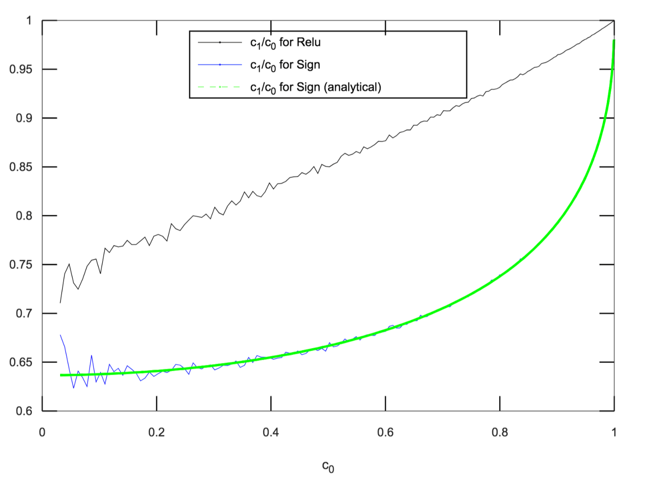
However, we are unable to account for the distribution around the expected value and prove that the magnitude of the expected value of the sum of $n$ such random variables drops exponentially with height. Hence, we leave this as a conjecture that we believe to be true.

As in the $\mathrm{sgn}$ case, SQ-hardness hardness for $\mathrm{relu}$ activation follows directly from the above conjecture, using Section 4.

Now take a subset of $k$ binary inputs $x$ so that no pair is equal to one another or opposite; that is, $x_{i}\neq\pm x_{j}$. We will also exclude opposites among the $k$ inputs.

References

- [1] A. Anandkumar and R. Ge. Efficient approaches for escaping higher order saddle points in non-convex optimization. In COLT, pages 81–102, 2016.
- [2] A. Brutzkus and A. Globerson. Globally optimal gradient descent for a convnet with Gaussian inputs. In ICML, pages 605–614, 2017.
- [3] N. H. Bshouty and V. Feldman. On using extended statistical queries to avoid membership queries. JMLR, 2:359–395, 2002.
- [4] A. Daniely. Complexity theoretic limitations on learning halfspaces. In PODS, pages 105–117, 2016.
- [5] I. Diakonikolas, D. M. Kane, and A. Stewart. Statistical query lower bounds for robust estimation of high-dimensional Gaussians and Gaussian mixtures. In FOCS, pages 73–84, 2017.
- [6] S. S. Du, J. D. Lee, and Y. Tian. When is a convolutional filter easy to learn? Preprint arXiv:1709.06129, 2017.
- [7] S. S. Du, J. D. Lee, Y. Tian, A. Singh, and B. Póczos. Gradient descent learns one-hidden-layer CNN: don’t be afraid of spurious local minima. In ICML, pages 1338–1347, 2018.
- [8] V. Feldman. A general characterization of the statistical query complexity. In COLT, pages 785–830, 2017.
- [9] S. Goel, V. Kanade, A. R. Klivans, and J. Thaler. Reliably learning the ReLU in polynomial time. In COLT, pages 1004–1042, 2017.
- [10] S. Goel and A. Klivans. Learning depth-three neural networks in polynomial time. Preprint arXiv:1709.06010, 2017.
- [11] S. Goel and A. R. Klivans. Eigenvalue decay implies polynomial-time learnability for neural networks. In NIPS, pages 2189–2199, 2017.
- [12] M. X. Goemans and D. P. Williamson. Improved approximation algorithms for maximum cut and satisfiability problems using semidefinite programming. J. ACM, 42(6):1115–1145, 1995.
- [13] M. Janzamin, H. Sedghi, and A. Anandkumar. Beating the perils of non-convexity: Guaranteed training of neural networks using tensor methods. Preprint arXiv:1506.08473, 2015.
- [14] M. J. Kearns. Efficient noise-tolerant learning from statistical queries. JACM, 45(6):983–1006, 1998.
- [15] A. R. Klivans and A. A. Sherstov. Cryptographic hardness for learning intersections of halfspaces. JCSS, 75(1):2–12, 2009.
- [16] Y. Li and Y. Yuan. Convergence analysis of two-layer neural networks with ReLU activation. In NIPS, pages 597–607, 2017.
- [17] E. Ng and M. Geller. A table of integrals of the error functions. Journal OF Research of the National Bureau of Standards, 73B(1), 1969.
- [18] R. Panigrahy, A. Rahimi, S. Sachdeva, and Q. Zhang. Convergence results for neural networks via electrodynamics. In ITCS, pages 22:1–22:19, 2018.
- [19] Y. Zhang, J. D. Lee, M. J. Wainwright, and M. I. Jordan. Learning halfspaces and neural networks with random initialization. Preprint arXiv:1511.07948, 2015.
- [20] K. Zhong, Z. Song, and I. S. Dhillon. Learning non-overlapping convolutional neural networks with multiple kernels. Preprint arXiv:1711.03440, 2017.
- [21] K. Zhong, Z. Song, P. Jain, P. L. Bartlett, and I. S. Dhillon. Recovery guarantees for one-hidden-layer neural networks. In ICML, pages 4140–4149, 2017.