New developments of the methodology of the Modified method of simplest equation with application

Nikolay K. Vitanov

Institute of Mechanics, Bulgarian Academy of Sciences, Akad. G. Bonchev Str., Bl. 4, 1113 Sofia, Bulgaria

Abstract

We discuss an extension of the modified method of simplest equation for obtaining exact analytical solutions of nonlinear partial differential equations. The extension includes the possibility for use of: (i) more than one simplest equation; (ii) relationship that contains as particular cases the relationship used by Hirota [1] and the relationship used in the previous version of the methodology; (iii) transformation of the solution that contains as particular case the possibility of use of the Painleve expansion; (iv) more than one balance equation. The discussed version of the methodology allows: obtaining multi-soliton solutions of nonlinear partial differential equations if such solutions do exist and obtaining particular solutions of nonintegrable nonlinear partial differential equations. Examples for the application of the methodology are discussed.

1 Introduction

Differential equations occur in the process of mathematical study of many problems from natural and social sciences as these equations relate quantities to their changes and such relationships are frequently encountered. Nonlinear differential equations are used for modeling of processes in many branches of science such as fluid mechanics, atmospheric and ocean sciences, mathematical biology, social dynamics, etc. [2] - [13]. In many cases the model equations are nonlinear partial differential equations and their exact solutions help us to understand complex nonlinear phenomena such as existence and change of different regimes of functioning of complex systems, spatial localization, etc. Because of the above the exact solutions of nonlinear partial differential equations are studied intensively [14] - [22]. In the yearly years of the research on the methodology for obtaining exact solutions of nonlinear partial differential equations one has searched for transformations that can transform the solved nonlinear partial differential equation to a linear differential equation. Numerous attempts for obtaining such transformations have been made and in 1967 Gardner, Green, Kruskal and Miura [17] managed to connect the Korteweg - de Vries equation to the inverse scattering problem for the linear Schödinger equation. This methodology is known today as Method of Inverse Scattering Transform, [14]. Below we are interested in another line of research that was followed by Hirota who developed a direct method for obtaining such exact solutions - Hirota method [1], [23]. Hirota method is based on bilinearization of the solved nonlinear partial differential equation by means of appropriate transformations. Truncated Painleve expansions may lead to many of these appropriate transformations [22], [24], [25] and the study of the applications of these truncated expansions [26] leaded to the formulation of the Method of Simplest Equation (MSE) [27], [28]. We refer to the articles of Kudryashov and co-authors for further results connected to MSE [29] - [37].

I have started my work on the method of simplest equation by proposing the use of the ordinary differential equation of Bernoulli as simplest equation [38] and by application of the method to ecology and population dynamics [39] where the concept of the balance equation has been used. Today the method of simplest equation has two versions. The original version of Kudryashov is called Method of Simplest Equation - MSE and there the determination of the truncation of the corresponding series of solutions of the simplest equation is based on the first step in the algorithm for detection of the Painleve property. An equivalent version is called Modified Method of Simplest Equation - MMSE or Modified Simple Equation Method - MSEM [28], [40], [41]. It if based on determination of the kind of the simplest equation and truncation of the series of solutions of the simplest equation by means of application of a balance equation. Up to now our contributions to the methodology and its application are connected to this version of the method [42] - [47] and in [48] where we have extended the methodology of the MMSE to simplest equations of the class

(1)

\left(\frac{d^{k}g}{d\xi^{k}}\right)^{l}=\sum\limits_{j=0}^{m}d_{j}g^{j}

where $k=1,\dots$ , $l=1,\dots$ , and $m$ and $d_{j}$ are parameters. The solution of Eq.(1) defines a special function that contains as particular cases, e.g.: trigonometric functions; hyperbolic functions; elliptic functions of Jacobi; elliptic function of Weierstrass. Our goal is to extend the methodology of MSE and MMSE in order to make it applicable to larger classes of nonlinear partial differential equations.

The text below is organized as follows. In Sect. 2 we discuss a version the modified method of simplest equation that makes the methodology capable to obtain multi-soliton solutions of nonlinear partial differential equations. Sect.3 contains examples of applications of the method. Several concluding remarks are given in Sect. 4.

2 Extended version of the modified method of simplest equation

In the previous version of the method we have used a representation of the searched solution of a nonlinear partial differential equation as power series of a solution of a simplest equation. This approach does not work for the case of search for bisoliton, trisoliton, and multisoliton solutions because the previous version of the modified method of simplest equation was connected to the use of a single simplest equation. If we allow for use of more than one simplest equation then the modified method of simplest equation can be formulated in a way that makes obtaining of multisoliton solutions possible. Below we formulate such a version of the modified method of simplest equation. The schema of the old and the new version of the methodology is shown in Fig. 1.

Refer to caption — Figure 1: Schema of the previous version (righ-hand side) and of the extended version (left-hand side) of the Modified method of simplest equation. The transformation used in the extended version of the method contains as particular case the transformation used in the previous version of the method. The form of the function $F$ used in the extended version of the method contains as particular case the form of the function used in the previous version of the method. The new form of the function $F$ contains as particular case also the form of the function used by Hirota. In the extended form of the method more than one simplest equation can be used and more than one balance equation can arise. In the previous version of the method one uses one simplest equation and one balance equation.

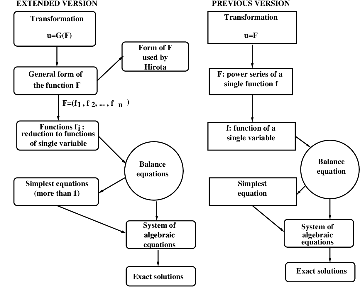
Let us consider a nonlinear partial differential equation

(2)

{\cal{R}}(u,\dots)=0

where ${\cal{R}}(u,\dots)$ depends on the function $u(x,...,t)$ and some of its derivatives participate in ( $u$ can be a function of more than 1 spatial coordinate). The 7 steps of the extended modified method of simplest equation are as follows.
Step 1.) We apply a transformation

(3)

u(x,\dots,t)=H(F(x,\dots,t))

where $H(F)$ is some function of another function $F$ . In general $F(x,\dots,t)$ is a function of the spatial variables as well as of the time. The transformation $H(F)$ may be the Painleve expansion [1], [19], [26], [49], [50] or another transformation, e.g., $u(x,t)=4\tan^{-1}[F(x,t)]$ for the case of the sine - Gordon equation, etc. [51] - [55]. In many particular cases one may skip this step (then we have just $u(x,\dots,t)=H(x,\dots,t)$ ) but in some cases the step is necessary for obtaining a solution of the studied nonlinear PDE. The application of Eq.(3) to Eq.(2) leads to a nonlinear PDE for the function $F(x,\dots,t)$ .
Step 2.) The function $F(x,\dots,t)$ is represented as a function of other functions $f_{1},\dots,f_{N}$ ( $N=1,2,\dots$ ) that are connected to solutions of some differential equations (these equations can be partial or ordinary differential equations) that are more simple than Eq.(2). We stress that the forms of the function $F(f_{1},\dots,f_{N})$ can be different. One example is

(4)		$\displaystyle F$	$\displaystyle=$	$\displaystyle\alpha+\sum\limits_{i_{1}=1}^{N}\beta_{i_{1}}f_{i_{1}}+\sum\limits_{i_{1}=1}^{N}\sum\limits_{i_{2}=1}^{N}\gamma_{i_{1},i_{2}}f_{i_{1}}f_{i_{2}}+\dots+$
(4)				$\displaystyle\sum\limits_{i_{1}=1}^{N}\dots\sum\limits_{i_{N}=1}^{N}\sigma_{i_{1},\dots,i_{N}}f_{i_{1}}\dots f_{i_{N}}$

where $\alpha,\beta_{i_{1}},\gamma_{i_{1},i_{2}},\sigma_{i_{1},\dots,i_{N}}\dots$ are parameters. The relationship (4) contains as particular case the relationship used by Hirota [1]. The power series $\sum\limits_{i=0}^{N}\mu_{n}f^{n}$ (where $\mu$ is a parameter) used in the previous versions of the methodology of the modified method of simplest equation are a particular case of the relationship (4) too.
Step 3.) In general the functions $f_{1},\dots,f_{N}$ are solutions of partial differential equations. By means of appropriate ansätze (e.g., traveling-wave ansätze such as $\xi=\hat{\alpha}x+\hat{\beta}t$ ; $\zeta=\hat{\gamma}x+\hat{\delta}t$ , $\eta=\hat{\mu}y+\hat{\nu}t\dots$ ) the solved differential equations for $f_{1},\dots,f_{N}$ may be reduced to differential equations $D_{l}$ , containing derivatives of one or several functions

(5)

D_{l}\left[a(\xi),a_{\xi},a_{\xi\xi},\dots,b(\zeta),b_{\zeta},b_{\zeta\zeta},\dots\right]=0;\ \ l=1,\dots,N

If the equations for the functions $f_{1},\dots$ are ordinary differential equations one may skip this step but the step may be necessary if the equations for $f_{1},\dots$ are partial differential equations.
Step 4.) We assume that the functions $a(\xi)$ , $b(\zeta)$ , etc., are functions of other functions, e.g., $v(\xi)$ , $w(\zeta)$ , etc., i.e.

(6)

a(\xi)=A[v(\xi)];\ \ b(\zeta)=B[w(\zeta)];\dots

We note that the functions $A$ , $B$ , $\dots$ are not prescribed. One may use a finite-series relationship, e.g.,

(7)

a(\xi)=\sum_{\mu_{1}=-\nu_{1}}^{\nu_{2}}q_{\mu_{1}}[v(\xi)]^{\mu_{1}};\ \ \ b(\zeta)=\sum_{\mu_{2}=-\nu_{3}}^{\nu_{4}}r_{\mu_{2}}[w(\zeta)]^{\mu_{2}},\dots

(where $q_{\mu_{1}}$ , $r_{\mu_{2}}$ , $\dots$ are coefficients) but other kinds of relationships may be used too.
Step 5.) The functions $v(\xi)$ , $w(\zeta)$ , $\dots$ are solutions of simpler ordinary differential equations called simplest equations, i.e., the extended version of the methodology allows for the use of more than one simplest equation.
Step 6.) The application of the steps 1.) - 5.) to Eq.(2) transforms the left-hand side of this equation. Let the result of this transformation be a function that is a sum of terms where each term contains some function multiplied by a coefficient. This coefficient contains some of the parameters of the solved equation and some of the parameters of the solution. In the most cases a balance procedure must be applied in order to ensure that the above-mentioned relationships for the coefficients contain more than one term. This balance procedure may lead to one or more additional relationships balance equations among the parameters of the solved equation and parameters of the solution.
Step 7.) We may obtain a nontrivial solution of Eq. (2) if all coefficients mentioned in Step 6.) are set to $0$ . This condition usually leads to a system of nonlinear algebraic equations for the coefficients of the solved nonlinear PDE and for the coefficients of the solution. Any nontrivial solution of the above algebraic system leads to a solution the studied nonlinear partial differential equation.

3 Examples

3.1 The most simple example: bisoliton solution of the Korteweg-de Vries equation

We shall describe this example very briefly in order to show the capacity of the extended version of the methodology to lead to multi - soliton solutions of integrable partial differential equations. We consider a version of the Korteweg - de Vries equation

(8)

u_{t}+\sigma uu_{x}+u_{xxx}=0

where $\sigma$ is a parameter. The 7 steps of the application of the version of the modified method of simplest equation from Sect. 2 are as follows.
Step 1.) The transformation
We set $u=p_{x}$ in Eq.(8). The result is integrated and we apply the transformation $p=\frac{12}{\sigma}(\ln F)_{x}$ . The result is

(9)

FF_{tx}+FF_{xxxx}-F_{t}F_{x}+3F_{xx}^{2}-4F_{x}F_{xxx}=0

Step 2.) Relationship among $F(x,t)$ and two functions $f_{1,2}$ that will be connected below to two simplest equations
We shall use two functions $f_{1}(x,t)$ and $f_{2}(x,t)$ and the relationship for $F$ is assumed to be a particular case of Eq.(4):

(10)

F(x,t)=1+f_{1}(x,t)+f_{2}(x,t)+cf_{1}(x,t)f_{2}(x,t)

where $c$ is a parameter. The substitution of Eq.(10) in Eq.(9) leads to a nonlinear partial differential equation containing 64 terms.
Step 3.) Equations for the functions $f_{1}(x,t)$ and $f_{2}(x,t)$
The structure of the obtained allow us to assume a the simple form of the equations for the functions $f_{1,2}$ :

(11)

\displaystyle\frac{\partial f_{1}}{\partial x}=\alpha_{1}f_{1};\ \ \ \frac{\partial f_{1}}{\partial t}=\beta_{1}f_{1};\frac{\partial f_{2}}{\partial x}=\alpha_{2}f_{2};\ \ \ \frac{\partial f_{2}}{\partial t}=\beta_{2}f_{2};

Eq.(11) transforms the solved nonlinear partial differential equation to a polynomial of $f_{1}$ and $f_{2}$ . Further we assume that $\xi=\alpha_{1}x+\beta_{1}t+\gamma_{1}$ and $\zeta=\alpha_{2}x+\beta_{2}t+\gamma_{2}$ and $f_{1}(x,t)=a(\xi);\ \ \ f_{2}(x,t)=b(\zeta)$ where $\alpha_{1,2}$ , $\beta_{1,2}$ and $\gamma_{1,2}$ are parameters.
Step 4.) Relationships connecting $a(\xi)$ and $b(\zeta)$ to the functions $v(\xi)$ and $w(\zeta)$ that are solutions of the simplest equations
In the discussed here case the relationships are quite simple. We can use Eq.(16) for the cases $\mu_{1}=\nu_{2}=1$ and $\mu_{2}=\nu_{4}=1$ . The result is: $a(\xi)=q_{1}v(\xi);\ \ \ b(\zeta)=r_{1}w(\zeta)$ .
Step 5.) Simplest equations for $v(\xi)$ and $w(\zeta)$
The simplest equations are

(12)

\frac{dv}{d\xi}=v;\ \ \ \frac{dw}{d\zeta}=w

and the corresponding solutions are $v(\xi)=\omega_{1}\exp(\xi);\ \ \ w(\zeta)=\omega_{2}\exp(\zeta)$ . Below we shall omit the parameters $\omega_{1,2}$ as they can be included in the parameters $q_{1}$ and $r_{1}$ respectively. We shall omit also $q_{1}$ and $r_{1}$ as they can be included in $\xi$ and $\zeta$ .
Step 6.) Transformation of the nonlinear PDE that contains 64 terms
The substitution of all above in the nonlinear partial differential equation that contains 64 terms leads to a sum of exponential functions and each exponential function is multiplied by a coefficient. Each of these coefficients is a relationship containing the parameters of the solution and all of the relationships contain more than one term. Thus we don’t need to perform a balance procedure.
Step 7.) Obtaining and solving the system of algebraic equations
The system of algebraic equations is obtained by setting of above-mentioned relationships to $0$ . Thus we obtain the following system:

	$\displaystyle\alpha_{1}^{3}+\beta_{1}=0,\ \ \ \alpha_{2}^{3}+\beta_{2}=0,$
	$\displaystyle(c+1)\alpha_{1}^{4}+4\alpha_{2}(c-1)\alpha_{1}^{3}+6\alpha_{2}^{2}(c+1)\alpha_{1}^{2}+[(4c-4)\alpha_{2}^{3}+(\beta_{1}+\beta_{2})c+$
(13)		$\displaystyle\beta_{1}-\beta_{2}]\alpha_{1}+[(c+1)\alpha_{2}^{3}+(\beta_{1}+\beta_{2})c-\beta_{1}+\beta_{2}]\alpha_{2}=0.$

The non-trivial solution of this system is: $\beta_{1}=-\alpha_{1}^{3};\ \ \beta_{2}=-\alpha_{2}^{3};\ \ c=\frac{(\alpha_{1}-\alpha_{2})^{2}}{(\alpha_{1}+\alpha_{2})^{2}}$ and the corresponding solution of Eq.(8) is

(14)		$\displaystyle u(x,t)$	$\displaystyle=$	$\displaystyle\frac{12}{\sigma}\frac{\partial^{2}}{\partial x^{2}}\Bigg[1+\exp\Big(\alpha_{1}x-\alpha_{1}^{3}t+\gamma_{1}\Big)+\exp\Big(\alpha_{2}x-\alpha_{2}^{3}t+\gamma_{2}\Big)+$
(14)				$\displaystyle\frac{(\alpha_{1}-\alpha_{2})^{2}}{(\alpha_{1}+\alpha_{2})^{2}}\exp\Big((\alpha_{1}+\alpha_{2})x-(\alpha_{1}^{3}+\alpha_{2}^{3})t+\gamma_{1}+\gamma_{2}\Big)\Bigg]$

Eq.(14) describes the bisoliton solution of the Korteweg - de Vries equation.

3.2 Second example: the generalized Maxwell-Cataneo equation

As a second example we shall consider a nonlinear partial differential equation that is a generalization of the Maxwell-Cataneo kind of equation

(15)

u_{t}+ru^{a}u_{tt}=pu^{b-1}u_{x}^{2}+qu^{b}u_{xx}

The original Maxwell-Cataneo kind of equation is obtained when $a=0$ , $b=1$ [56]. We follow the methodology for the case $u(x,t)=H[F(x,t)]=F(x,t)$ . and search for traveling waves by using the traveling-wave ansatz $F(x,t)=F(\xi)=F(\alpha x+\beta t)$ that reduces the solved nonlinear PDE to a nonlinear ODE. Then the solution $F(\xi)$ is searched as some function of another function $f(\xi)$ , i.e.,

(16)

F(\xi)=\sum_{\mu=-\nu}^{\nu_{1}}p_{\mu}[f(\xi)]^{\mu},

$p_{\mu}$ are coefficients and $f(\xi)$ is a solution of simpler ordinary differential equation (the simplest equation):

(17)

f_{\xi}=n\left[f^{(n-1)/n}-f^{(n+1)/n}\right],

where $n$ is an appropriate positive real number. The solution of this equation is $f(\xi)=\tanh^{n}(\xi)$ . $n$ must be such real number that $\tanh^{n}(\xi)$ exists for $\xi\in(-\infty,+\infty)$ ( $n=1/5$ is an appropriate value for $n$ and $n=1/4$ is not an appropriate value for $n$ ). Following the steps of the methodology we obtain two balance equations: $a=b=\frac{1}{n}$ , and the nonlinear partial differential equation (15) is reduced to the system of nonlinear algebraic equations

	$\displaystyle r(n+1)\beta^{2}-[(p+q)n+q]\alpha^{2}=0$
	$\displaystyle\Bigg\{r(n-1)\beta^{2}-\Bigg[\Bigg((p+q)n-q\Bigg)\Bigg]\alpha^{2}\Bigg\}\delta^{1/n}+\beta=0$
(18)		$\displaystyle\Bigg[(p+q)\alpha^{2}-r\beta^{2}\Bigg]n\delta^{1/n}-\frac{1}{2}\beta=0.$

One non-trivial solution of this system is

(19)

\alpha=\frac{1}{2npr^{1/2}\delta^{1/n}}\Bigg[(n+1)(np+nq+q)\Bigg]^{1/2};\ \ \beta=\frac{np+nq+q}{2npr\delta^{1/n}},

and the corresponding solution of Eq.(15) is

\displaystyle u(x,t)=\delta\tanh^{n}\Bigg\{\frac{1}{2npr^{1/2}\delta^{1/n}}\Bigg[\Bigg((n+1)(np+nq+q)\Bigg)^{1/2}x+\frac{np+nq+q}{r^{1/2}}t\Bigg]\Bigg\}.

Several particular cases are as follows. For $n=1$ : the equation

(21)

u_{t}+ruu_{tt}=pu_{x}^{2}+quu_{xx},

has the solution

(22)

u(x,t)=\delta\tanh\Bigg\{\frac{1}{2pr^{1/2}\delta}\Bigg[\Bigg(2(p+2q)\Bigg)^{1/2}x+\frac{p+2q}{r^{1/2}}t\Bigg]\Bigg\}.

For $n=2$ : the equation

(23)

u_{t}+ru^{1/2}u_{tt}=pu^{-1/2}u_{x}^{2}+qu^{1/2}u_{xx},

has the solution

(24)

u(x,t)=\delta\tanh^{2}\Bigg\{\frac{1}{4pr^{1/2}\delta^{1/2}}\Bigg[\Bigg(3(2p+3q)\Bigg)^{1/2}x+\frac{2p+3q}{r^{1/2}}t\Bigg]\Bigg\}.

Finally let $n=1/3$ . Then the equation

(25)

u_{t}+ru^{3}u_{tt}=pu^{2}u_{x}^{2}+qu^{3}u_{xx},

has the solution

(26)

u(x,t)=\delta\tanh^{1/3}\Bigg\{\frac{3}{2pr^{1/2}\delta^{3}}\Bigg[\Bigg(\frac{4}{9}(p+4q)\Bigg)^{1/2}x+\frac{p+4q}{3r^{1/2}}t\Bigg]\Bigg\}.

4 Concluding remarks

Above we have discussed an extended version of the methodology of the modified method of simplest equation. The extension is based on the possibility of use of more than one simplest equation, on a transformation connected to the searched solution and on a possibility of use of more general relationship among the solution of the solved nonlinear partial differential equation and the solutions of the simplest equations. These possibilities add the capability for obtaining multisolitons to the discussed extended methodology by keeping its ability to lead to particular exact solutions of nonintegrable nonlinear partial differential equations. Two examples of application of the methodology are presented and it is demonstrated that the balance procedure can lead to ore than one balance equation.

References

[1] R. Hirota. Exact solution of Korteweg-de Vries equation for multiple collisions of solitons. Phys. Rev. Lett., 27 (1971) 1192 – 1194.
[2] L. Debnath. Nonlinear partial differential equations for scientists and engineers. Springer, New York, 2012.
[3] J. D. Murray, Lectures on nonlinear differential equation models in biology. Oxford University Press, Oxford, UK 1977.
[4] F. Verhulst. Nonlinear differential equations and dynamical systems. Springer, Berlin, 1990.
[5] N. K. Vitanov, N. Martinov. On the solitary waves in the sine-Gordon model of the two-dimensional Josephson junction. Zeitschrift fuer Physik B 100, (1996), 129 – 135.
[6] N. K. Vitanov, F. H. Busse. Bounds on the heat transport in a horizontal fluid layer with stress-free boundaries. Zeitschrift für Angewandte Mathematik und Physik ZAMP, 48, (1997) 310 – 324.
[7] N. K. Vitanov. Upper bounds on the heat transport in a porous layer. Physica D, 136, (2000) 322 – 339.
[8] Z. I. Dimitrova, N. K. Vitanov. Influence of adaptation on the nonlinear dynamics of a system of competing populations. Physics Letters A, 272, (2000), 368 – 380.
[9] Z. I. Dimitrova, N. K. Vitanov. Chaotic pairwise competition. Theoretical Population Biology, 66, (2004) 1 – 12.
[10] S. Panchev, T. Spassova, N. K. Vitanov. Analytical and numerical investigation of two families of Lorenz-like dynamical systems. Chaos, Solitons & Fractals, 33, 1658 - 1671 (2007).
[11] N. K. Vitanov, I. P. Jordanov, Z. I. Dimitrova. On nonlinear dynamics of interacting populations: Coupled kink waves in a system of two populations. Communication in Nonlinear Science and Numerical Simulation, 14, (2009), 2379 – 2388.
[12] N. K. Vitanov, I. P. Jordanov, Z. I. Dimitrova. On nonlinear population waves. textitApplied Mathematics and Computation, 215, (2009), 2950 – 2964.
[13] N. K. Vitanov. Science dynamics and research production. Indicators, indexes, statistical laws and mathematical models. Springer, Cham, 2016.
[14] M. J. Ablowitz, P. A. Clarkson. Solitons, nonlinear evolution equations and inverse scattering. Cambridge University Press, Cambridge, 1991.
[15] W. F. Ames. Nonlinear partial differential equations in engineering. Academic Press, New York, 1972.
[16] A. Benkirane, J. -P. Gossez (Eds.) Nonlinear partial differential equations. Addison Wesley Longman, Essex, UK, 1996.
[17] C. S. Gardner, J. M. Greene, M. D. Kruskal, R. R. Miura. Method for solving Korteweg-de Vries equation. Phys. Rev. Lett., 19 (1967) 1095 – 1097.
[18] P. Holmes, J. L. Lumley, G. Berkooz. Turbulence, coherent structures, dynamical systems and symmetry. Cambridge University Press, Cambridge, 1996.
[19] N. A. Kudryashov. Exact solutions of the generalized Kuramoto - Sivashinsky equation. Phys. Lett. A, 147, (1990) 287 – 291.
[20] J. D. Logan. An introduction to nonlinear partial differential equations. Wiley, New York, 2008.
[21] M. Remoissenet. Waves called solitons. Springer, Berlin, 1993.
[22] M. Tabor. Chaos and integrability in dynamical systems. Wiley, New York, 1989.
[23] R. Hirota. The direct method in soliton theory. Cambridge University Press, Cambridge, 2004.
[24] F. Carrielo, M. Tabor. Painleve expansions for nonlinear nonitegrable evolution equations. Physica D, 39, (1989) 77 – 94.
[25] J. Weiss, M. Tabor, G. Carnevalle. The Painleve property for partial differential equations. Journal of Mathematical Physics, 24, (1983) 522 – 526.
[26] N. K. Kudryashov. On types of nonlinear nonitegrable equations with exact solutions. Physics Letters A, 155, (1991) 269 – 275.
[27] N. A. Kudryshov. Simplest equation method to look for exact solutions of nonlinear differential equations. Chaos, Solitons & Fractals, 24, (2005) 1217 – 1231.
[28] N. A. Kudryashov, N. B. Loguinova. Extended simplest equation method for nonlinear differential equations. Applied Mathematics and Computation, 205, (2008) 361 – 365.
[29] N. A. Kudryashov, M. V. Demina. Polygons of differential equations for finding exacts solutions. Chaos, Solitons & Fractals, 33, (2007) 1480 – 1496.
[30] M. V. Demina, N. A. Kudryashov, D. I. Sinelshchikov. The polygonal method for constructing exact solutions to certain nonlinear differential equations describing water waves. Computational Mathematics and Mathematical Physics, 48, (2008) 2182 – 2193.
[31] N. A. Kudryashov, M. V. Demina. Traveling wave solutions of the generalized nonlinear evolution equations. Applied Mathematics and Computation, 201, (2009) 551 – 557.
[32] N. A. Kudryashov. Exact solutions of the Swift-Hohenberg equation with dispersion. Communications in Nonlinear Science and Numerical Simulation, 17 (2012) 26 – 34.
[33] N. A. Kudryashov, D. I. Sinelshchikov. Elliptic solutions for a family of fifth order nonlinear evolution equations. Applied Mathematics and Computation, 218, (2012) 6991 – 6997.
[34] N. A. Kudryashov. One method for finding exact solutions of nonlinear differential equations. Communications in Nonlinear Science and Numerical Simulation, 17, (2012) 2248 – 2253.
[35] N. A. Kudryashov, D. I. Sinelshchikov. Nonlinear differential equations of the second, third and fourth order with exact solutions. Applied Mathematics and Computation, 218, (2012) 10454 – 10467.
[36] N. A. Kudryashov, M. B. Soukharev, M. V. Demina. Elliptic traveling waves of the Olver equation. Communications in Nonlinear Science and Numerical Simulation, 17, (2012) 4104 – 4114.
[37] N. A. Kudryashov. Polynomials in logistic functions and solitary waves of nonlinear differential equations. Applied Mathematics ans Computation, 219, (2013) 9245 – 9253.
[38] N. K. Vitanov. Application of simplest equations of Bernoulli and Riccati kind for obtaining exact traveling-wave solutions for a class of PDEs with polynomial nonlinearity. Communications in Nonlinear Science and Numerical Simulation, 15, (2010) 2050 – 2060.
[39] N. K. Vitanov, Z. I. Dimitrova. Application of the method of simplest equation for obtaining exact traveling-wave solutions for two classes of model PDEs from ecology and population dynamics. Communications in Nonlinear Science and Numerical Simulation, 15, (2010) 2836 – 2845.
[40] N. K. Vitanov, Z. I. Dimitrova, H. Kantz. Modified method of simplest equation and its application to nonlinear PDEs. Applied Mathematics and Computation, 216, (2010) 2587 – 2595.
[41] N. K. Vitanov. Modified method of simplest equation: powerful tool for obtaining exact and approximate traveling-wave solutions of nonlinear PDEs. Communications in Nonlinear Science and Numerical Simulation, 16, (2011) 1176 – 1185.
[42] N. K. Vitanov, Z. I. Dimitrova, K. N. Vitanov. On the class of nonlinear PDEs that can be treated by the modified method of simplest equation. Application to generalized Degasperis–Processi equation and b-equation. Communications in Nonlinear Science and Numerical Simulation, 16, (2011) 3033 – 3044.
[43] N. K. Vitanov. On modified method of simplest equation for obtaining exact and approximate solutions of nonlinear PDEs: the role of the simplest equation. Communications in Nonlinear Science and Numerical Simulation, 16, (2011) 4215 – 4231.
[44] N. K. Vitanov, Z. I. Dimitrova, H. Kantz. Application of the method of simplest equation for obtaining exact traveling-wave solutions for the extended Korteweg - de Vries equation and generalized Camassa - Holm equation. Applied Mathematics and Computation, 219, (2013) 7480 – 7492.
[45] N. K. Vitanov, Z. I. Dimitrova, K. N. Vitanov. Traveling waves and statistical distributions connected to systems of interacting populations. Computers & Mathematics with Applications, 66, (2013) 1666 – 1684.
[46] N. K. Vitanov, Z. I. Dimitrova. Solitary wave solutions for nonlinear partial differential equations that contain monomials of odd and even grades with respect to participating derivatives. Applied Mathematics and Computation, 247, (2014) 213 – 217.
[47] N. K. Vitanov, Z. I. Dimitrova, T. I. Ivanova. On solitary wave solutions of a class of nonlinear partial differential equations based on the function $1/cosh^{n}(\alpha x+\beta t)$ . Applied Mathematics and Computation, 315, (2017) 372 – 380.
[48] N. K. Vitanov, Z. I. Dimitrova, K. N. Vitanov. Modified method of simplest equation for obtaining exact analytical solutions of nonlinear partial differential equations: Further development of the methodology with applications. Applied Mathematics and Computation, 269, (2015) 363 – 378.
[49] J. Weiss. The Painleve property for partial differential equations. Bäcklund transformations, Lax pair, and the Schwarzian derivative. Journal of Mathematical Physics, 24, (1983) 1405 – 1413.
[50] N. A. Kudryashov. Soliton, rational and special solutions of the Korteweg - de Vries hierarchy. Applied Mathematics and Computation, 217, (2010) 1774 – 1779.
[51] N. Martinov, N. Vitanov. On the correspondence between the self-consistent 2D Poisson-Boltzmann structures and the sine-Gordon waves. Journal of Physics A: Mathematical and General, 25, (1992) L51 – L56.
[52] N. Martinov, N. Vitanov. On some solutions of the two-dimensional sine-Gordon equation. Journal of Physics A: Mathematical and General, 25, (1992) L419 – L426.
[53] N. K. Martinov, N. K. Vitanov. New class of running-wave solutions of the (2+1)-dimensional sine-Gordon equation. Journal of Physics A: Mathematical and General, 27, (1994) 4611 - 4618.
[54] N. K. Martinov, N. K. Vitanov. On the self-consistent thermal equilibrium structures in two-dimensional negative-temperature systems. Canadian Journal of Physics, 72, (1994) 618 – 624.
[55] N. K. Vitanov. On travelling waves and double-periodic structures in two-dimensional sine-Gordon systems. Journal of Physics A: Mathematical and General, 29, (1996) 5195 – 5207.
[56] A. P. Reverberi, P. Bagnerini, L. Maga, A. G. Bruzzone. On the nonlinear Maxwell-Cataneo equation with non-constant diffusivity: Shock and discontinuity waves. International Journal of Heat and Mass Transfer, 51, (2008) 5327 – 5332.