Baryon acoustic oscillations at from the correlations of Ly absorption in eBOSS DR14
Abstract
We measure the imprint of primordial baryon acoustic oscillations (BAO) in the correlation function of Ly absorption in quasar spectra from the Baryon Oscillation Spectroscopic Survey (BOSS) and the extended BOSS (eBOSS) in Data Release 14 (DR14) of the Sloan Digital Sky Survey (SDSS)-IV. In addition to 179,965 spectra with absorption in the Lyman- (Ly) region, we use, for the first time, Ly absorption in the Lyman- region of 56,154 spectra. We measure the Hubble distance, , and the comoving angular diameter distance, , relative to the sound horizon at the drag epoch at an effective redshift . Using a physical model of the correlation function outside the BAO peak, we find and , within 1 from the flat-CDM model consistent with CMB anisotropy measurements. With the addition of polynomial “broadband” terms, the results remain within one standard deviation of the CMB-inspired model. Combined with the quasar-Ly cross-correlation measurement presented in a companion paper (Blomqvist et al. 2019), the BAO measurements at are within 1.7 of the predictions of this model.
Key Words.
cosmological parameters - dark energy - cosmology : observations1 Introduction
Since the first observations of the imprint of primordial baryonic acoustic oscillations (BAO) as a peak in the galaxy correlation function (Eisenstein et al. 2005) or as a periodic modulation in the corresponding power spectrum (Cole et al. 2005), the BAO signal has led to significant constraints on cosmological parameters. The BAO peak in the radial direction at a redshift yields , where is the Hubble parameter and is the sound horizon at the drag epoch (Eisenstein & Hu 1998). The transverse measurement constrains the quantity , where is the angular diameter distance. Because of its sensitivity to both the distance and the expansion rate, the ensemble of BAO measurements yield tight constraints on CDM parameters (Aubourg et al. 2015) even without the use of Cosmic Microwave Background (CMB) data.

Most BAO measurements have employed discrete objects like galaxies (Percival et al. 2010; Reid et al. 2010; Beutler et al. 2011; Blake et al. 2011; Anderson et al. 2012; Anderson et al. 2014a; Anderson et al. 2014b; Ross et al. 2015; Alam et al. 2017; Bautista et al. 2018) or quasars (Ata et al. 2018; Gil-Marín et al. 2018; Hou et al. 2018; Zarrouk et al. 2018). An alternative tracer of the density is the intergalactic medium (IGM), itself traced by Lyabsorption in quasar spectra. Such measurements at were suggested by McDonald 2003 and McDonald & Eisenstein 2007. The first detections of a BAO peak in the Ly auto-correlation function (Busca et al. 2013; Slosar et al. 2013) used data from the Baryon Oscillation Spectroscopic Survey (BOSS) in the Sloan Digital Sky Survey (SDSS) data-release 9 (DR9), at an effective redshift of . Delubac et al. 2015, using BOSS in SDSS-DR11, confirmed the detection of a BAO acoustic peak in the Ly auto-correlation function at the 5 level. Most recently, Bautista et al. 2017 (B17 hereafter) used Ly forests from BOSS DR12 data and provided a measurement of at 3.4% precision level (or of the optimal combination at the 2.5% level). The results were within 1 of the prediction of the flat CDM model favored by CMB anisotropies (Planck Collaboration et al. 2016). However, when combined with the BAO imprint on the cross-correlation of the Ly forest with BOSS DR12 quasars (du Mas des Bourboux et al. 2017), the values of and at differ by from this model. This mild tension was already present in the combined constraints of the cross-correlation measurement of Font-Ribera et al. 2014 and the auto-correlation of Delubac et al. 2015.
In the present paper, we use quasar spectra from the BOSS survey and from its extended version eBOSS in the SDSS DR14 to study BAO in the Lyauto-correlation function. The quasar-Lycross-correlation is studied in a companion paper (Blomqvist et al. 2019) As in previous measurements, we use Lyabsorption in the “Lyregion” of quasar spectra, i.e., quasar rest-frame wavelengths in the range nm. We call the auto-correlation function using only this region the Ly(Ly) Ly(Ly) correlation11 1 We use the notation “absorption(spectral region)” to distinguish the nature of absorption from the wavelength interval where the absorption is observed. Hence, the notation Ly(Ly) Ly(Ly) denotes Ly absorption in Ly regions correlated with Ly absorption in Ly regions. . To increase the statistical power we also include Ly absorption in the Ly regions of quasars, nm, correlated with the Ly absorption in Ly regions, i.e., the Ly(Ly)xLy(Ly) correlation function. The Ly region was previously used by Iršič et al. 2013 to investigate the flux transmission power spectrum within individual spectra.
Besides the use of the Lyregion, the analysis presented here differs in several ways from that of Bautista et al. 2017 based on DR12 data. For each quasar, we now use all observations instead of just the best one. We analyze % more Ly regions. We have refined the modelling of the weights (§3.2), the way we take into account the effect of unmasked High Column Density (HCD) systems, and the modeling of nonlinearities in the power spectrum (§4.1). We have not developed new mock spectra beyond those used in the DR12 analysis though this is being done for the final eBOSS analysis.
The layout of the paper is the following. In §2, we present the Ly and Ly spectral region samples used in the present study. We compute correlation function of Lyabsorption for the DR14 data in §3 and present our physical model for this function in §4. The results of fitting the data are presented and discussed in §5. We draw cosmological conclusions in §6 and summarize our results in §7.
The computations of the correlation functions presented in this paper have been performed using a dedicated software package, Package for Igm Cosmological-Correlations Analyses (picca), developed by our team22 2 Available at https://github.com/igmhub/picca..
2 Data sample and reduction


The extended Baryon Oscillation Spectroscopic Survey (eBOSS; Dawson et al. 2016) is the extension of the BOSS experiment (Dawson et al. 2013) which aims to measure cosmology with BAO using optical spectra from quasars, emission line galaxies and luminous red galaxies. It is one of the four projects of the fourth stage of the Sloan Digital Sky Survey (SDSS-IV; Blanton et al. 2017).
The optical spectra are collected from 1000 fibers, attached to the
focal plane of a 2.5 m telescope in Apache Point Observatory (Gunn et al. 2006), by two spectrographs in the wavelength range nm (Smee et al. 2013). The spectral resolution of the spectrographs is .
In this paper, we use the forests of the high-redshift quasar sample from the SDSS Data Release 14 (DR14; Abolfathi et al. 2017). This sample contains the first two years of eBOSS data and the five years of BOSS observations reprocessed using the eBOSS pipeline. It also includes data from the ancillary programs Time-Domain Spectroscopic Survey (TDSS) and SPectroscopic IDentification of ERosita Sources (SPIDERS). The quasar target selection is presented in Myers et al. 2015. Note that eBOSS also targets quasars at low redshifts (where the Ly region is not observable) to be used in other programs (Ata et al. 2018; Wang et al. 2018; Blomqvist et al. 2018; Zhao et al. 2019; du Mas des Bourboux et al. 2019).
The automated data reduction is organized in two steps (Dawson et al. 2016). The pipeline initially extracts the two-dimensional raw data into a one-dimensional
flux-calibrated spectrum. During this procedure, the spectra are wavelength and flux calibrated and the individual exposures of one object are coadded into a rebinned spectrum with .
The spectra are then classified as STAR or GALAXY or QSO, and their redshift is estimated.
Objects that cannot be automatically classified are visually inspected (Pâris et al. 2017) and a quasar catalog is produced, which contains 526,356 quasar spectra with redshift . Among these objects, 144,046 were not in DR12. The coverage footprint of DR14 quasars is presented in Fig.1
| Regions | forests | |||
|---|---|---|---|---|
| Ly | [97.4,102] | [360,459] | [2.53,3.5] | 56,154 |
| Ly | [104,120] | [360,540] | [2.0,3.5] | 179,965 |
In this study, we examine both Lyand Lyregions (see Fig. 2). The Lyregion in the quasar spectrum lies between the Lyand the Lyemission peaks. We limit its coverage to the rest-frame wavelength range [104,120] nm in order not to include the emission peaks, whose shape depends on the environment of the quasar. This approach minimizes the variance of the flux-transmission field defined in section 3.1. Similarly, we define the Lyregion as the rest-frame wavelength range [97.4,102] nm (Table 1, Fig. 2).
In the DR14 quasar catalog, selecting quasar redshifts in the range [2.0, 3.5] yields to 216,162 spectra containing, at least partially, the Lyregion, and selecting quasar redshifts in the range yields 86,245 spectra containing the Lyregion. We choose as an upper limit, as beyond this redshift the quasar density is insufficient to measure correlations and the rate of redshift misidentification is large (Busca & Balland 2018). The requirement that the observed wavelength must be greater than 360 nm is due to the low CCD response and atmospheric transmission in the UV region.
In order to mask damped Lysystems (DLA), we use the updated DR14 DLA catalog of Noterdaeme et al. 2009; Noterdaeme et al. 2012, which contains 34,541 DLA in 27,212 forests. The absorption of the identified DLAs are modeled with a Voigt profile and the regions with more than 20% of absorbed flux are masked. For the Lyregions, we apply this procedure both for Lyand Lystrong absorbers. We also mask the sky emission and absorption lines listed on the SDSS website33 3 http://classic.sdss.org/dr6/algorithms/linestable.html. The Broad Absorption Line (BAL) quasars are automatically identified (Pâris et al. 2017) and excluded from the data, leaving a sample of 201,286 objects for the Ly regions and 80,443 for the Ly regions.
For the determination of the correlation function, we divide spectra into “analysis pixels” that are the inverse-variance-weighted flux average over three adjacent pipeline pixels. Throughout the rest of this paper, “pixel” refers to analysis pixels unless otherwise stated. Spectral regions with less than 50 such pixels in regions or which have failed the continuum-fitting procedure (Sec. 3.1) are discarded. These selection criteria produce 179,965 Ly regions (compared to 157,783 in B17) and 56,154 Ly regions (see Table 1).
The analysis procedure described in the next section assigns redshifts to the observed pixel wavelengths by assuming that flux decrements, in both the Lyand Lyregions, are due to Lyabsorption. The effect of non-Lyabsorption is taken into account in the correlation-function model presented in §4. The weighted distribution of the redshifts of pairs of pixels used to measure Ly(Ly) Ly(Ly) and Ly(Ly) Ly(Ly) correlations are presented in Fig. 3. The mean redshift of the combined set of pixel pairs is 2.34.
| Parameters | Values |
|---|---|
| 0.1426 | |
| 0.1197+ 0.02222+ 0.0006 | |
| 0.6731 | |
| , , | 3, 0.8298, 0.9655 |
| 0.3147 | |
| 147.33 Mpc (99.17 ) | |
| , | 8.581, 39.26 |
3 Computing the Ly correlation function from the data
This section describes, first, the measurement of the flux-transmission field and then its correlation function and associated covariance matrix.

| Transitions | [] | |
|---|---|---|
| Si II(1193)/Si II(1190) | 1.002 | 7 |
| Ly(1216)/Si III(1207) | 1.008 | 21 |
| Si III(1207)/Si II(1193) | 1.011 | 31 |
| Si III(1207)/Si II(1190) | 1.014 | 38 |
| Ly(1216)/Si II(1193) | 1.019 | 52 |
| Ly(1216)/Si II(1190) | 1.021 | 59 |
| Si II(1260)/Ly(1216) | 1.037 | 105 |
| Si II(1260)/Si III(1207) | 1.045 | 126 |
| Si II(1260)/Si II(1193) | 1.056 | 157 |
| Si II(1260)/Si II(1190) | 1.059 | 164 |
3.1 The flux-transmission field
The computation of the correlation function requires an estimation of the transmission field along the line-of-sight (LOS) towards surveyed quasars. This field arises due to the presence along the LOS of intergalactic gas. More precisely, for the correlation calculation, we only need to know the flux fluctuations around the average transmitted flux spectrum in the forests of quasar at wavelength . We thus define the field , for each quasar under investigation, as:
| (1) |
where denotes the observed flux of quasar at observed wavelength , is the continuum flux and the mean transmission at the absorber redshift .
We estimate the quantity from the average of the transmitted flux of all forest spectra in the sample:
| (2) |
where is the rest-frame wavelength and is a weight (see § 3.2). For each quasar, is then multiplied by a linear polynomial function of to account for the diversity of quasar luminosity and spectral shape:
| (3) |
There are thus two adjustable parameters per quasar, and .
Those forests with identified DLAs are given a special treatment. All pixels where the absorption due to the DLA is higher than 20% are not used. The absorption in the wings is corrected using a Voigt profile following the procedure of Noterdaeme et al. 2012.
The fitting procedure to determine forces to zero the mean and spectral slope of for each quasar, thus introducing spurious correlations in the measured field. To make it easier to deal with this distortion in the analysis, we follow B17 by transforming the measured to :
| (4) |
where
| (5) |
where denotes the Kronecker symbol. The advantage of this transformation is that it makes the distortion of the true field introduced by the continuum fit procedure explicit, and, as a consequence, simplifies the link between the true correlation function and the measured, distorted one (see § 4.3).
The statistics of within individual forests are described (in part) by the so-called one-dimensional correlation function, . Fig. 4 presents this function for the Lyand Lyforests. The peaks are due to absorption by different transitions at the same physical position. Table 3 lists the important observed transition pairs. (See also Pieri et al. 2014).
3.2 Pixel weights
The pixel weights are proportional to the inverse of the variance of . Following Blomqvist et al. 2018, the variance is modeled as the sum of three terms:
| (6) |
The noise pixel variance is where is the pipeline estimate of the pixel variance. The intrinsic, redshift dependent, contribution of the density fluctuations underlying Ly regions is . The third term, , takes into account differences between the fitted quasar spectrum and the individual spectrum of quasar (these differences appear at high signal-to-noise). The functions and correct for imperfections of the pipeline estimates and differences between the average and individual spectra, respectively.
Following Busca et al. 2013, the weights are corrected to take into account the expected redshift dependence of the correlation function amplitude:
| (7) |
where the Ly bias redshift-evolution parameter, (McDonald et al. 2006) and is the Lyrestframe wavelength.
In practice, one starts with an initial estimate of the weights, allowing a first estimate of the mean spectrum (eqn. 2) and the quasar parameters and (eqn. 3). The functions , and are then fit and the mean spectrum is then recalculated with the new weights. This process is repeated until stable values are obtained after about five iterations.
3.3 The correlation function

To compute the correlation function, we correlate absorption at an observed wavelength in the LOS of a given quasar , with absorption at an observed wavelength in the LOS of another quasar . Assuming the absorption is due to the Ly transition, one can compute, from the values of and , the redshifts and of the matter absorbing these lines. Each pair of absorbers entering the computation defines a ”pixel” in real space and we call the physical separation between two such pixels and (see Fig. 5). This distance is calculated assuming the Pl2015 cosmology (Table 2). The distance can be projected on the radial and the transverse directions, leading to two components and . These components can be expressed in terms of the comoving distances and from us to absorbers and and the subtended angle between the two LOS, , as:
| (8) |
We then define bins of () on a 2D grid. In practice, the grid uses 2500 bins of dimensions over and . For a given bin in this grid, , we consider each pair of pixels (,) whose and coordinates fall on this bin. The measured correlation function in bin reads:
| (9) |
with and .
We discard from the computation all pixel pairs belonging to the same LOS, since two pixels belonging to the same quasar spectrum are affected in a correlated way by the fitting procedure described in §3.1. Likewise, pixels belonging to the same half plate at the same wavelength are excluded, to avoid unphysical correlations induced by the extraction pipeline.
3.4 The covariance matrix


The covariance between two bins and is defined as:
| (10) |
where denotes an ensemble average. Following Delubac et al. 2015 and B17, we estimate equation (10) by dividing the eBOSS footprint in sky pixels, using the HEALPix tessellation scheme (see Górski et al. 2005), and by equating the ensemble averages of equation (10) with the weighted mean over these sky pixels:
| (11) |
and
| (12) |
with the sum of the weights of pairs in sky pixels contributing to bin . Similarly, is the correlation function of pairs in sky pixels that contribute to bin .
In practice, for the computation of the correlation function, a pair is attributed to the sky pixel of the first quasar of the pair, and the pair is never considered, insuring that a pair is not counted twice in the calculation.
In this approximation, we assume that each sky pixel provides an independent realization of the field. This statement is not exactly true as correlations do exist between pairs in different sky pixels, but these correlations are small (e.g., Delubac et al. 2015).
We thus compute the covariance matrix defined in equation (10) using the following expression:
| (13) |
where is given by (9). Due to the finite number of sky pixels, the estimate (13) is noisy and must be smoothed before it can be used in fits. We perform the smoothing by approximating the correlation, , as a function of and only, ignoring the small dependence on and .
As a check of the subsampling method, the covariance can also be estimated by neglecting inter-forest correlations, in which case the four-point function vanishes unless the four pixels are drawn from just two spectra:
| (14) |
where is the intra-forest correlation function shown in Fig. 4. The sum can then be estimated from a random sample of forest pairs. Because neighboring forests are nearly parallel, the sum necessarily produces unless .
Because the Lyand Lyforests have different , we expect differences between the covariances for Ly(Ly) Ly(Ly) and Ly(Ly) Ly(Ly) correlations. These differences are illustrated in Fig. 6 showing, for the two lowest values of , the correlation, . For , there is good agreement between the subsampling (13) and independent-forest (14) calculations.
Figure 7 displays the between the Ly(Ly) Ly(Ly) and Ly(Ly) Ly(Ly) correlation functions. The are less than a percent, and will be ignored in the fits of the correlation functions.
| Parameter | Description |
|---|---|
| BAO peak-position parameters | |
| Bias parameters for Ly absorption | |
| Bias parameters of HCD systems | |
| Bias of metal species | |
| Smoothing scale of HCD systems | |
| Transverse broadening of BAO peak | |
| Radial broadening of BAO peak | |
| Redshift-space distortion for | |
| Si II(1190), (1193), (1260), Si III (1207) | |
| C IV(eff) redshift-space distortion | |
| Binning smoothing parameter | |
| BAO peak amplitude | |
| Ly bias evolution exponent | |
| Metal bias evolution exponent |
4 Modeling the correlation function
This section details the model of the Ly auto-correlation function that will be fitted against the estimator of equation (9). Table 4 lists the different parameters of the model. The model includes two components: one is the Ly-only correlation function computed from Ly absorption only; the other component incorporates the contribution to the correlation function of absorption by metals, for which the nominal separation for the pixel is not the true separation (see §4.2). We thus write:
| (15) |
The following subsections describe these two components. Section 4.3 explains how the model is “distorted” to fit the data.
4.1 The baseline model for
We start from the CAMB linear power spectrum (Lewis et al. 2000) which is decomposed into a smooth and a peak components, following the side-band technique described by Kirkby et al. 2013. This allows one to constrain the position of the BAO peak independently of the correlation function at scales much smaller or much larger than the BAO distance scale. We thus model the matter power spectrum as the sum of two terms corresponding to the smooth and the peak terms in the correlation function. Moreover, in order to incorporate the effects of the non-linear growth of matter that lead to broadening of the BAO peak, the peak term is corrected by a Gaussian factor (Eisenstein et al. 2007). The “quasi-linear” power spectrum hence reads:
| (16) |
where and are the power spectra of the smooth and peak components, and and represent the RMS displacements in the parallel and transverse directions, respectively. We adopt the values of Kirkby et al. 2013 for these parameters: and .
The power spectrum is obtained from as
| (17) |
where is the Kaiser factor (Kaiser 1987) for the Ly absorption and takes into account non-linear effects. The function models the effect of binning of the correlation function on the separation grid.
The Kaiser factor can be written as:
| (18) |
where is the effective bias of Ly absorbers with respect to the underlying matter density field, is the effective redshift space distortion (RSD) parameter, and . The two effective parameters ( and ) combine Lyabsorption in the IGM and in unmasked high-column density (HCD) systems, i.e., HI absorbers with column densities :
| (19) |
where and are the bias parameters associated with the IGM and HCD systems and is a function defined below.
Following McDonald et al. 2006, we assume that the product of and the growth factor of structures varies with redshift as , with , while we make use of the approximation that does not depend on redshift.
HCD absorbers are expected to trace the underlying density field and their effect on the flux-transmission field depends on whether they are identified and given the special treatment described in Sect. 2. If they are correctly identified with the total absorption region masked and the wings correctly modeled, they can be expected to have no significant effect on the field. Conversely, if they are not identified, the measured correlation function will be modified because their absorption is spread along the radial direction. This broadening effect introduces a dependence of the effective bias (Font-Ribera & Miralda-Escudé 2012). Following the study of Rogers et al. 2018, we adopt a simple exponential form, , where is a typical length scale for these systems. DLA identification is possible if their width (wavelength interval for absorption greater than 20% ) is above nm, corresponding to in our sample. Based on results from Rogers et al. 2018 results, we impose while fitting for the bias parameters and . Fixing is necessary because otherwise the model becomes too unconstrained. We have verified that setting in the range does not significantly change the inferred BAO peak position.
We focus on the minimal model able to reproduce the data, designated as ”baseline model”. This baseline model does not include the correction of the UV background fluctuations (Pontzen et al. 2014; Gontcho A Gontcho et al. 2014) used in B17. We discuss the improvement of the fit when this UV correction is added, in section 5.
The function accounts for non-linear effects such as thermal broadening, peculiar velocities and non-linear structure growth. A fitting formula for is given by equation (21) of McDonald 2003 and has been extensively used in previous studies. More recently, Arinyo-i-Prats et al. 2015 proposed a new fitting formula involving 6 free parameters given by their equation (3.6). Besides reducing number of free parameters with respect to McDonald 2003, it has the correct behavior at small wavenumber and an explicit dependence on , whereas this dependence is only implicit in the McDonald 2003 formula. In practice, the two approaches yield similar results but for the above reasons, we adopt the formula of Arinyo-i-Prats et al. 2015 in the present work and linearly interpolate the parameter values from their Table 7 at the effective redshift .
To account for the effect of the binning of the correlation function on the separation grid, we assume the distribution to be homogeneous on each bin44 4 In fact, in the perpendicular direction the distribution is approximately proportional to ; however, assuming homogeneity produces a sufficiently accurate correlation function (B17). and compute the function as the product of the Fourier transforms of the rectangle functions that model a uniform square bin:
| (20) |
where and are the radial and transverse widths of the bins, respectively.
The two terms in (eqn. 16) are Fourier transformed to the smooth and peak components of the correlation function:
| (21) |
The amplitude of the peak, , is fixed to unity in the standard fit. In the peak component we have introduced the parameters which allow us to fit for the peak position independently of the smooth component:
| (22) |
where is the effective redshift of the measurement and the suffix ’fid’ denotes the Pl2015 cosmology from Table 2.
4.2 The contamination by metals
The second term in the model correlation function (eq. 15) accounts for absorption by metals along the quasar LOS. Such absorption is correlated with Lyabsorption (Pieri et al. 2014) and can be used as a tracer of the density field (Blomqvist et al. 2018; du Mas des Bourboux et al. 2019). Here, it is a complicating factor in the analysis because the redshifts of pixels are calculated assuming Lyabsorption.
The important metals can be seen in the 1D correlation function, , shown in Fig. 4. Column 2 of Table 3 lists the wavelength ratios for the main metal/metal and metal/Lyabsorption correlations, relevant for the Lyauto-correlation function computation. The corresponding apparent radial separation at vanishing physical separation is
| (23) |
where is the mean redshift of the pair. Values are given in Table 3 for .
We model the power spectrum of each pair of absorbers, , with the same form as that for Ly-Lyabsorption (17) except that HCD effects are neglected:
| (24) |
Since the and are mostly determined near , they cannot be determined separately. We therefore fix (Blomqvist et al. 2018). For the other metal species we keep the value used in Bautista et al. 2017 which comes from DLA measurements (Font-Ribera & Miralda-Escudé 2012).
The Fourier transform of is then the model correlation function of the pair : , where are the separations calculated using the correct restframe wavelengths, .
Since we assign a redshift, , assuming Ly absorption, the rest-frame wavelength we ascribe to a metal transition observed at wavelength is not equal to the true rest-frame wavelength , where is the true redshift of the metal absorber. This misidentification results in a shift of the model contaminant correlation function. For each pair of contaminants, we compute the shifted model correlation function with respect to the unshifted model metal correlation function by introducing a metal matrix (Blomqvist et al. 2018), such that:
| (25) |
where:
| (26) |
and refers to pixel separation computed assuming , and to pixel separation computed using the redshifts of the and absorbers, and . We take into account the redshift dependence of the weights, equation (7), in the computation of and .
The total metal contaminant correlation function, , is the sum of all the contributions, where runs over all the involved transition pairs for the Ly auto-correlation function, see Table 3:
| (27) |
| Parameter description | Ly(Ly) Ly(Ly) | Ly(Ly) Ly(Ly) | |
|---|---|---|---|
| +Ly(Ly) Ly(Ly) | |||
| Radial BAO peak-position | 1.047 0.035 | 1.033 0.031 | |
| Transverse BAO peak-position | 0.969 0.041 | 0.953 0.042 | |
| Lyredshift-space distortion | 1.773 0.066 | 1.933 0.100 | |
| Lyvelocity bias | -0.208 0.004 | -0.211 0.004 | |
| HCD redshift-space distortion | 0.845 0.157 | 1.031 0.153 | |
| HCD bias Ly(Ly) Ly(Ly) | -0.047 0.003 | -0.051 0.004 | |
| HCD bias Ly(Ly) Ly(Ly) | - | -0.072 0.005 | |
| Metal absorption bias | -0.0051 0.0010 | -0.0050 0.0010 | |
| -0.0046 0.0010 | -0.0046 0.0010 | ||
| -0.0082 0.0010 | -0.0080 0.0010 | ||
| -0.0025 0.0013 | -0.0022 0.0013 | ||
| -0.0185 0.0078 | -0.0163 0.0089 | ||
| 1619.77 | 3258.92 | ||
| DOF | 1590-11 | 3180-12 | |
| Probability | 0.232 | 0.127 | |
| 1621.55 | 3260.54 |
4.3 The distorted model
The model correlation function, of eqn. (15), cannot be fit directly to the estimated correlation function (9) because the measured are only related to the true through the transformation (4). Following B17, we can account for this effect in the fit by using a distorted model:
| (28) |
where is the distortion matrix which, following equation (5), is given by
| (29) |
The accuracy of this method of accounting for the distortion of the correlation function was tested with mock data sets by Bautista et al. 2017.
In practice, to avoid prohibitive computational time, the distortion matrix is computed using only a random portion of the total number of pairs.

| Models | Probability | |||
|---|---|---|---|---|
| Kaiser | 1.021 0.028 | 0.977 0.040 | 3624.74/(3180-4) | |
| +Metals | 1.025 0.032 | 0.979 0.044 | 3607.96/(3180-9) | |
| +HCD (baseline) | 1.033 0.031 | 0.953 0.042 | 3258.92/(3180-12) | 0.127 |
| +UV | 1.033 0.031 | 0.953 0.042 | 3258.84/(3180-13) | 0.125 |
| BB | ||||
| Physical priors on | 1.037 0.028 | 0.972 0.040 | 3006.25/(3030-36) | 0.434 |
| No additional priors | 1.032 0.027 | 0.980 0.039 | 3001.00/(3030-36) | 0.460 |
5 Fitting the BAO peak position
Table 5 presents the best-fit parameters for the Ly(Ly) Ly(Ly) correlation function alone and those including the Lyregion, i.e. the Ly(Ly) Ly(LyLy) correlation function. Figure 8 displays data for the latter in four ranges of along with the best fits. The BAO peak is apparent for and is suggested for .


The BAO parameters for the fit using both Lyand Lyregions are
| (30) |
Using the values for the Pl2015 cosmology in Table 2, these values yield
| (31) |
These results can be compared with those of B17, who found and at using only the Lyregion. These values are very near the present results using only the Lyregion: and . Our use of the Lyregion produces consistent results, given the increase in the data set; the main improvement is that on the precision on by 25%.
Constraints on the BAO parameters are presented in Fig. 9. Following the method introduced and described in detail in du Mas des Bourboux et al. 2017, we estimate the relation between and confidence levels (CLs) for the BAO parameters using a large number of simulated correlation functions generated from the best-fit model and the covariance matrix measured with the data. The results of the study, summarized in Table 12, indicate that the (68.27,95.45%) confidence levels for correspond to (instead of the nominal values ). These levels are shown as the red contours in Fig. 9 for the Ly(Ly) Ly(LyLy) fit. The best fit is within one standard deviation of the Pl2015 model.
In addition to the baseline fits, we performed a variety of non-standard
fits to verify that our BAO results are robust and independant of the model.
The results of this exercise are given in Table 6.
The first group of fits starts with the simple Kaiser redshift-space model
and then includes progressively metals, HCD absorption, and UV background
fluctuations.
Including HCD absorption is necessary to obtain a good
but adding UV fluctuations such as those characterized in
Gontcho A Gontcho et al. 2014
does not improve the fit,
justifying our choice of ignoring the UV issue in the baseline fit.
In the standard fit, the physical parameters are fixed (see table 4) in order to avoid degeneracies with other parameters and non-physical values.
We have verified that letting them free has no impact on the and parameters.
An important test of systematic effects in the position of the BAO peak is performed by adding polynomial “broadband” terms to the correlation function (before distortion). We follow the procedure and choice of broadband forms used by B17 and adopt the form
| (32) |
where the are Legendre polynomials.
We want to ensure that the power-law terms model variations of the slowly-varying part of the correlation function under the BAO peak. We therefore perform these fits only over the restricted range , avoiding introducing undue influence of the range on the amplitudes of the power laws. Following B17 we fit with corresponding to a parabola in underneath the BAO peak. We set , giving four values of corresponding to approximately independent broadbands in each of the four angular ranges in Fig. 8.
We performed the broadband fits in two ways. The first placed “physical priors” on in the form of a Gaussian of mean and width of the fit without broadband terms. Such priors ensured that the broadband terms were relatively small perturbations to the physical model. The second type of fit placed no priors on .
The results of these fits are given in Table 6 and Fig. 9. We see that the addition of such terms does not change significantly but does shift by or for fits with and without physical priors. This effect was already seen in B17 but, with less significance. Figure 9 shows that in all cases the BAO peak position is within one standard deviation of the prediction of the Pl2015 model.
The fits described above of the Ly(Ly) Ly(Ly) and Ly(Ly) Ly(Ly) correlation functions are the primary results of this paper. We also performed fits with two redshift bins, as described in Appendix B. Each of the two redshifts yielded values of that are within of the Pl2015 model. (Fig. 15). We also fit the Ly(Ly) Ly(Ly) correlation as described in Appendix C. Adding the Lyabsorption data does not add a significant signal to the BAO peak, but it does allow us to measure the Lybias parameters.
| Parameters | Ly(Ly)xLy(Ly+Ly) | QSOxLy(Ly+Ly) | Ly(Ly)xLy(Ly +Ly) |
|---|---|---|---|
| + QSOxLy(Ly+Ly) | |||
| 1.033 0.034 | 1.076 0.042 | 1.049 0.026 | |
| 0.953 0.048 | 0.923 0.046 | 0.942 0.031 | |
| 1.933 0.101 | 2.28 0.31 | 1.994 0.099 | |
| -0.211 0.004 | -0.267 0.014 | -0.214 0.004 | |
| - | 0.257 | 0.209 0.006 | |
| 1.031 0.153 | 0.500 0.200 | 0.972 0.150 | |
| -0.051 0.004 | - | -0.052 0.004 | |
| -0.072 0.005 | - | -0.073 0.005 | |
| - | -0.000 0.004 | -0.000 0.004 | |
| -0.0050 0.0010 | -0.0057 0.0024 | -0.0043 0.0009 | |
| -0.0046 0.0010 | -0.0015 0.0024 | -0.0034 0.0009 | |
| -0.0080 0.0010 | -0.0117 0.0024 | -0.0083 0.0009 | |
| -0.0022 0.0013 | -0.0022 0.0017 | -0.0019 0.0009 | |
| -0.0163 0.0089 | - | -0.0167 0.0090 | |
| [] | - | 7.60 0.61 | 7.053 0.357 |
| [] | - | -0.22 0.32 | -0.169 0.284 |
| - | 0.276 0.158 | 0.478 0.112 | |
| - | -13.5 5.8 | -13.573 4.721 | |
| 3258.91 | 3231.61 | 6499.31 | |
| 3180-12 | 3180-14 | 6360-18 | |
| Probability | 0.13 | 0.20 | 0.08 |
| 3260.54 | 3235.79 | 6504.30 |


Finally, we combine the measurement of Ly auto-correlation function of the present analysis with the Ly - quasar cross-correlation measurement of Blomqvist et al. 2019 by performing a joint fit of the two correlation functions. We use the baseline models of the two analyses and consider the errors to be independent. The joint fit has 18 free parameters and the effective redshift is . The results are given in the column four of Table 7 and the constraints on in the right panel of Fig. 9. From this combined fit, we obtain:
| (33) |
corresponding to:
| (34) |
The value of for is 4.99 greater than the best fit. Using the confidence levels of Table 12, we conclude that the results of the combined fit are 1.7 from the predictions of the Pl2015 model (Planck Collaboration et al. 2016).
6 Cosmological constraints

BAO data over the redshift range is in overall good agreement with the predictions of the flat CDM models consistent with CMB anisotropies, as illustrated in Figure 10. A striking illustration of the expansion history can be made by transforming to . The measurement presented here gives
| (35) |
Fig. 11 plots this value along with other measurements. The data are consistent with the expected behavior of deceleration at high redshift followed by acceleration at low redshift.
Independent of CMB data and without assuming flatness, the BAO data by themselves constrain the parameters of the (o)CDM model. Using the combined fit (eqn. 34), the galaxy data of Beutler et al. 2011, Ross et al. 2015, Alam et al. 2017 and Bautista et al. 2018 and the quasar data of Ata et al. 2018 yields
| (36) |
corresponding to . The best fit gives corresponding to Mpc. The Pl2015 model has for 12 degrees of freedom and is within one standard deviation of the best fit, as illustrated in Figure 12.
7 Conclusions
We have used Ly and Ly spectral regions from the BOSS and eBOSS DR14 data sample to study BAO. Following B17, we have built a model for the Ly auto-correlation function that we have then fit to the data. Our model incorporates the effects of redshift space distortions, the non-linear growth of matter, the contamination by metals and the modeling of high column density systems along lines-of-sight to quasars. Including UV fluctuations has only a minor impact on the fit results. We measure the ratios and at the average redshift of pixel pairs, . We have also performed a measurement of these ratios from the Ly auto-correlation function in two redshift bins, at and .
The ratio is measured with a precision of %, a slight improvement over the precision obtained by B17 for this ratio. The ratio is measured with a precision of %, which represents an improvement of about 25% with respect to B17. The cosmological measurements obtained in this analysis are in agreement with the predictions of the flat CDM model (Pl2015) favored by the measurement of CMB anisotropies by Planck.
We have also combined the measurements of the present analysis with the ones obtained from the cross-correlation of Ly absorption and quasars by Blomqvist et al. 2019. The latter alone favors a value of the ratio 3% higher than the one favored by the Ly auto-correlation. As a result, the best-fit value of for the combined fit is shifted towards a higher value than the best-fit from the Ly auto-correlation alone. Combining the measurement of Ly auto-correlation (this paper) with the quasar - Ly cross-correlation of Blomqvist et al. 2019, the BAO measurements at are within of the predictions of the Pl2015 model.
The ensemble of BAO measurements is in good agreement with the Pl2015 model (Planck Collaboration et al. 2016). They provide an independent way of determining cosmological parameters that is based only on low-redshift measurements. As illustrated in Fig. 12, the BAO results are also consistent with the recent Pantheon SNIa results (Scolnic et al. 2018).
The present measurements will be much improved by the greater statistical power of the upcoming DESI (DESI Collaboration et al. 2016) and WEAVE-QSO (Pieri et al. 2016) projects. The challenge will be to improve the physical modeling of the correlation function in order to fully profit from the improved data.
Acknowledgements.
We thank Pasquier Noterdaeme for providing the DLA catalog for eBOSS DR14 quasar. Funding for the Sloan Digital Sky Survey IV has been provided by the Alfred P. Sloan Foundation, the U.S. Department of Energy Office of Science, and the Participating Institutions. SDSS acknowledges support and resources from the Center for High-Performance Computing at the University of Utah. The SDSS web site is http://www.sdss.org/. MB, MP and IPR were supported by the A*MIDEX project (ANR-11-IDEX-0001-02) funded by the “Investissements d’Avenir” French Government program, managed by the French National Research Agency (ANR), and by ANR under contract ANR-14-ACHN-0021 SDSS is managed by the Astrophysical Research Consortium for the Participating Institutions of the SDSS Collaboration including the Brazilian Participation Group, the Carnegie Institution for Science, Carnegie Mellon University, the Chilean Participation Group, the French Participation Group, Harvard-Smithsonian Center for Astrophysics, Instituto de Astrofísica de Canarias, The Johns Hopkins University, Kavli Institute for the Physics and Mathematics of the Universe (IPMU) / University of Tokyo, Lawrence Berkeley National Laboratory, Leibniz Institut für Astrophysik Potsdam (AIP), Max-Planck-Institut für Astronomie (MPIA Heidelberg), Max-Planck-Institut für Astrophysik (MPA Garching), Max-Planck-Institut für Extraterrestrische Physik (MPE), National Astronomical Observatories of China, New Mexico State University, New York University, University of Notre Dame, Observatório Nacional / MCTI, The Ohio State University, Pennsylvania State University, Shanghai Astronomical Observatory, United Kingdom Participation Group, Universidad Nacional Autónoma de México, University of Arizona, University of Colorado Boulder, University of Oxford, University of Portsmouth, University of Utah, University of Virginia, University of Washington, University of Wisconsin, Vanderbilt University, and Yale University.References
- Abolfathi et al. (2017) Abolfathi, B., Aguado, D. S., Aguilar, G., et al. 2017, ArXiv e-prints [arXiv:1707.09322]
- Alam et al. (2017) Alam, S., Ata, M., Bailey, S., et al. 2017, MNRAS, 470, 2617
- Anderson et al. (2014a) Anderson, L., Aubourg, É., Bailey, S., et al. 2014a, MNRAS, 441, 24
- Anderson et al. (2014b) Anderson, L., Aubourg, E., Bailey, S., et al. 2014b, MNRAS, 439, 83
- Anderson et al. (2012) Anderson, L., Aubourg, E., Bailey, S., et al. 2012, MNRAS, 427, 3435
- Arinyo-i-Prats et al. (2015) Arinyo-i-Prats, A., Miralda-Escudé, J., Viel, M., & Cen, R. 2015, J. Cosmology Astropart. Phys., 12, 017
- Ata et al. (2018) Ata, M., Baumgarten, F., Bautista, J., et al. 2018, MNRAS, 473, 4773
- Aubourg et al. (2015) Aubourg, É., Bailey, S., Bautista, J. E., et al. 2015, Phys. Rev. D, 92, 123516
- Bautista et al. (2017) Bautista, J. E., Busca, N. G., Guy, J., et al. 2017, A&A, 603, A12 (B17)
- Bautista et al. (2018) Bautista, J. E., Vargas-Magaña, M., Dawson, K. S., et al. 2018, ApJ, 863, 110
- Betoule et al. (2014) Betoule, M., Kessler, R., Guy, J., et al. 2014, A&A, 568, A22
- Beutler et al. (2011) Beutler, F., Blake, C., Colless, M., et al. 2011, MNRAS, 416, 3017
- Blake et al. (2011) Blake, C., Kazin, E. A., Beutler, F., et al. 2011, MNRAS, 418, 1707
- Blanton et al. (2017) Blanton, M. R., Bershady, M. A., Abolfathi, B., et al. 2017, AJ, 154, 28
- Blomqvist et al. (2018) Blomqvist, M., Pieri, M. M., du Mas des Bourboux, H., et al. 2018, J. Cosmology Astropart. Phys., 5, 029
- Blomqvist et al. (2019) Blomqvist et al., M. 2019, ArXiv e-prints [arXiv:in prep]
- Busca & Balland (2018) Busca, N. & Balland, C. 2018, ArXiv e-prints [arXiv:1808.09955]
- Busca et al. (2013) Busca, N. G., Delubac, T., Rich, J., et al. 2013, A&A, 552, A96
- Cole et al. (2005) Cole, S., Percival, W. J., Peacock, J. A., et al. 2005, MNRAS, 362, 505
- Dawson et al. (2016) Dawson, K. S., Kneib, J.-P., Percival, W. J., et al. 2016, AJ, 151, 44
- Dawson et al. (2013) Dawson, K. S., Schlegel, D. J., Ahn, C. P., et al. 2013, AJ, 145, 10
- Delubac et al. (2015) Delubac, T., Bautista, J. E., Busca, N. G., et al. 2015, A&A, 574, A59
- DESI Collaboration et al. (2016) DESI Collaboration, Aghamousa, A., Aguilar, J., et al. 2016, arXiv e-prints [arXiv:1611.00036]
- Dijkstra et al. (2004) Dijkstra, M., Lidz, A., & Hui, L. 2004, ApJ, 605, 7
- du Mas des Bourboux et al. (2019) du Mas des Bourboux, H., Dawson, K. S., Busca, N. G., et al. 2019, arXiv e-prints [arXiv:1901.01950]
- du Mas des Bourboux et al. (2017) du Mas des Bourboux, H., Le Goff, J.-M., Blomqvist, M., et al. 2017, A&A, 608, A130
- Eisenstein & Hu (1998) Eisenstein, D. J. & Hu, W. 1998, ApJ, 496, 605
- Eisenstein et al. (2007) Eisenstein, D. J., Seo, H.-J., & White, M. 2007, ApJ, 664, 660
- Eisenstein et al. (2005) Eisenstein, D. J., Zehavi, I., Hogg, D. W., et al. 2005, ApJ, 633, 560
- Font-Ribera et al. (2014) Font-Ribera, A., Kirkby, D., Busca, N., et al. 2014, J. Cosmology Astropart. Phys., 5, 027
- Font-Ribera & Miralda-Escudé (2012) Font-Ribera, A. & Miralda-Escudé, J. 2012, J. Cosmology Astropart. Phys., 7, 028
- Gil-Marín et al. (2018) Gil-Marín, H., Guy, J., Zarrouk, P., et al. 2018, MNRAS, 477, 1604
- Gontcho A Gontcho et al. (2014) Gontcho A Gontcho, S., Miralda-Escudé, J., & Busca, N. G. 2014, MNRAS, 442, 187
- Górski et al. (2005) Górski, K. M., Hivon, E., Banday, A. J., et al. 2005, ApJ, 622, 759
- Gunn et al. (2006) Gunn, J. E., Siegmund, W. A., Mannery, E. J., et al. 2006, AJ, 131, 2332
- Hou et al. (2018) Hou, J., Sánchez, A. G., Scoccimarro, R., et al. 2018, MNRAS, 480, 2521
- Iršič et al. (2013) Iršič, V., Slosar, A., Bailey, S., et al. 2013, J. Cosmology Astropart. Phys., 9, 016
- Iršič & Viel (2014) Iršič, V. & Viel, M. 2014, J. Cosmology Astropart. Phys., 12, 024
- Kaiser (1987) Kaiser, N. 1987, MNRAS, 227, 1
- Kirkby et al. (2013) Kirkby, D., Margala, D., Slosar, A., et al. 2013, J. Cosmology Astropart. Phys., 3, 024
- Lewis et al. (2000) Lewis, A., Challinor, A., & Lasenby, A. 2000, ApJ, 538, 473
- McDonald (2003) McDonald, P. 2003, ApJ, 585, 34
- McDonald & Eisenstein (2007) McDonald, P. & Eisenstein, D. J. 2007, Phys. Rev. D, 76, 063009
- McDonald et al. (2006) McDonald, P., Seljak, U., Burles, S., et al. 2006, ApJS, 163, 80
- Myers et al. (2015) Myers, A. D., Palanque-Delabrouille, N., Prakash, A., et al. 2015, ApJS, 221, 27
- Noterdaeme et al. (2012) Noterdaeme, P., Petitjean, P., Carithers, W. C., et al. 2012, A&A, 547, L1
- Noterdaeme et al. (2009) Noterdaeme, P., Petitjean, P., Ledoux, C., & Srianand, R. 2009, A&A, 505, 1087
- Pâris et al. (2017) Pâris, I., Petitjean, P., Aubourg, E., et al. 2017, ArXiv e-prints [arXiv:1712.05029]
- Percival et al. (2010) Percival, W. J., Reid, B. A., Eisenstein, D. J., et al. 2010, MNRAS, 401, 2148
- Pieri et al. (2016) Pieri, M. M., Bonoli, S., Chaves-Montero, J., et al. 2016, in SF2A-2016: Proceedings of the Annual meeting of the French Society of Astronomy and Astrophysics, ed. C. Reylé, J. Richard, L. Cambrésy, M. Deleuil, E. Pécontal, L. Tresse, & I. Vauglin, 259–266
- Pieri et al. (2014) Pieri, M. M., Mortonson, M. J., Frank, S., et al. 2014, MNRAS, 441, 1718
- Planck Collaboration et al. (2016) Planck Collaboration, Ade, P. A. R., Aghanim, N., et al. 2016, A&A, 594, A13
- Pontzen et al. (2014) Pontzen, A., Bird, S., Peiris, H., & Verde, L. 2014, ApJ, 792, L34
- Reid et al. (2010) Reid, B. A., Percival, W. J., Eisenstein, D. J., et al. 2010, MNRAS, 404, 60
- Rogers et al. (2018) Rogers, K. K., Bird, S., Peiris, H. V., et al. 2018, MNRAS, 476, 3716
- Ross et al. (2015) Ross, A. J., Samushia, L., Howlett, C., et al. 2015, MNRAS, 449, 835
- Scolnic et al. (2018) Scolnic, D. M., Jones, D. O., Rest, A., et al. 2018, ApJ, 859, 101
- Slosar et al. (2013) Slosar, A., Iršič, V., Kirkby, D., et al. 2013, J. Cosmology Astropart. Phys., 4, 26
- Smee et al. (2013) Smee, S. A., Gunn, J. E., Uomoto, A., et al. 2013, AJ, 146, 32
- Wang et al. (2018) Wang, D., Zhao, G.-B., Wang, Y., et al. 2018, MNRAS, 477, 1528
- Zarrouk et al. (2018) Zarrouk, P., Burtin, E., Gil-Marín, H., et al. 2018, MNRAS, 477, 1639
- Zhao et al. (2019) Zhao, G.-B., Wang, Y., Saito, S., et al. 2019, MNRAS, 482, 3497
Appendix A Effective redshift of the fitted parameters
In this section we present a method to determine the region in space that is most constraining for the various parameters in the fits of the correlation function. We can expect that the parameters are mostly determined by bins near the BAO peak and at a redshift near the mean redshift of the pixel pairs used in the BAO region. In fact, previous studies (B17, Busca et al. 2013; Delubac et al. 2015) defined the effective redshift of the BAO measurement in this way. Here, we make this intuitive conclusion more precise by using a Fisher matrix analysis.
We use the Fisher matrix formalism as follows: given a parameter varying linearly with redshift, we define the effective redshift at which it is measured by:
| (37) |
where is the value given by the fit at . The covariance matrix between two parameters and is given by:
| (38) |
where is the variance of the parameter and is the correlation coefficient between and . By definition, is the inverse of the Fisher matrix :
| (39) |
with the model at bin . In the case of the linear redshift dependency (37), the Fisher matrix at redshift , computed using the set of all the fitted parameter values, , is given by :
| (40) |
with the mean redshift of the pairs in bin .
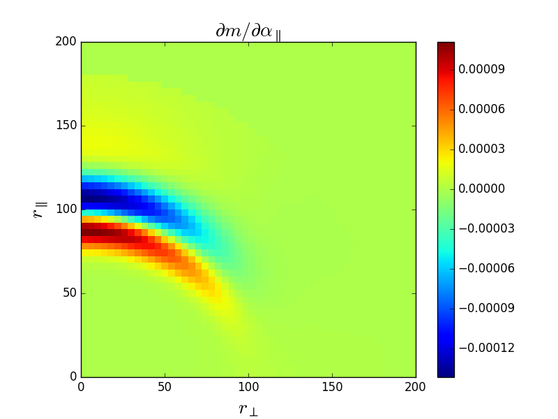
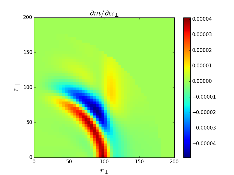
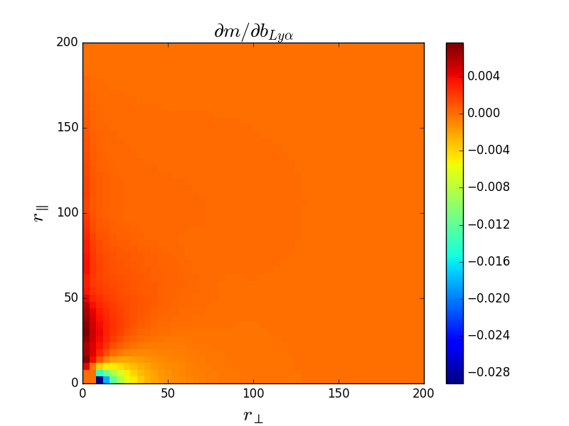
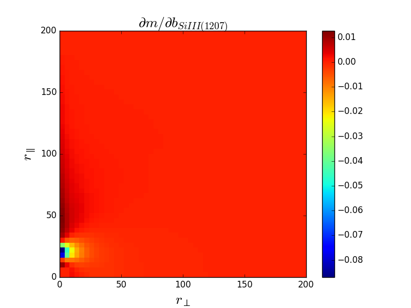
We represent the quantities for 4 of the 12 fitted parameters of the Lyauto-correlation function in Fig.13.
The covariance matrix then reads :
| (41) |
with
| (42) |
Since is symmetric, the determinant of the Fisher matrix, , does not depend on redshift and is given by:
| (43) |
The variance of at redshift becomes:
| (44) |
The effective redshift is the value which minimizes the error on :
| (45) |
i.e.,
| (46) |
In the case of a combined fit, we compute one matrix for each correlation function entering the fit:
| (47) |
where is the model for the correlation function at bin . In this case, reads:
| (48) |
Table 8 presents the effective redshifts at which the and parameters are measured for the different correlation functions computed in this paper. The effective redshift values differ by less than 0.5% for and . Figure 13 shows the quantities in the (, ) plane for the fitted parameters . is the baseline model for the Ly auto-correlation.
| Correlation functions | |||
|---|---|---|---|
| Ly(Ly) Ly(Ly) | 2.35 | 2.34 | 2.34 |
| Ly(Ly) Ly(Ly) | 2.29 | 2.29 | 2.28 |
| Ly(Ly)xLy(Ly+Ly) | 2.34 | 2.33 | 2.33 |
| Ly(Ly) Ly(Ly) (low z) | 2.19 | 2.19 | 2.18 |
| Ly(Ly) Ly(Ly) (high z) | 2.49 | 2.49 | 2.49 |
| Ly(Ly) Ly(Ly) | 2.76 | 2.77 | 2.78 |
Appendix B Fits in two redshift bins

The present data set is large enough to constrain the BAO parameters in two independent redshift bins, in a way similar to what will be done in forthcoming cosmological surveys, such as the DESI project (DESI Collaboration et al. 2016). To simplify the analysis, we consider only the Ly(Ly) Ly(Ly) correlation function.
A straightforward way of defining a high- and low-redshift sample of pixel pairs would be to simply use pixel pairs of mean redshift less than or greater than an appropriately chosen value, . The drawback of such an approach is that a given pair of forests could belong to both bins, as some pixels in a given forest would be associated with some pixels in the other forest, either in pixel pairs with mean redshift less than , or in pixel pairs with mean redshift greater than . The fact that some pairs of forests belong to both redshift bins introduces unwanted correlations when correcting for the distortions introduced by our continuum fitting procedure. To circumvent this problem, we choose to assign forest pairs to the high or low-redshift sample by cutting on the mean of the maximum of the two forests.
We thus evaluate, for all pairs of forests (), the following quantity:
| (49) |
where , with the last pixel of forest , and the rest-frame wavelength of the considered transition. The condition defines the low redshift bin, while the opposite condition defines the high redshift one.
The value of is tuned so that the sum of the weights of all absorber pairs in the high redshift correlation function equals the one of all pairs in the low redshift correlation function. This ensures the two bins have a comparable statistical power. This process leads us to select . The redshift distribution of absorber pairs obtained in this way are shown on Figure 14. The average pair redshift is and for the low and high redshift bin, respectively.


| Parameters | low z | high z |
|---|---|---|
| 1.008 0.043 | 1.088 0.046 | |
| 0.861 0.062 | 0.977 0.044 | |
| 2.083 0.160 | 1.585 0.113 | |
| -0.218 0.006 | -0.201 0.005 | |
| 0.745 0.174 | 0.678 0.179 | |
| -0.058 0.007 | -0.040 0.006 | |
| -0.0049 0.0015 | -0.0045 0.0016 | |
| -0.0067 0.0015 | -0.0021 0.0015 | |
| -0.0105 0.0016 | -0.0055 0.0017 | |
| -0.0039 0.0018 | -0.0021 0.0017 | |
| -0.0178 0.0095 | -0.0186 0.0095 | |
| 1580.95 | 1737.15 | |
| 1590 - 11 | 1590 - 11 | |
| Probability | 0.481 | 0.003 |
| 1584.30 | 1740.89 |
Figure 16 presents the result of fitting the Ly(Ly) Ly(Ly) correlation baseline model to the data in the low (blue points) and high (red points) redshift bins in the usual four wedges.
Table 9 shows the associated best-fit parameters. From the table, we note that is notably different at low and high redshift. When fitting the full sample, we assumed, following Kirkby et al. 2013, to be constant. A redshift dependent could thus be an improvement in future analyses.
From the lower right panel of Figure 16, we see that the amplitude of the high-redshift correlation function is higher than the amplitude of the low-redshift one. This is expected, as increases with redshift (Kirkby et al. 2013).
Figure 15 presents the constraints obtained, in the (,) parameter space, from fitting the Ly auto-correlation Ly(Ly)xLy(Ly) in the low (blue contours) and high (red contours) redshift bins. The values of corresponding to a given confidence level were taken from Table 12. Both the high and low redshift measurements are within of the Pl1015 model.
Appendix C The Ly(Ly)xLy(Ly) cross correlation
| Transitions | [] | |
|---|---|---|
| Si II(1190)/O VI(1038) | 1.147 | -88 |
| Si II(1193)/O VI(1038) | 1.150 | -81 |
| Si II(1190)/O VI(1032) | 1.154 | -73 |
| Si II(1193)/O VI(1032) | 1.156 | -66 |
| Si II(1190)/Ly(1026) | 1.161 | -56 |
| Si III(1207)/O VI(1038) | 1.163 | -52 |
| Si II(1193)/Ly(1026) | 1.163 | -50 |
| Si III(1207)/O VI(1032) | 1.169 | -37 |
| Ly(1216)/O VI(1038) | 1.172 | -31 |
| Si III(1207)/Ly(1026) | 1.176 | -20 |
| Ly(1216)/O VI(1032) | 1.178 | -16 |
| Si II(1260)/O VI(1038) | 1.215 | 68 |
| Si II(1260)/O VI(1032) | 1.221 | 83 |
| Si II(1260)/Ly(1026) | 1.229 | 100 |

| Parameters | Ly(Ly)xLy(Ly) |
|---|---|
| + Ly(Ly)xLy(Ly) | |
| + Ly(Ly)xLy(Ly) | |
| 1.840 0.084 | |
| -0.212 0.004 | |
| 1.123 0.384 | |
| -0.098 0.018 | |
| 1.116 0.152 | |
| -0.050 0.004 | |
| -0.073 0.005 | |
| -0.002 0.032 | |
| -0.0081 0.0015 | |
| -0.0055 0.0014 | |
| -0.0025 0.0005 | |
| -0.0022 0.0005 | |
| -0.0035 0.0005 | |
| -0.0011 0.0006 | |
| -0.0047 0.0025 | |
| 6469.77/(6360-15) | |
| Probability | 0.134 |

As an extension of our main analysis, we compute the Ly(Ly) Ly(Ly) correlation function, following the procedure previously described. We computed the 1D correlation function in the Lyregion (Fig 17) to identify the contaminating metals (see Table 10).
The results of this analysis are presented in Table 11. The Lyabsorption signal is clearly detected as is non zero at at the 2.9 level. We also see the signal due to O vi(1032) and O vi(1036). Note that the correlation between Lyand Si ii(1260) occurs near the BAO peak (last line of Table 10). Due to the small Lyabsorption cross-section and to the small wavelength extent of the Lyregion, it is harder to detect the BAO peak than for the Lyauto-correlation function. Moreover, the Ly-Si ii correlation further overlaps the BAO signal at small , hampering its detection in our data.
Figure 18 presents for the first time the 2D Ly(Ly) Ly(Ly) correlation function. It is shown in the usual four wedges of values, as a function of multiplied by the sign of . Note that the model is not symmetric around zero separation.
The oscillator strength of Lyabsorption is a fifth of that of Ly, and consequently there are far fewer LyHCD systems than LyHCD systems. On the other hand Lyabsorption in our analysis occurs at a systematically higher redshift. Overall we find that is consistent with zero.
In summary, there are not enough data at present to constrain the BAO peak position with Lyabsorption only. However, Lyabsorption could be used to access to physical IGM parameters at redshifts for which the Lyabsorption is saturated (Dijkstra et al. 2004, Iršič & Viel 2014).
Appendix D Confidence levels
To make a precise estimate of the relation between and confidence level, we followed closely the procedure of du Mas des Bourboux et al. 2017. We generated a large number of simulated correlation functions using the fiducial cosmological model and the best-fit values of non-BAO parameters, randomized using the covariance matrix measured with the data. Each simulated correlation function was then fit for the model parameters and the for the best-fit parameters compared with the best with one or more parameters set to the known input values. Confidence levels are the fractions of the generated data sets that have best fits below the limit. The uncertainties are estimated using a bootstrap technique.
The analysis of du Mas des Bourboux et al. 2017 followed this procedure using models that incorporated only Lyabsorption and models that incorporated also HCDs and metals. Since no significant differences were seen in the two methods, we use here only Lyabsorption, considerable simplifying the analysis.
The results are summarized in Table 12 for various correlation functions. In all cases the values corresponding to a given confidence level are increased above the standard values. For example, for the Ly(Ly) Ly(LyLy) correlation, the one- and two-standard deviation contours for correspond to and to be compared with the standard values of 2.29 and 6.18.
| Parameter | ||
|---|---|---|
| Ly(Ly) Ly(LyLy) | ||
| 1.19 0.03 | 4.74 0.09 | |
| 1.23 0.03 | 4.83 0.08 | |
| 2.77 0.04 | 7.33 0.10 | |
| Ly(Ly) Ly(LyLy) | ||
| + QSO Ly(LyLy) | ||
| 1.080.02 | 4.290.10 | |
| 1.080.02 | 4.280.10 | |
| 2.470.03 | 6.710.13 | |
| Ly(Ly) Ly(Ly) | ||
| 1.19 0.02 | 4.65 0.09 | |
| 1.17 0.02 | 4.32 0.07 | |
| 2.65 0.04 | 6.99 0.10 | |
| low z | ||
| 1.28 0.02 | 5.09 0.08 | |
| 1.35 0.02 | 5.09 0.10 | |
| 2.89 0.04 | 7.55 0.12 | |
| high z | ||
| 1.28 0.03 | 4.92 0.09 | |
| 1.23 0.03 | 4.74 0.08 | |
| 2.83 0.04 | 7.44 0.11 |