Spatially Extended Tests of a Neural Network Parametrization Trained by Coarse-grainingThanks: Department of Atmospheric Sciences, University of Washington, Box 351640, Seattle, WA 98195-1640
Abstract
General circulation models (GCMs) typically have a grid size of 25–200 km. Parametrizations are used to represent diabatic processes such as radiative transfer and cloud microphysics and account for sub-grid-scale motions and variability. Unlike traditional approaches, neural networks (NNs) can readily exploit recent observational datasets and global cloud-system resolving model (CRM) simulations to learn subgrid variability. This article describes an NN parametrization trained by coarse-graining a near-global CRM simulation with a 4 km horizontal grid spacing. The NN predicts the residual heating and moistening averaged over grid boxes as a function of the coarse-resolution fields within the same atmospheric column. This NN is coupled to the dynamical core of a GCM with the same resolution. A recent study described how to train such an NN to be numerically stable when coupled to specified time-evolving advective forcings in a single column model, but feedbacks between NN and GCM components cause spatially-extended simulations to crash within a few days. Analyzing the linearized response of such an NN reveals that it learns to exploit a strong synchrony between precipitation and the atmospheric state above . Removing these variables from the NN’s inputs stabilizes the coupled simulations, which predict the future state more accurately than a coarse-resolution simulation without any parametrizations of sub-grid-scale variability, although the mean state slowly drifts.
Journal of Advances in Modeling Earth Systems (JAMES)
Department of Atmospheric Sciences, University of Washington
nbren12@uw.edu
A neural network parametrization is coupled to a GCM
The neural network is trained by coarse-graining a near-global cloud-system resolving simulation
The coupled simulation accurately forecasts the weather of the training data
1 Introduction
Current global climate and weather models cannot explicitly resolve many important physical processes because of computational expenses. Global weather and short-range climate forecast models support grid sizes of (ECMWF 2018; NOAA 2018), while current climate models typically have grids. Unresolved processes, include cumulus convection, turbulence, and subgrid cloud variability are approximated by sub-grid-scale parametrizations (Palmer 2001). These are usually designed by human physical intuition, informed by process modeling and observations.
Cumulus convection in the tropics is one of the most dynamically important processes in the atmosphere yet it is extremely difficult to parameterize because of the multiscale nature of moist flows (Nakazawa 1988; Majda 2007). There is a long-standing debate about whether convective parametrizations should be based on moisture convergence or quasi-equilibrium closures Arakawa 2004. Moreover, important mean-state biases in climate modeling such as the double-ITCZ bias are sensitive to convective parametrization (Zhang and Wang 2006; Woelfle et al. 2018). Climate models also struggle to simulate observed aspects of tropical variability such as the diurnal cycle of continental precipitation (Stratton and Stirling 2012) and the Madden Julian Oscillation (MJO) (Jiang et al. 2015; Jiang 2017). Thus, an improved convective parametrization could help improve weather and climate simulations.
With sufficient computational resources, cloud-system resolving models (GCRMs) with sub- grid spacing can be run in global domains without deep convective parametrizations (Satoh et al. 2008; Bretherton and Khairoutdinov 2015). Recent studies have used such simulations to study the moist static energy budget (Bretherton and Khairoutdinov 2015) and cloud feedbacks (Narenpitak et al. 2017). The DYAMOND project recently compared 40-day hindcasts by 10 independently-developed global CRMs (CRMs), showing reassuring similarity in their simulated patterns of precipitation and high cloud (Stevens et al. Submitted). Centennial-scale climate GCRM simulations are not yet feasible, so improving parametrizations in coarse-resolution models remains an important goal.
It remains challenging for human experts to translate the vast volume of information in new high-resolution datasets and models into better parametrizations of moist physical processes incorporating subgrid variability. On the other hand, parametrizations can also be built using powerful regression tools developed in the field of machine learning (ML) (Rasp et al. 2018; O’Gorman and Dwyer 2018; Brenowitz and Bretherton 2018). In particular, Brenowitz and Bretherton 2018 trained a neural network (NN) (Goodfellow et al. 2016) parametrization for the combined diabatic heating and moistening in a coarse-grid model by coarse-graining a GCRM simulation. They showed that coupling this parametrization to specified dynamical tendencies in a single column model gives stable and highly accurate simulations if the NN is trained to optimize model performance over multiple time steps.
We now extend our single column model results by coupling an NN parametrization to the dynamical core of a GCM. As in Brenowitz and Bretherton 2018, this unified physics scheme will predict the sources of water and heat due to latent heating, turbulence, radiation, and any other physical process beyond resolved advection. Our main goal is to produce accurate multiple day forecasts with the coupled GCM-NN model.
After a brief survey of recent work on ML parametrization in Section 2, we describe our training data and GCM configuration in Section 3. Section 4 describes our coarse-graining and machine learning strategies. Particular focus is placed on the difficult task of ensuring numerical stability in spatially extended simulations (Section 4.3). Section 5 shows the results of the coupled simulations, and we conclude in Section 6.
2 Review of Machine Learning Parametrization
One attractive use of machine learning (ML) is to automatically tune existing GCM parametrizations, which build in physical insights and constraints that may help them apply across a range of climates. Proposed techniques include data assimilation (Schneider et al. 2017; Lyu et al.) and genetic algorithms (Langenbrunner and Neelin 2017). These techniques can tune a few free parameters, but may not scale to larger numbers of parameters. Moreover, existing parametrizations may not be flexible enough to be realistic in part because they have so few parameters. For instance, adjusting the entrainment rates in a convection scheme can improve mean-state bias, but harm the variability (Kim et al. 2011; Mapes and Neale 2011).
A more ambitious approach replaces an existing GCM parametrization with a machine learning (ML) model, which has enough parameters to capture arbitrarily complex relationships (Cybenko 1989; Hanin 2017) present within a training dataset. ML models are typically trained by minimizing a loss function, such as the mean-squared error (MSE) compared to some reference outputs from the training data; the choice of the loss function is subjective and a key to good performance. Early studies (Chevallier et al. 1998; Krasnopolsky et al. 2005) trained NNs (Goodfellow et al. 2016) to emulate the outputs of radiative transfer codes in order to decrease computational expense. Subsequent studies also trained NNs to emulate existing convective parametrizations (O’Gorman and Dwyer 2018) and super-parametrizations (SP) (Rasp et al. 2018). In each of these instances, the ML model is trained with a nearly ideal dataset, where the inputs are the state of the atmosphere, and the output is a tendency that has actually driven a GCM.
Training a parametrization by coarse-graining a GCRM is a more difficult problem because it lacks this hierarchical structure. On the other hand, GCRMs are the most realistic models available because they do not impose an arbitrary scale separation as SP does. In this setting, how does one define the target tendency? In the first study of its kind, Krasnopolsky et al. 2010; Krasnopolsky et al. 2013 defined the output as the residual heating and moistening (Yanai et al. 1973) in limited area simulations. They diagnosed heating rates and cloud fractions with high accuracy but did not present any prognostic simulations. Brenowitz and Bretherton 2018 extended this work in two ways. First, their training dataset was a near-global CRM with rich multiscale convective organization. Second, they found single column model (SCM) simulations with NNs trained in this way diverged to infinity after just a few time steps. They ensured long-term stability by minimizing the loss accumulated over several predicted time steps.
In summary, in coarse-graining, there is no clear target to emulate. While Brenowitz and Bretherton 2018 developed an approach for ensuring numerical stability in a single-column mode with prescribed dynamics, they did not test it within a full three-dimensional GCM where the dynamics interact with the NN parametrization.
3 Training Data and Atmospheric Model Configuration
3.1 Training Data
We use the same training dataset as Brenowitz and Bretherton 2018: a near-global aquaplanet simulation (NG-Aqua) using the System for Atmospheric Modeling (SAM) version 6.10 (Khairoutdinov and Randall 2003). SAM is run in a cloud-system resolving configuration with a horizontal grid spacing of in a tropical channel domain measuring zonally by meridionally. The simulation has 34 vertical levels with a spacing that increases from at the surface to in the troposphere and stratosphere. The atmospheric circulation is driven by a zonally symmetric sea surface temperature (SST) profile which peaks at at the equator () and decreases to at the poleward boundaries. Because SAM was originally designed for small-scale modeling, the grid is Cartesian and no spherical effects are included, except for a meridionally varying Coriolis parameter. Despite the simplifications described above, NG-Aqua features realistic multiscale organization of tropical and midlatitude systems.
The simulation uses the radiation scheme from version 3 of the Community Atmosphere Model (CAM) with a zonally symmetric diurnal cycle and a bulk microphysics scheme (Khairoutdinov and Randall 2003). It was initialized with small random perturbations to the temperature, spun up on a 20 km grid, then interpolated to 4 km and run for 100 days, storing the full 3-D outputs every 3 hours. To allow for the circulation to statistically equilibrate at , all analyses described below are performed on the final 80 days. More details about the model configuration are described by Brenowitz and Bretherton 2018 and Narenpitak et al. 2017.
3.2 Coarse-resolution model configuration
We test the NN schemes within an atmospheric model with a grid resolution of , which is within the range of modern GCMs. This scale is coarse enough that the grid-mean precipitation has significant auto-correlation over the 3-hour sampling interval of the training data, which should therefore sufficiently resolve the time-evolving grid-mean moist convective dynamics.
We use SAM rather than a more traditional GCM as our coarse-grid model to ensure that it has the same geometry and dry dynamics as the training data. This model, coarse-SAM (cSAM), is run with the same vertical grid as the NG-Aqua simulation. Its default microphysics scheme has the same three prognostic thermodynamic variables as SAM: the total non-precipitating water mixing ratio , the precipitating water mixing ratio , which is a fast variable that we will neglect in the parametrizations below; and the liquid-ice static energy . See (Khairoutdinov and Randall 2003, Appendix A) for more details.
SAM is typically used for cloud-resolving simulations so running it efficiently and stably with coarse resolution required several modifications. Most importantly, horizontal hyper-diffusion of , , and the three wind components, , , and , was added to suppress grid-scale oscillations and model blow-up (divergence of the solutions to machine infinity in a finite amount of time). For the 160 km grid, was sufficient to damp grid-scale oscillations.
For NN simulations, we use a simplified momentum damping rather than SAM’s default turbulence closure, which severely limits the time step on the 160 km grid. This forcing damps the velocity towards zero at a rate which decreases linearly from at the surface to zero at a -level of (Held and Suarez 1994). Because this is different than NG-Aqua, it leads to an inevitable drift of cSAM simulations away from NGAqua over the course of a few days. In the future, we hope to use learned coarse-grained momentum tendencies from NG-Aqua in place of this approach.
We compare simulations with cSAM coupled to our NN parametrization with a base version of cSAM with the microphysics and radiation tendencies calculated from grid-scale mean thermodynamics. Unlike the NN simulations, the surface fluxes are computed interactively and coupled to SAM’s default turbulence scheme. The base cSAM will only precipitate when a coarse-resolution grid-cell achieves saturation, so we expect it will produce noisy simulations. Ideally, we would have preferred to compare the NN parametrizations against a traditional GCM parametrization suite, as did Rasp et al. 2018 and Brenowitz and Bretherton 2018, but no such scheme has been implemented in SAM.
In this article, we assess the accuracy of 10-day weather simulations. They are initialized with the coarse-grained outputs from a particular time, day 100.625, of the NG-Aqua simulation. Our goal is to obtain cSAM simulations that best match the actual evolution of NG-Aqua over the following 10 days. All of the simulations presented in this paper use a timestep. The thermodynamic variables and vertical velocity from the 4 km NG-Aqua data, are averaged over grid cell blocks, but the horizontal velocities must be averaged along the interfaces of these blocks to respect the anelastic mass conservation equation.
4 Machine Learning Parametrization
4.1 Coarse-graining Problem
An NN will parameterize the unknown sources of the thermodynamic variables and . Their coarse-resolution budgets are given by
| (1) | ||||
| (2) |
where is the horizontal average of over the coarse-grid boxes. The first term on the right-hand side of these budgets are the tendencies due to the GCM, which includes advection and any other explicitly treated process. The apparent heating and moistening are defined as a budget residual from these GCM tendencies (Yanai et al. 1973). Because they are residuals, they contain the effects of all unresolved and untreated physics including latent heating, turbulent mixing, and radiation.
The goal of any parametrization is to approximate and as potentially stochastic and non-local functions of the coarse resolution variables alone (Palmer 2001). Because radiative heating and moist physical processes couple the atmosphere more strongly in the vertical than the horizontal direction, we follow the assumption of horizontal locality typically made in moist physics parametrizations; this reduces the dimensionality of the training problem, allowing robust results to be obtained from our NG-Aqua training dataset. For simplicity, we also treat and as deterministic functions of the inputs.
The inputs are the vertical profiles of the prognostic variables and , as well as the sea surface temperature (SST) and downwelling insolation (SOLIN) at the top of the atmosphere, which are external parameters. Unlike Brenowitz and Bretherton 2018, we do not use latent heat flux because it depends on the surface winds, which tend to be inaccurate because they are forced by the simplified damping scheme described in Section 3 rather than a coarse-grained source from NG-Aqua.
Let the vector concatenate the observed prognostic variables and over all coarse-grained grid levels in grid column , and let contain the auxiliary variables SST and SOLIN at this location. With these assumptions, (1) and (2) can be combined:
| (3) |
where the subscript is the index of the given horizontal grid cell and the superscript indicates that these are observed quantities. The function and its parameters are invariant for all locations. Here, is the GCM tendency from coarse-grid advection (which involves other grid columns and hence is nonlocal); is the portion of the apparent sources and that can be modeled deterministically, which the NN will be used to parameterize; and includes stochastic and structural error. As with Brenowitz and Bretherton 2018, will be parameterized as an NN where the parameters include the weights and biases of the network’s layers.
4.2 Loss Functions for Numerically Stable Parametrizations
How do we find the parameters from the NG-Aqua time series ? Brenowitz and Bretherton 2018 trained a numerically stable NN for use in single column model (SCM) simulations by minimizing the multiple step prediction error (MSPE) over a 1-3 day prediction window . SCM dynamics decouple the dynamics of an atmospheric column from its surroundings and are described mathematically by
| (4) |
where is the single column time series for a given location , starting prediction time , and set of parameters . Compared to (3), the global state and the auxiliary variables are prescribed functions of time, which are decoupled from the local dynamics.
Brenowitz and Bretherton 2018 define the MSPE as
| (5) |
where the sum ranges over all possible prediction start times and spatial locations . The inner norm is given by
| (6) |
where is SAM’s reference density profile. is the mass of an atmospheric column while and are weight constants for the temperature and humidity, respectively. In this study, we find that when setting and each variable contributes comparably to the overall loss. This resulted in a highly accurate single column time-stepping scheme which closely replicated the and time series of the NG-Aqua data.
Unfortunately, MSPE training produces NN schemes which implicitly depend on the temporal discretization and time step used to simulate (4). The main symptom of this is a “spin-up” error where the SCM only produces accurate tendencies after a few time steps of prediction (see Figure 1): the spun-up predictions (panel c, d) more closely resemble the truth (panel a) than the instantaneous prediction (b) does. Because this spin-up process occurs after 3 hours, it did not cause large errors in the single column simulations of Brenowitz and Bretherton 2018. However, for spatially-extended simulations, the coupling between the GCM dynamics and the NN occurs at every time step, so the NN must produce accurate predictions from the start. Thus, MSPE-trained NNs are not suitable for use within cSAM because they spin-up on a time-scale longer than the cSAM time step.
Our goal in this article is to develop a loss function which produces an NN that gives spatially-extended coarse-grid simulations that are stable, unbiased, and insensitive to the model time step. This loss function is inspired by the Lax equivalence theorem in numerical analysis, which asserts that a finite difference method is accurate if and only if it is consistent and stable (Quarteroni et al. 2007). The loss is given by
| (7) |
Consistency will mean that the approximates and instantaneously, and is accomplished by minimizing the loss given by
| (8) | ||||
| (9) |
In practice, the storage terms are estimated from the 3 hourly sampled data using finite differences. Thus, minimizing demands that approximates the apparent heating and moistening.
On the other hand, stability requires that the small perturbations to the inputs do not grow under the dynamics given by (4). In practice, we enforce this using a penalty given by
| (10) |
where is the time average operator. is the single column simulation under the action of the time-mean forcing, whose dynamics are given by
| (11) |
Its initial condition is . This penalty demands that the SCM simulation does not diverge too quickly for a prediction of length (). Because uses constant forcing, it is less sensitive than the MSPE to the temporal discretization of (4). In practice, NNs trained to minimize avoid spin-up errors and accurately predict and at the initial time. Like MSPE-trained NNs, they do produce stable, albeit less accurate, SCM simulations. Since our main goal is to produce accurate coupled GCM-NN simulations this deteriorated SCM performance is acceptable.
4.3 Coupled Numerical Instability


The methods discussed still do not prevent model blow-up when coupled to cSAM, as we will show in Section 5. This occurs because the single column training strategy does not account for feedbacks between cSAM and the NN so corresponding numerical instabilities are not penalized.
A similar feedback causes grid-scale storms when a GCM is coupled to a moisture-convergence closures (Arakawa 2004). Emanuel et al. 1994 argue this closure fundamentally confuses cause and effect, and that precipitation drives moisture convergence rather than vice versa. In fact, such misleading correlations are common in nonlinear dynamical systems such as the atmosphere, a phenomenon known as synchronization (Pecora et al. 1997), so data-driven models must be taught to ignore such non-causal correlations. Thus, we must determine if the NN is mistaking cause for effect.
4.3.1 Interpreting the trained networks using linear response functions
The linearized response of the NN to small perturbations can reveal if it is confusing cause and effect. The linearized response function (LRF) is given by
where the derivative is with respect to the phase space variables . For ease of discussion, we defer the model architecture and training details to Section 4.4. We first train an NN using the stability-penalized loss in (7) and then compute its LRF for the mean equatorial sounding (Figure 2) using automatic differentiation (Paszke et al. 2017). We compare against LRFs that Kuang 2018 computed by perturbing the steady forcing of a CRM, which presumably represent causal relationships between the inputs and outputs.
Are the LRFs of our NNs similar to those of Kuang 2018? The LRFs of Kuang 2018 have an upward dependence structure (a mainly upper-triangular structure in the panels of Figure 2), where the heating and to a lesser extent, the moistening, at a given vertical level depend only on data from below. This is physically realistic since cumulus convection initiates at lower elevations and deepens into cumulonimbus; evaporation of precipitation leads to some low-triangular structure as well. On the other hand, our NN predicts that heating and moistening at all heights are very sensitive to the humidity near the tropopause (200 mb), a physically nonsensical result. A increase of humidity at this level leads to more than of drying at all lower levels. Moreover, the NN does not accurately predict and at these levels (cf. Figure 5), perhaps because the fluctuations of humidity and temperature at these levels occur on faster time-scales than the 3-hour sampling rate of the data. Thus, the NN depends most sensitively on the inputs that it performs worst on.
The NN is sensitive to upper-level humidity because the latter is strongly correlated to precipitation. Figure 3a shows that the humidity and apparent moistening are highly anticorrelated, as measured by the effective damping rate given by
| (12) |
where is the zonal and time averaging operator. Near the tropopause, the moisture has a damping time-scale of , which is the sampling rate of the NG-Aqua data. This strong damping results in a near perfect correlation between the advective moistening and at this level, as shown in Figure 3b.
The advective moistening is primarily driven by grid-scale mean vertical motions due to cumulus convection. The numerical instability probably appears in the tropics first because the weak temperature gradient there ensures that latent heating drives grid-scale average vertical motions (Sobel and Bretherton 2000). Thus, the amount of water cSAM advects into the upper atmosphere strongly correlates with precipitation.
The sensitivity to humidity can drive numerical instability as follows. A positive moisture anomaly in the tropical upper troposphere will increase the predicted precipitation and heating. This will then increase the upward velocity, which closes the feedback loop by increasing the supply of moisture to the upper atmosphere. Ultimately, this feedback can lead to grid-scale storms (see Figure 7c below), similarly to moisture convergence closures.
This instability might be less problematic had we been able to customize the 4 km NG-Aqua simulations for the training process so as to better infer causality, e. g. by using higher output time resolution and calculation of instantaneous heating and moistening rates. However, we were forced to work around it, as described in the next section.
4.3.2 Eliminating non-causal relationships
We enforce a more plausible causal structure on the NN by not using the humidity and temperature above certain heights as predictors. To obtain a numerically stable simulation without grid-scale storms, it suffices to ignore the and at or above levels 15 () and 19 (), respectively. We also assume that that the NN predicts at the same levels; however, a debiasing procedure discussed below will allow predictions of non-zero tendencies there. To justify this assumption, we note that is small at these levels, and that is very noisy above (cf. Figure 6). We have run cSAM simulations with this configuration for up to 100 days without numerical blow-up or grid-point storms.
Figure 4 shows the LRF of the modified NN. Most strikingly, the linearized response of the drying/moistening to the input variables is an order of magnitude smaller than for the NN with all input variables. For the most part, this LRF also has a smoother vertical structure that is more compatible with the CRM derived LRFs (Kuang 2018). For instance, both our LRFs and those of Kuang 2018 show that destabilizing the atmosphere by decreasing the lower tropospheric temperature leads to heating/drying throughout the column (panels b and d). Likewise, the lower tropospheric moisture induces convective heating above (panel c). Unfortunately, there are still large oscillations in the response of to the humidity at . Nonetheless, ignoring the upper atmospheric variables markedly improves the linearized response of the NN.
4.4 Network architecture and training
Unlike Rasp et al. 2018, we did not find that changing network architecture by adding more layers or parameters prevents blow-up. However, since we are training the data with global data, we use a higher capacity network than Brenowitz and Bretherton 2018 used for the tropics alone. Thus, each model trained in this paper has three densely connected hidden layers with 256 nodes each and rectified linear unit (ReLU) activations. Altogether, this architecture has free parameters.
Prior to input, each input variable is normalized by the global mean and dividing by the standard deviation for each level independently, except where the latter vanishes. This level-by-level normalization is a departure from past studies (Rasp et al. 2018; Brenowitz and Bretherton 2018), but had little impact upon the results. In particular, NNs trained with inputs normalized as Brenowitz and Bretherton 2018 also learn to depend strongly on the upper atmospheric humidity and suffer from coupled numerical instabilities discussed above.
The networks weights and biases are optimized by stochastic gradient descent (SGD) with the popular Adam (Kingma and Ba 2014) optimizer with an initial learning rate of . If a sample is defined as an individual atmospheric column for a given horizontal location and time step, then there are samples in the training dataset. These samples are randomly in horizontal space and formed into batches of 64 time series, each containing the full 80 days of data. In practice, SGD trains an NN that captures the time-space variability in diabatic processes, but makes large () errors in the zonal and time mean. This occurs because of the optimization is highly non-convex and the variability of cloud-related processes is larger than its mean. Therefore, after SGD converges, we use linear regression to de-bias the predicted heating and moistening for each height and latitude separately (see Text S1). To avoid re-introducing the causality and numerical stability issues solved in Section 4.3, these regressions depend only the predictions of and as well as and at the given height and do not introduce new dependencies between vertical levels.
The NN training and linear regression are implemented in Python using PyTorch (Paszke et al. 2017) and scikit-learn (Pedregosa et al. 2011), respectively. The debiased NN models are then coupled to cSAM using a python interface. The predicted tendencies are disabled within 3 grid cells () of the boundary because the flow in these regions is greatly influenced by the no-normal flow boundary conditions, so the NN is inaccurate there (cf. Fig. 5).
5 Results

We now present our spatially-extended simulations. As described in Section 3, the simulations are initialized with the NG-Aqua data at day 100.625, and our discussion focuses on the prediction accuracy in the first 10 forecast days. Two NN parametrizations will be compared with the training data and the base simulation with resolved-scale microphysics and radiation. The first NN simulation, labeled as “NN-All”, is performed using the NN which includes all levels as input. The discussion in Section 4.3 indicates that this setup leads to grid-scale storms and model blow-up. The NN in the second simulation, known as “NN-Lower”, only uses humidities below level 16 (375 mb) and temperature below level 19 (226 mb) as described in Section 4.3.2. When evaluated directly on the NG-Aqua data, NN-Lower has an value of around 60% for and in the lower troposphere (Figure 5). Interestingly, the predicted heating and moistening are less noisy than the “true” values estimated as budget residuals (Figure 6). Thus, the NN-Lower parametrization performs well in an instantaneous sense.
Figure 7b demonstrates that the NN-Lower configuration is indeed numerically stable and produces a reasonable prediction of the PW after 5 days, albeit with a visible loss in large-scale moisture variability in the tropics. On the other hand, NN-All shows extremely moist grid-scale storms near the tropics, which coincide with intense precipitation and ascent (not shown). Likewise, the base simulation suffers from grid-point storms in the tropics and frontal regions in the extratropics, and it ultimately blows up after 9 days of simulation.
5.1 Perfect Model Weather Prediction

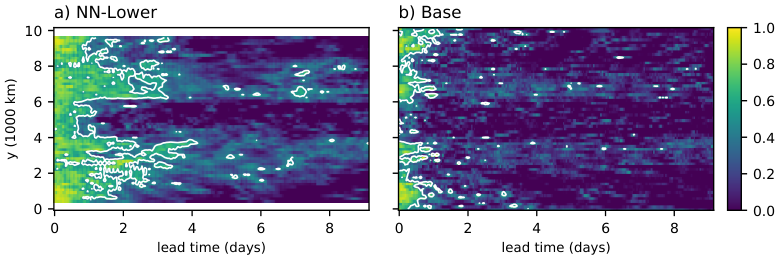
Figure 8 shows the root-mean-squared error (RMSE) of , , and the vertical component of vorticity for each configuration. The RMSE values are vertically integrated and mass-weighted and averaged over different latitude bands. The tropics lie within of the equator, the sub-tropics are between and , and the extra-tropics are the poleward of the domain. For all regions and variables, NN-Lower has the lowest RMSE. This improvement is most striking for the thermodynamic variables and , which have parameterized source terms. Compared to the base simulation, NN-Lower has 50% lower errors in both and . The vorticity error improves less, which is not surprising since we do not attempt to correctly represent the source of momentum (). However, in the extra-tropics, both NN-Lower and NN-All outperform the base simulation. Overall, NN-Lower produces the most accurate predictions.
The NN-Lower simulation also predicts the net precipitation rate more accurately than the base simulation does. The net precipitation rate is given by
where is precipitation and is the evaporation (Yanai et al. 1973). Net precipitation is the closest analog to precipitation that the NNs can predict because they predict the combined effect of precipitation and evaporation.
The net precipitation is much less noisy than in NN-Lower than the base run. Figure 9 shows maps of net precipitation after two days of prediction (day 102.625) for the NG-Aqua training data and the NN-Lower and base simulations. Overall, the NN-Lower simulation produces the correct extra-tropical pattern of net precipitation, but fails to produce enough variability in the tropics. In NG-Aqua, the tropical precipitation occurs in small-scale clusters and in a larger-scale Kelvin wave centered around at day 102.625, elsewhere there is column moistening due to evaporation. On the other hand, the base simulation produces far too strong and noisy precipitation, as expected for a scheme which only rains when a large-scale grid-cell becomes saturated.
Does the NN predict overly smooth net precipitation at the initial time or does this smoothness only appear as the coupled simulation evolves? The NN’s “semi-prognostic” net precipitation (i.e. predicted from the true coarse-grained NG-Aqua state at that time) is also shown in Figure 9b. Even in this instantaneous sense, the NN-Lower prefers to lightly rain throughout the tropics, rather than moisten in certain regions and strongly dry in others.
Figure 10 shows the pattern correlation compared to NG-Aqua of net precipitation for the NN-Lower and base simulations. NN-Lower has higher pattern correlations than the base simulation at all times and retains a correlation of 0.5 up to day 101.5 in the tropics and beyond day 102.5 in the extra-tropics and sub-tropics. By this measure, the base simulation has little predictive skill in the tropics.
5.2 Mean-state bias

Short-term predictions with NN-Lower are reasonably accurate, but the mean state drifts away from the true climate. We first focus on the time evolution of the zonal mean precipitable water (PW) and net precipitation, as shown in Figure 11. The fields are shown for days 100-120 for NG-Aqua and the NN-Lower simulation; the base simulation crashed in day 110. Compared to NG-Aqua, NN-Lower maintains the correct meridional distribution of PW, but the net precipitation steadily decreases in the tropics. All else equal, this would tend to increase the PW in the tropics, but the Hadley circulation and its transport of vapor towards the equator also weaken. On the other hand, the net precipitation in the base simulation becomes too concentrated at the equator and atmosphere dries out significantly. Overall, NN-Lower outperforms the base case and maintains the correct zonal-mean PW distribution, but does not produce enough precipitation in the tropics at later times.
Figure 12 shows the zonal-mean bias vs. NG-Aqua for the zonal winds, meridional streamfunction, humidity , and temperature in the NN-Lower simulation, time-averaged over forecast days 5–10. The humidity bias is relatively small with an amplitude of less than . The bias of is also small, and peaks near the meridional boundaries of the domain where the NN is not used. On the other hand, the meridional circulation substantially weakens from a peak mass transport of to . This is associated with the decreasing in the tropics seen in Figure 11. The zonal mean zonal winds also differ substantially. The surface westerlies and eddy-driven-jets become weaker, likely due to the Held-Suarez momentum damping. At the same time, the jets shift southward and super-rotation develops near , likely as a transient response to the weakening Hadley circulation. Overall, the small biases in the thermodynamic variables and belie growing biases in the circulation.
The loss of zonal variability in net precipitation (Fig. 9) and precipitable water (Fig. 7) might explain these mean-state drifts. Precipitation depends exponentially on precipitable water (Rushley et al. 2018; Bretherton et al. 2004), therefore a reduction in the zonal variance of PW (fewer extremely moist or dry coarse grid cells) will tend to decreases the zonal-mean precipitation for a given zonal-mean PW. Figure 13 confirms that this occurs in the NN-Lower simulation, whose mean tropical net precipitation is 40% weaker than NG-Aqua despite having a similar mean PW. Indeed, Figure 13 shows that the joint distribution of PW and net precipitation has much less variance in NN-Lower than in NG-Aqua.
The predicted net precipitation has too little variance even when evaluated on the true state (Fig. 13c). In other words, the distribution of net precipitation has too little spread for a given value of PW— i.e. the NN relies too strongly on PW. When integrated forward in time, this lack of variance likely reduces the PW variance, and therefore the mean precipitation. Thus, enhancing the variance of the conditional distributions of net precipitation could ameliorate the circulation biases in these simulations.
Plausible physical mechanisms for the loss of moisture variability depend on the spatial scale. On smaller scales, both the explicit hyper-diffusion and implicit numerical diffusion could reduce the variance of moisture. For larger scales, the moisture probably varies less because NN-Lower prefers to smooth throughout the tropics rather than delineating precipitating and evaporating regions. Future work could improve this by developing a stochastic or deterministic trigger for convection, or by separating precipitating and evaporating processes.
6 Conclusions
We use a neural network to build a unified physics parametrization of diabatic heating and moistening, which include the effects of unresolved subgrid processes. The neural network is trained by coarse-graining a near global aquaplanet simulation with a grid size of to a resolution of . It learns the coarse-grid heating and moistening profiles, calculated as residuals from the coarse-grid dynamics, from the temperature and moisture profiles, plus auxiliary parameters. A key challenge of the coarse-graining approach is that it lacks the natural hierarchical structure of other training datasets used in the literature, such as super-parametrization (SP) (Rasp et al. 2018). In the SP application, for instance, the target model and the training model share the same software interface for the physical process tendencies. These tendencies are predicted by a high-resolution submodel in the SP training dataset and must be learned by the neural network parametrization for application to the target model. This application is thus a clear target for emulation.
We extend the single column model results of Brenowitz and Bretherton 2018 to a spatially-extended simulation. The coarse-grid dynamical core is the same anelastic atmospheric model that generated the 4 km training dataset but is run with a resolution. This model needed additional damping in the form of horizontal hyper-diffusion and Newtonian relaxation near the surface to run stably in a base configuration with its default resolved-scale microphysics and radiation schemes, or with our neural network unified-physics parametrization. We developed a deeper version of our neural network capable of simulating the diabatic heating and moistening over the entire 46S-46N domain of our training simulations, rather than just the tropical subdomain used by Brenowitz and Bretherton 2018. We include a zonal-mean bias correction to minimize zonal mean temperature and moisture drifts.
An attempt to couple a preliminary version of this neural network to this GCM caused the model to blow up. Analyzing the linearized response of that neural network showed that it inadvertently learns to exploit a strong correlation between upper atmospheric humidity and precipitation. This correlation owes to the short lifetime of water vapor at those heights rather than any causal mechanism. Thus, ML parametrization is not immune to issues with causality that have long inspired debates about closure assumptions.
We enforced a plausible causal structure by removing the upper atmospheric humidity and temperature from the neural network inputs. Spatially extended simulations with this modified network can run stably indefinitely, without blowing up. Thus, stabilizing the parametrization required a rather crude human intervention. Future studies will need to explore automatic ways to discover true causal relationships and forestall model blow-up in a dynamically coupled setting.
The resulting neural network predicted the weather of NG-Aqua with much higher forecast skill and lower bias than a base coarse-grid simulation with only resolved microphysics and radiation parametrizations, which is the only reference case we could easily use as a metric. For a fair comparison, we will need to train and implement the ML parametrization in a global model whose coarse-grid version is typically run with a traditional suite of physical parametrizations.
More work is needed to reduce the long-term biases in these simulations. While temperature and humidity biases are small in the first 10 days, the Hadley circulation is dramatically weakened because there is not enough heating in the tropics to sustain vertical motions. Thus, more work is needed to keep the climate generated by neural network parametrizations trained by coarse-graining from drifting. We argue that our scheme could benefit from adding a mechanism for enhancing the tropical variance of moisture and the predicted precipitation, such as stochasticity in the parametrized tendencies.
Acknowledgements.
N.B. is supported as a postdoctoral fellow by the Washington Research Foundation, and by a Data Science Environments project award from the Gordon and Betty Moore Foundation (Award #2013-10-29) and the Alfred P. Sloan Foundation (Award #3835) to the University of Washington eScience Institute. C.B. is supported by U. S. Department of Energy grants DE-SC0012451 and DE-SC0016433. The coarse-grained NG-Aqua data and computer codes are available atzenodo.org (Brenowitz 2018; Brenowitz 2019a) and GitHub (Brenowitz 2019b), respectively.
References
- Arakawa (2004) Arakawa, A. (2004), The cumulus parameterization problem: Past, present, and future, J. Clim., 17(13), 2493–2525, 10.1175/1520-0442(2004)017¡2493:RATCPP¿2.0.CO;2.
- Brenowitz (2018) Brenowitz, N. D. (2018), Coarse-grained outputs from near-global aqua-planet control run with QOBS SST, 10.5281/zenodo.1226370.
- Brenowitz (2019a) Brenowitz, N. D. (2019a), Coarse-grained near-global aqua-planet simulation with computed dynamical tendencies, 10.5281/zenodo.2621638.
- Brenowitz (2019b)
Brenowitz, N. D. (2019b),
https://github.com/nbren12/uwnetv0.7, 10.5281/zenodo.2621717. - Brenowitz and Bretherton (2018) Brenowitz, N. D., and C. S. Bretherton (2018), Prognostic validation of a neural network unified physics parameterization, Geophys. Res. Lett., 17, 2493, 10.1029/2018GL078510.
- Bretherton and Khairoutdinov (2015) Bretherton, C. S., and M. F. Khairoutdinov (2015), Convective self-aggregation feedbacks in near-global cloud-resolving simulations of an aquaplanet, Journal of Advances in Modeling Earth Systems, 7(4), 1765–1787.
- Bretherton et al. (2004) Bretherton, C. S., M. E. Peters, and L. E. Back (2004), Relationships between water vapor path and precipitation over the tropical oceans, J. Clim., 17(7), 1517–1528, 10.1175/1520-0442(2004)017¡1517:RBWVPA¿2.0.CO;2.
- Chevallier et al. (1998) Chevallier, F., F. Chéruy, N. A. Scott, and A. Chédin (1998), A neural network approach for a fast and accurate computation of a longwave radiative budget, J. Appl. Meteorol., 37(11), 1385–1397, 10.1175/1520-0450(1998)037¡1385:ANNAFA¿2.0.CO;2.
- Cybenko (1989) Cybenko, G. (1989), Approximation by superpositions of a sigmoidal function, Math. Control Signals Systems, 2(4), 303–314, 10.1007/BF02551274.
- ECMWF (2018) ECMWF (Ed.) (2018), Part III : Dynamics and numerical procedures, no. 3 in IFS Documentation, ECMWF.
- Emanuel et al. (1994) Emanuel, K. A., J. David Neelin, and C. S. Bretherton (1994), On large-scale circulations in convecting atmospheres, Q.J.R. Meteorol. Soc., 120(519), 1111–1143, 10.1002/qj.49712051902.
- Goodfellow et al. (2016) Goodfellow, I., Y. Bengio, and A. Courville (2016), Deep learning, Adaptive computation and machine learning, The MIT Press, Cambridge, Massachusetts.
- Hanin (2017) Hanin, B. (2017), Universal function approximation by deep neural nets with bounded width and ReLU activations, arXiv e-prints.
- Held and Suarez (1994) Held, I. M., and M. J. Suarez (1994), A proposal for the intercomparison of the dynamical cores of atmospheric general circulation models, Bull. Am. Meteorol. Soc., 75(10), 1825–1830, 10.1175/1520-0477(1994)075¡1825:APFTIO¿2.0.CO;2.
- Jiang (2017) Jiang, X. (2017), Key processes for the eastward propagation of the Madden-Julian oscillation based on multimodel simulations, J. Geophys. Res. D: Atmos., 122(2), 2016JD025,955, 10.1002/2016JD025955.
- Jiang et al. (2015) Jiang, X., D. E. Waliser, P. K. Xavier, J. Petch, N. P. Klingaman, S. J. Woolnough, B. Guan, G. Bellon, T. Crueger, C. DeMott, C. Hannay, H. Lin, W. Hu, D. Kim, C.-L. Lappen, M.-M. Lu, H.-Y. Ma, T. Miyakawa, J. A. Ridout, S. D. Schubert, J. Scinocca, K.-H. Seo, E. Shindo, X. Song, C. Stan, W.-L. Tseng, W. Wang, T. Wu, X. Wu, K. Wyser, G. J. Zhang, and H. Zhu (2015), Vertical structure and physical processes of the Madden-Julian oscillation: Exploring key model physics in climate simulations, J. Geophys. Res. D: Atmos., 120(10), 2014JD022,375, 10.1002/2014JD022375.
- Khairoutdinov and Randall (2003) Khairoutdinov, M. F., and D. A. Randall (2003), Cloud resolving modeling of the ARM summer 1997 IOP: Model formulation, results, uncertainties, and sensitivities, J. Atmos. Sci., 60(4), 607–625, 10.1175/1520-0469(2003)060¡0607:CRMOTA¿2.0.CO;2.
- Kim et al. (2011) Kim, D., Y.-S. Jang, D.-H. Kim, Y.-H. Kim, M. Watanabe, F.-F. Jin, and J.-S. Kug (2011), El niño-southern oscillation sensitivity to cumulus entrainment in a coupled general circulation model: ENSO SENSITIVE TO CONVECTION SCHEME, J. Geophys. Res., 116(D22), 10.1029/2011JD016526.
- Kingma and Ba (2014) Kingma, D. P., and J. Ba (2014), Adam: A method for stochastic optimization.
- Krasnopolsky et al. (2005) Krasnopolsky, V. M., M. S. Fox-Rabinovitz, and D. V. Chalikov (2005), New approach to calculation of atmospheric model physics: Accurate and fast neural network emulation of longwave radiation in a climate model, Mon. Weather Rev., 133(5), 1370–1383, 10.1175/MWR2923.1.
- Krasnopolsky et al. (2010) Krasnopolsky, V. M., M. S. Fox-Rabinovitz, and A. A. Belochitski (2010), Development of neural network convection parameterizations for numerical climate and weather prediction models using cloud resolving model simulations, in The 2010 International Joint Conference on Neural Networks (IJCNN), pp. 1–8, 10.1109/IJCNN.2010.5596766.
- Krasnopolsky et al. (2013) Krasnopolsky, V. M., M. S. Fox-Rabinovitz, and A. A. Belochitski (2013), Using ensemble of neural networks to learn stochastic convection parameterizations for climate and numerical weather prediction models from data simulated by a cloud resolving model, Advances in Artificial Neural Systems, 2013, e485,913, 10.1155/2013/485913.
- Kuang (2018) Kuang, Z. (2018), Linear stability of moist convecting atmospheres part i: from linear response functions to a simple model and applications to convectively coupled waves, J. Atmos. Sci., 10.1175/JAS-D-18-0092.1.
- Langenbrunner and Neelin (2017) Langenbrunner, B., and J. D. Neelin (2017), Pareto-Optimal estimates of california precipitation change, Geophys. Res. Lett., p. 2017GL075226, 10.1002/2017GL075226.
- (25) Lyu, G., A. Köhl, I. Matei, and D. Stammer (), Adjoint-Based climate model tuning: Application to the planet simulator, J. Adv. Model. Earth Syst., 10.1002/2017MS001194.
- Majda (2007) Majda, A. J. (2007), Multiscale models with moisture and systematic strategies for superparameterization, J. Atmos. Sci., 64(7), 2726–2734, 10.1175/JAS3976.1.
- Mapes and Neale (2011) Mapes, B., and R. Neale (2011), Parameterizing convective organization to escape the entrainment dilemma, J. Adv. Model. Earth Syst., 3(2), M06,004, 10.1029/2011MS000042.
- Nakazawa (1988) Nakazawa, T. (1988), Tropical super clusters within intraseasonal variations over the western pacific, Journal of the Meteorological Society of Japan. Ser. II, 66(6), 823–839.
- Narenpitak et al. (2017) Narenpitak, P., C. S. Bretherton, and M. F. Khairoutdinov (2017), Cloud and circulation feedbacks in a near-global aquaplanet cloud-resolving model: Cloud feedbacks in a Near-Global CRM, J. Adv. Model. Earth Syst., 9(2), 1069–1090, 10.1002/2016MS000872.
- NOAA (2018) NOAA (2018), Strategic implementation plan for evolution of nggps to a national unified modeling system, Tech. rep.
- O’Gorman and Dwyer (2018) O’Gorman, P. A., and J. G. Dwyer (2018), Using machine learning to parameterize moist convection: Potential for modeling of climate, climate change, and extreme events, J. Adv. Model. Earth Syst., 10(10), 2548–2563, 10.1029/2018MS001351.
- Palmer (2001) Palmer, T. N. (2001), A nonlinear dynamical perspective on model error: A proposal for non-local stochastic-dynamic parametrization in weather and climate prediction models, Quart. J. Roy. Meteor. Soc., 127(572), 279–304, 10.1002/qj.49712757202.
- Paszke et al. (2017) Paszke, A., S. Gross, S. Chintala, G. Chanan, E. Yang, Z. DeVito, Z. Lin, A. Desmaison, L. Antiga, and A. Lerer (2017), Automatic differentiation in PyTorch.
- Pecora et al. (1997) Pecora, L. M., T. L. Carroll, G. A. Johnson, D. J. Mar, and J. F. Heagy (1997), Fundamentals of synchronization in chaotic systems, concepts, and applications, Chaos, 7(4), 520–543, 10.1063/1.166278.
- Pedregosa et al. (2011) Pedregosa, F., G. Varoquaux, A. Gramfort, V. Michel, B. Thirion, O. Grisel, M. Blondel, P. Prettenhofer, R. Weiss, V. Dubourg, J. Vanderplas, A. Passos, D. Cournapeau, M. Brucher, M. Perrot, and E. Duchesnay (2011), Scikit-learn: Machine learning in Python, Journal of Machine Learning Research, 12, 2825–2830.
- Quarteroni et al. (2007) Quarteroni, A., R. Sacco, and F. Saleri (2007), Numerical Mathematics, Texts in Applied Mathematics, 2 ed., Springer-Verlag Berlin Heidelberg, 10.1007/b98885.
- Rasp et al. (2018) Rasp, S., M. S. Pritchard, and P. Gentine (2018), Deep learning to represent subgrid processes in climate models, Proc. Natl. Acad. Sci. U. S. A., 115(39), 9684–9689, 10.1073/pnas.1810286115.
- Rushley et al. (2018) Rushley, S. S., D. Kim, C. S. Bretherton, and M.-S. Ahn (2018), Reexamining the nonlinear Moisture-Precipitation relationship over the tropical oceans, Geophys. Res. Lett., 45(2), 2017GL076,296, 10.1002/2017GL076296.
- Satoh et al. (2008) Satoh, M., T. Matsuno, H. Tomita, H. Miura, T. Nasuno, and S. Iga (2008), Nonhydrostatic icosahedral atmospheric model (NICAM) for global cloud resolving simulations, J. Comput. Phys., 227(7), 3486–3514, 10.1016/j.jcp.2007.02.006.
- Schneider et al. (2017) Schneider, T., S. Lan, A. Stuart, and J. Teixeira (2017), Earth system modeling 2.0: A blueprint for models that learn from observations and targeted High-Resolution simulations, Geophys. Res. Lett., 44(24), 12,396–12,417, 10.1002/2017GL076101.
- Sobel and Bretherton (2000) Sobel, A. H., and C. S. Bretherton (2000), Modeling tropical precipitation in a single column, J. Clim., 13(24), 4378–4392, 10.1175/1520-0442(2000)013¡4378:MTPIAS¿2.0.CO;2.
- Stevens et al. (Submitted) Stevens, B., M. Satoh, L. Auger, J. Biercamp, C. Bretherton, X. Chen, P. Dueben, F. Judt, M. Khairoutdinov, D. Klocke, C. Kodama, L. Kornblueh, S.-J. Lin, W. Putman, R. Shibuya, P. Neumann, N. Roeber, B. Vanniere, P.-L. Vidale, N. Wedi, and L. Zhou (Submitted), DYAMOND: The DYnamics of the Atmospheric general circulation Modeled On Non-hydrostatic Domains., Prog. Earth Planet. Sci.
- Stratton and Stirling (2012) Stratton, R. A., and A. J. Stirling (2012), Improving the diurnal cycle of convection in GCMs, Q.J.R. Meteorol. Soc., 138(666), 1121–1134, 10.1002/qj.991.
- Woelfle et al. (2018) Woelfle, M. D., S. Yu, C. S. Bretherton, and M. S. Pritchard (2018), Sensitivity of coupled tropical pacific model biases to convective parameterization in CESM1, J. Adv. Model. Earth Syst., 10(1), 126–144, 10.1002/2017MS001176.
- Yanai et al. (1973) Yanai, M., S. Esbensen, and J.-H. Chu (1973), Determination of bulk properties of tropical cloud clusters from Large-Scale heat and moisture budgets, J. Atmos. Sci., 30(4), 611–627, 10.1175/1520-0469(1973)030¡0611:DOBPOT¿2.0.CO;2.
- Zhang and Wang (2006) Zhang, G. J., and H. Wang (2006), Toward mitigating the double ITCZ problem in NCAR CCSM3, Geophys. Res. Lett., 33(6), 4641, 10.1029/2005GL025229.