Spatial CUSUM for Signal Region Detection
Abstract
Detecting weak clustered signal in spatial data is important but challenging in applications such as medical image and epidemiology. A more efficient detection algorithm can provide more precise early warning, and effectively reduce the decision risk and cost. To date, many methods have been developed to detect signals with spatial structures. However, most of the existing methods are either too conservative for weak signals or computationally too intensive. In this paper, we consider a novel method named Spatial CUSUM (SCUSUM), which employs the idea of the CUSUM procedure and false discovery rate controlling. We develop theoretical properties of the method which indicates that asymptotically SCUSUM can reach high classification accuracy. In the simulation study, we demonstrate that SCUSUM is sensitive to weak spatial signals. This new method is applied to a real fMRI dataset as illustration, and more irregular weak spatial signals are detected in the images compared to some existing methods, including the conventional FDR, FDRL and scan statistics.
keywords
Spatial signal detection, CUSUM, FDR, weak dependence, fMRI.1 Introduction
Spatial signal detection is an important topic in many fields, including astrophysics (Abazajian and Kaplinghat 2012; Gladders and Yee 2000), brain imaging analysis (Craddock et al. 2012; Zhang et al. 2011; Blumensath et al. 2013; Shen et al. 2013), epidemiology (Kulldorff and Nagarwalla 1995; Tango 2000; Wheeler 2007), meteorology (Sun et al. 2015)etc. Typically, given a spatial domain , e.g. an brain image or a geographical map, if there is no spatial signal, all the observations could be regarded to follow the same distribution. While with the exising of spatial signals, the responses within a unknown sub-region are from a different distribution. Locating signal regions with low signal-noise ratio is meaningful in the early detection and warning systems: In the early stage of abnormality, the spatial signal is very weak compared with the measurement noise; however, an accurate early warning could effectively reduce the decision risk and avoid unnecessary but lethal cost. Such warning systems have been studied and applied in many practical cases, e.g. disease and weather monitoring (Thomson and Connor 2001; Grover-Kopec et al. 2005; Breed 2011.) Therefore, there will be a huge breakthrough if weak spatial signals can be efficiently identified.
Thus far, many methods and algorithms have been developed for spatial signal detection. One class of approaches to identify spatial clusters is the spatial scan statistics (Glaz et al. 2009; Glaz et al. 2001; Priebe et al. 2005; Glaz and Balakrishnan 2012 etc.) Scan statistics, also known as window statistics, was first proposed in Naus 1965. The idea is to perform likelihood ratio tests on all the scan windows of different sizes and locations and identify the significant windows as clusters. This method was designed to find unusual clusters of randomly positioned points. Naus 1982 developed the asymptotic distribution for the scan statistics and proposed the method to find the maximum cluster of points on a line or circle, the length of the longest success run in Bernoulli trials, and the generalized birthday problem. Kulldorff 1999 extended the framework of the conventional scan statistics to multidimensional scenario, including two-dimensional scan statistics on the plane or on a sphere and three-dimensional scan statistics in space or in space—time. However, if the the shape of the true cluster is not circle or ellipsoid, the power of the traditional scan statistics will significantly reduce. Additionally, without -value adjustment, the detection result from scan statistics might be too aggresive (Zhang et al. 2010.)
Another branch of the detection methods is based on multiple testing and false discovery rate (FDR) controlling (Benjamini and Hochberg 1995; Benjamini and Yekutieli 2001; Genovese et al. 2002; Miller et al. 2001; Zhang et al. 2011; Tango 2000; Sun et al. 2015.) Multiple hypothesis testing is concerned with testing several statistical hypotheses simultaneously, and false discovery rate is a criterion designed to control the expected proportion of rejected null hypotheses that are incorrect rejections:
| (1) |
In spatial signal detection, the statistical hypotheses are about whether locations belongs to signal region or not. Genovese et al. 2002 applied multiple tesing to functional neuroimaging data and used FDR to find a threshold for signal classification. Their experiments showed that FDR worked more conservatively when the correlations between hypotheses are high. Miller et al. 2001 applied FDR procedure to astrophysical data, and showed that FDR had a similar rate of correct detections and signicantly less false detections compared with certain standard testing procedures. In Tango 2000, multiple testing was used to detecting spatial disease clusters. To improve detecting effectiveness, Zhang et al. 2011 proposed a testing procedure named FDRL with the consideration of the spatial structures. By aggregating the local -values, FDRL could avoid the lack of identification phenomenon and improve the detection sensitivity. Sun et al. 2015 developed an oracle procedure, which optimally controlled the false discovery rate, false discovery exceedance and false cluster rate, for multiple testing of spatial signals. The tropospheric ozone data in eastern USA were analyzed with their method to show the detection effectiveness. Although FDR and its variants have good statistical interperation and can be easily implemented, the prior knowledge about the null distibution is required and many signals can be missed when signal-noise ratio is small.
In this paper, we will introduce a novel detecting method named Spatial CUSUM (SCUSUM) to identify spatial signal regions. We assume the expected value of the signal regions is different (usually higher) from that of the indifference regions, and noise processes are zero-mean and independent. SCUSUM has two steps: First applying moving window and CUSUM cut-off to estimate signal weight for each location; then determining a threshold with FDR controlling. Moving window method has been broadly used to analyze temporal and spatial data (Páez et al. 2008; Haas 1990), where the neighboring data is utilized to capture local feature. Similarly, in our work, the spatial data is projected into an array, which can be analyzed by the CUSUM procedure. The CUSUM procedure (or cumulative summation) is well-known to locate changepoints in time series (Horváth and Hušková 2012; Cho et al. 2016; Gromenko et al. 2017; Wang and Samworth 2018; Aue et al. 2009.) With the CUSUM transfromation, the testing statistics can be compared with the standard Brownian Bridge to test the existence of the changepoint. The location of changepoint is where CUSUM reaches the maximum. In our work, by repeating CUSUM cut-off with moving window, the detection frequency can be calculated for each location. We define this frequency as signal weight. Then, the null density and alternative density can be approximated by bounded density estimation method. A proper threshold could be found based on FDR to identify the singal region. Our theoretical results show that SCUSUM could asymptotically reduce the misclassification rate to zero with probability The experiment section support that our method could detect more weak spatial signals, compared with the existing methods, including FDR, FDRL and scan statistics.
The rest of the paper is organized as follows. The spatial signal detection problem is formulated mathematically in Section 2. The details of our proposed method are introduced in Section 3. Section 4 presents simulation comparisons between SCUSUM and FDRL under different signal strengths and noise dependence structures. An application of four methods (SCUSUM, scan statistics, FDR and FDRL), to a real fMRI data is given in Section 5. We give the conclusions in Section 6. The proofs are shown in Appendix.
2 Problem Formulation
Let be the entire spatial domain, present the location belonging to and be the observed data at location Consider be the signal region in , and its complement set be the indifference region. We assume that under there is no signal region (i.e. ) and has the same mean process ; while under has mean if and if
Hence, the following additive model for the random variables is considered:
| (2) |
where both and are the unobserved mean (w.l.o.g, assume ,) is the independent noise and is the indicator function. Note here, we don’t assign any distribution model to the noise. The only requirement for noise is that it has zero mean and i.i.d. Our goal is to identify the signal region
3 Proposed method
In this section, we will give the details of our proposed method named Spatial CUSUM (SCUSUM), which has two steps: 1) For each location, we first estimate the signal weight, which is expected to be large in the signal region , while small in the indifference region . 2) Given a significant level a threshold is determined based on FDR idea. In section 3.1, we describe the way of using the moving window idea to project a spatial domain into a sequence and then estimating the signal weight for each location with the CUSUM cut-off. In section 3.2, we introduce how to estimate the null distribution and alternative distribution with estimated signal weights, following by the step to determine the detection threshold. In section 3.3, we briefly discuss neighbor size selection for moving window in the first step.
3.1 The first step: signal weight estimation
Our signal weight estimation method is inspired by the CUSUM procedure for changepoint detection in time series. However, for spatial signal detection, the conventional CUSUM is impractical, mainly due to lack of natural order for spatial observations, which are located in or (in our work, we focus on .) Hence, we consider to use the moving window technique to construct proper sequences.
Given a square spatial domain and a neighbor size we can select one point from Then we can divide into non-overlapping blocks of size with as the initial grid point (see Figure 1.) So we have where is the total number of observations and is the observations in the block
According to model 2, if block is inside the signal region, i.e. then all the observations in it follow if is inside the indifference region, i.e. then if is at the boundary of and then the observations follows a mixture model: with probability and with , where is the ratio of signal points inside (see Figure 2.)
Next, based on the above division, we construct two sequences to capture the feature of these spatial observations. The first sequence is sample sequence: A random sample, denoted as , is drawn from block . It could be regarded as the ’representative’ for this block. Meanwhile, we construct the second sequence by computing the block mean without the ’representative’, As the number of observations in increases, the pseudo block mean gets closer to the true block mean, i.e. Hence, the pseudo block mean could present the local block mean. Based on the analysis in the last paragraph, we could easily derive the following results for and
| (3) | ||||
| (4) | ||||
where . (3) and (4) show that even though and are indepedent (see Lemma 1), they have similar patterns: the closer is to the more likely it has large and and vice versa. Hence, we could consider to rearrange according to the decreasing order of , denoted as Intuitively, if there is no signal region, then should be around otherwise, should have three parts: the first part presenting signal blocks is around , the second part is the interim from to and the third part is indifference blocks around (see Figure 3.)
Lemma 1.
Based on model 2, and are indepedent. As the number of observations in each block goes to infinity, i.e. we have the following: under the null hypothesis there is no signal region, then is an i.i.d sequence; under the alternative hypothesis signal region exists, then there exists and with
| (5) |
and is the number of blocks inside and is the number of blocks inside
| (a) under | (b) under |
Lemma 1 shows that under the projected sequence has a changepoint in and the conventional CUSUM could help locate a cut-off index near or inside the interval. First, we compute the CUSUM statistics for at each location:
| (6) |
Then the cut-off index is The following theorem guarantees the accuracy of the cut-off index.
Theorem 1.
Under the alternative hypothesis: if the signal region exists, as the number of block and the number of observations in each block go to infinity, then the cut-off index based on CUSUM procedure will fall into the interval with probability 1, i.e. as and .
Theorem 1 ensures that the cut-off procedure could asymptotically separate the signal region and indifference (see Figure 3 (b)). Also, with the given spatial domain, as the block size becomes finer (equivalent to ), the number of the blocks at the boundary is decreasing. Hence we have Combining the results from Theorem 1, the number of misclassified locations goes to zero.
Above theoretical results require and . In practice, with limited observations, the detected result might be affected by the initial point selection, especially when the signal region is not regular. Thus, we could eliminate the effect of initial point by going through all the possible inital points (see Figure 1.) We summarize our method in Algorithm 1. Also, we could sufficiently extract the local information and eliminate the effect of randomly sampled ’representatives’ by repeated Algorithm 1 more than once. With these steps, we could estimate the signal weights (or ) by computing the detected frequency of each location. The larger signal weight means the location is more likely to belong to the signal region.
3.2 The second step: Threshold estimation with FDR
With the estimated signal weight and a given significant level , we could identify the signal region with FDR. Firstly, the weights are in and could be considered as the possibilities that the locations have signals. Thus we could use density estimation with the boundary correction method to estimate the distribution of the signal weights, . Many density estimations have been studied in previous works (Chen 1999; Cowling and Hall 1996; Jones and Foster 1996; Cattaneo et al. 2017.) In our work, we use the local polynomial density estimation method from Cattaneo et al. 2017.
In the following, we analyze the characteristic of which could help us estimate the threshold. Under the null hypothesis with Lemma 1, we know that are i.i.d. and the correponding blocks are random indexed. Hence with CUSUM cut-off procedure, the distribution for signal weight is symmetric and has lower value with and (see Figure 4 (a).)
Lemma 2.
Under the null hypothesis as the number of block and the number of observations in each block go to infinity, then the density for signal weights is symmetric.
| (a) Under |
| (b) Under (signal-noise ratio is ) |
Under the alternative hypothesis the distribution should be composited by the null part and alternative part The observations inside the signal region are more likely to be detected, i.e. the corresponding signal weight gets close to 1 and vice versa for the observations inside the indifference region. With finer block division, the fraction of the observations in the blocks at the boundary goes to 0. Therefore, has the ’peak’ near and has the ’peak’ around which implies that has two ’peaks’ near the boundaries seperately and a ’valley’ in the middle of Then we can use the line search to locate the ’valley’, say and conduct linear interpolation between the two points and Obviously, the null density is controlled by
| (7) |
which could be used as estimated null density (see Figure 4 (b).) Recall the definition of the marginal false discovery rate (mFDR) (Genovese and Wasserman 2002; Sun et al. 2015):
| (8) |
Thus, we could control mFDR with given significant level by finding a threshold so that
| (9) |
The observations with signal weight larger than are the detected signals. This step is summarized in Algorithm 2.
3.3 Neighbor size selection
In this part, we consider the selection of neighbor size and this mainly affects the accuracy in Section 3.1. Intuitively, the larger means the larger block and tends to over-smooth; while the smaller implying the small block might lose spatial information.
In order to make the ”right” cut-off, we need to ensure two points: 1) the variance of the pseudo block mean should be as small as possible, so that we could reasonably rearrange the ’representatives’ 2) the length of the rearranged ’representative’ sequence should be as long as possible, which could ensure the cut-off location fall into with probability . For the first point, we need to make the number of observations in each block go to infinity; for the second point, the length of is the number of blocks And the relationship between and could be approximated as:
| (10) |
Hence, we could get the following trade-off problem:
| (11) |
where is a given weight to reflect which part we want to emphasize and is the total number of observations.
Of course, the above analysis is based on the theoretical result. In practice, the neighbor size selection depends on the specific problem and application. Related discussions on neighbor size selection could be found in existing works (Wang et al. 2006; Hall et al. 1995; Sun et al. 2015.)
4 Simulation Study
In this section, we will use simulation to show the effectiveness of our proposed method. We compare SCUSUM with FDR because the two methods are designed to detect irregular signals with false discovery rate controlling. All the examples are simulated in the image with pixels. Although in model 2 we didn’t specify the distribution for noise process, we consider independent standard normal distribution for noise term and generate the data according to the model:
| (12) |
where for and for the ’L’ shape and ’H’ shape shown in Figure 5: the black region is signal region and white region is the indifference part.. The total number of signal pixels is Here we mainly concern about the accuracy of classification, both false positive and false negative. We set the repeated time in Algorithm 1 as Additional, for FDRL, we do a standard normal test on each pixels and then apply the algorithm on the corresponding -values.
In Table 1, the simulation results for SCUSUM and FDRL are shown. Under each setting, we repeat simulation times. For the two algorithms, we preset the significant level as In the siganl region, ranges from to Also to show the effect of neighbor size selection, we choose from We can see that when our method could control FDR under the presetted significant level with small neighbor size while FDRL would allow FDR a little bit higher than When the neighbor size is small (), SCUSUM outperforms both in false negative and false positive: though the false negative for SCUSUM is when and the corresponding false positive is , a very small proportion and the false negative for FDRL under the same setting is almost In addition, when we allow the neighbor size to be imply a little larger block, the false negative for SCUSUM would decrease to be less than while the false positive is controlled less than Compared with FDRL, with neighbor size as the false negative is over with low signal strength and while the false positive is almost higher than These experiment data implies that our proposed method, SCUSUM, performs bettern than FDRL.
| neighbor | Signal | SCUSUM | FDRL | ||||
| size | false negative | false positive | FDR | false negative | false positive | FDR | |
| k=3 | 0.8 | 0.6338 | 0.0010 | 0.0186 | 0.9831 | 0.0003 | 0.0917 |
| 1 | 0.4286 | 0.0010 | 0.0115 | 0.9380 | 0.0006 | 0.0484 | |
| 1.5 | 0.1953 | 0.0005 | 0.0044 | 0.5158 | 0.0039 | 0.0508 | |
| 2 | 0.1271 | 0.0006 | 0.0042 | 0.1478 | 0.0072 | 0.0535 | |
| k=5 | 0.8 | 0.3750 | 0.0009 | 0.0094 | 0.8034 | 0.0020 | 0.0586 |
| 1 | 0.2750 | 0.0009 | 0.0082 | 0.5351 | 0.0047 | 0.0612 | |
| 1.5 | 0.1599 | 0.0019 | 0.0147 | 0.0971 | 0.0112 | 0.0770 | |
| 2 | 0.1014 | 0.0027 | 0.0194 | 0.0159 | 0.0150 | 0.0928 | |
| k=10 | 0.8 | 0.3240 | 0.0066 | 0.0588 | 0.1433 | 0.0286 | 0.1793 |
| 1 | 0.2526 | 0.0084 | 0.0692 | 0.0569 | 0.0394 | 0.2163 | |
| 1.5 | 0.1642 | 0.0133 | 0.0968 | 0.0076 | 0.0651 | 0.3051 | |
| 2 | 0.1288 | 0.0149 | 0.1034 | 0.0027 | 0.0751 | 0.3358 | |
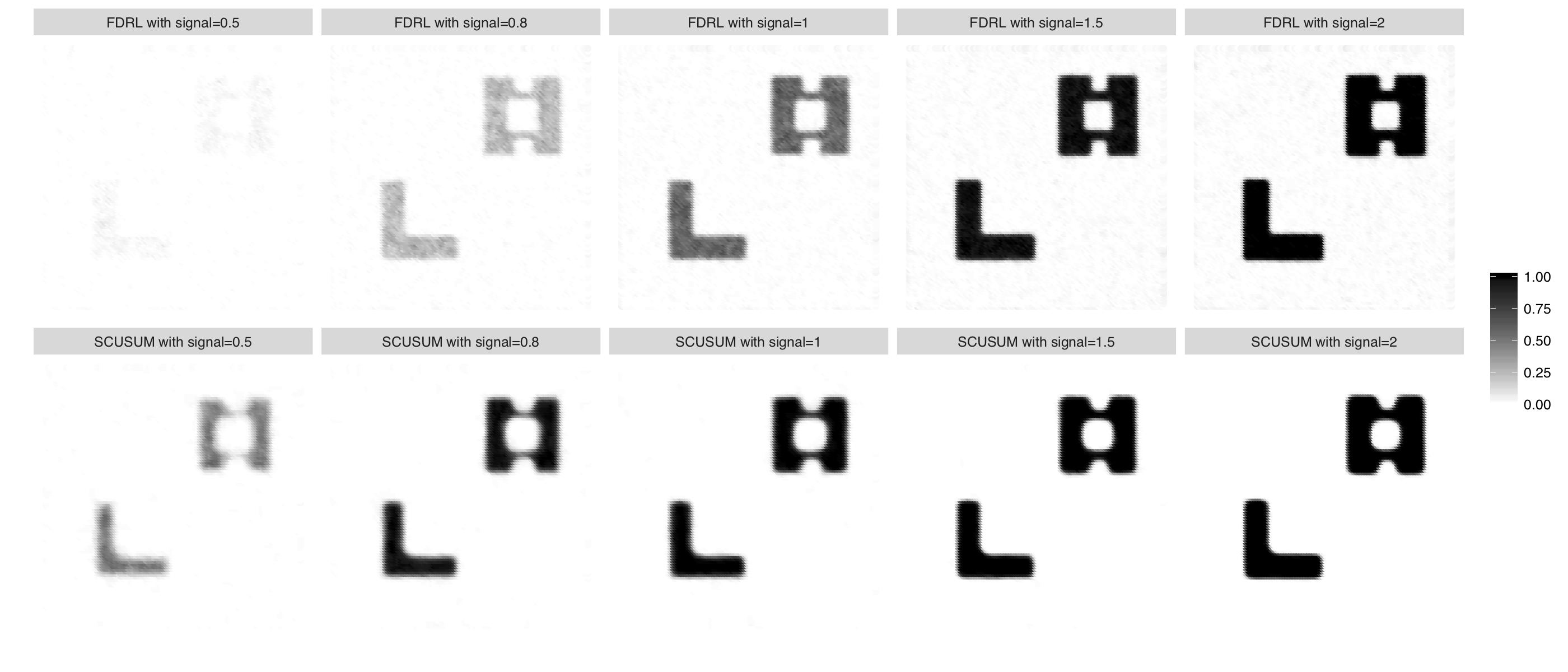
In Figure 6, we show the probability maps of the pixels being detected by the two methods with give . Here we set the neighbor size which we think has performance from Table 1 (relatively lower false positive and false negative). We range the signal strength from to In the probability maps, the darker the color is, the higher probability the corresponding point is signal. Comparing the probability maps with the ground truth (see Figure 5), it could be easily see that with hige signal strength the two methods have almost the same performance; while the signal is much too low (e.g.,) SCUSUM has a better detected result than FDRL. Also we can see that in the results of FDRL there are some shadows outside of ’L’ and ’H’ signal region, which are false positive; while for SCUSUM, the detections for indifference region are more ’white’ (no shadows.) To some degree, these probability maps are consistent with the experiment data in Tabel 1.
Though in model 2 we assume the noise to be independence, now we try to apply SCUSUM to dependence spatial observations, and compare with FDRL. Here we consider to use the Exponential Covariance Model (Gelfand et al. 2010) to generate dependence data. The covariance matrix is
| (13) |
where and are two locations, is the distance between the two location, and is the dependence scale. The larger means the stronger dependence. Then the data are generate from multivariate normal distribution with above covariance matrix and correponding mean, for and for We range scale from and the corresponding covariances for unit distance are We set the neighbor size for both two alogrithms and to control marginal FDR. The results are shown in Figure 7 and Tabel 2. It could be seen that with the weak dependence, SCUSUM could still detect the signal region efficiently while control the false posive. However for FDR the false negative increases significantly with stronger dependence (see Table 2). Also Table 2 shows that larger dependence scale leads to larger false positive, false negative and FDR for SCUSUM. This gives us a hint that for larger scale dependence noise we need to choose relatively larger blocks. Nevertheless, we can see that SCUSUM could recognize the signal region with higher probability than FDRL, when the noise dependence is weak.

| Dependence Scale | ||||
| false negative | SCUSUM | 0.2721 | 0.2820 | 0.3108 |
| FDRL | 0.5213 | 0.5879 | 0.7317 | |
| false positive | SCUSUM | 0.00095 | 0.00154 | 0.00418 |
| FDRL | 0.00499 | 0.00411 | 0.00280 | |
| FDR | SCUSUM | 0.0086 | 0.0141 | 0.0386 |
| FDRL | 0.0622 | 0.0604 | 0.0590 | |
5 Real Data Experiment
In this section, we apply four methods, SCUSUM, scan statistics, the conventional FDR and FDRL, to a real fMRI data to illustrate their differences in real data application. The fMRI data has been analyzed in some previous works (Maitra 2009; Zhang and Zhu 2012 etc.)
Figure 8 (a) shows six slices of the fMRI images in a total of 22 slices. Each individual image has pixels. All these images show activities in different regions by heat maps. The pixels’ values are the transformations of -values from a previous study, which should follow a standard normal distribution, and we only care about detection of the regions with positive values.
As for the conventional FDR, the lack of identification phenomenon happened, e.g. all the signals of the fifth slice in Figure 8 (b) are missed . Also without considering spatial correlation, for example in the first slice of Figure 8 (b), some detected ’signals’ are scattered around, which means that some of them might be false positive. Although FDRL could make full use of the neighbor information of spatially structured data and improve the detection efficiency, many weak signals are missed, e.g. in fifth slice and sixth slice of Figure 8 (c), many active regions are not detected. For scan statistics, even though almost all the ’hot’ pixels are detected, the ’signal’ regions are too large, which is doubtable.
Similar to the conclusion in Section 4, SCUSUM is more likely to detect weak signals compared with FDR methods. In all the six slices, the detected regions are larger and cover the regions detected by FDR methods. Meanwhile, within each slice, SCUSUM could identifiy several irregularly shaped clusters. We can see that the detected regions form natrual clusters, and they are the spatially grouped ’hot’ parts in the raw images. These results show that our proposed method might be more suitable for detection of irregular shaped and weak spatial signals.
| (a) | (b) | (c) | (d) | (e) |
 | ||||
 | ||||
 | ||||
 | ||||
 | ||||
 |
6 Conclusion
In this work, we proposed a spatial signal detection method, SCUSUM, which could accommodate the local spatial information. SCUSUM consists of two steps: firstly signal weights are estimated by moving window projecting and CUSUM cut-off; then a threshold is determined with given significant level to control marginal false discovery rate. Our simulation study shows that our method has a better performance compared to FDRL method. Empirically, SCUSUM tends to detect spatially gouped and weak signals, which are missed by the other two methods. Finally, our method is applied to a real fMRI data to illustrate its detection effectiveness.
In model 2, though our method doesn’t need to specify the distribution for noise process, the noise processes are assumed to be independent, and this is a strong assumption in spatial statistics. In the future work, it could be possible to consider a dependent noise process. In our simulation, the result shows that with weak spaital dependent noise process, SCUSUM could still maintain it effectiveness. Another key issue is to consider how to combine multi-source image data. So far, we only consider the observations are scalar and use moving window idea to project spatial observations to a sequence. However, this projecting method could be problematic when the observation of a spatial location is high-dimensional data or functional data.
References
- Abazajian and Kaplinghat [2012] Kevork N Abazajian and Manoj Kaplinghat. Detection of a gamma-ray source in the galactic center consistent with extended emission from dark matter annihilation and concentrated astrophysical emission. Physical Review D, 86(8):083511, 2012.
- Aue et al. [2009] Alexander Aue, Robertas Gabrys, Lajos Horváth, and Piotr Kokoszka. Estimation of a change-point in the mean function of functional data. Journal of Multivariate Analysis, 100(10):2254–2269, 2009.
- Benjamini and Hochberg [1995] Yoav Benjamini and Yosef Hochberg. Controlling the false discovery rate: a practical and powerful approach to multiple testing. Journal of the royal statistical society. Series B (Methodological), pages 289–300, 1995.
- Benjamini and Yekutieli [2001] Yoav Benjamini and Daniel Yekutieli. The control of the false discovery rate in multiple testing under dependency. Annals of statistics, pages 1165–1188, 2001.
- Blumensath et al. [2013] Thomas Blumensath, Saad Jbabdi, Matthew F Glasser, David C Van Essen, Kamil Ugurbil, Timothy EJ Behrens, and Stephen M Smith. Spatially constrained hierarchical parcellation of the brain with resting-state fmri. Neuroimage, 76:313–324, 2013.
- Breed [2011] David S Breed. Weather monitoring techniques, November 15 2011. US Patent 8,060,308.
- Cattaneo et al. [2017] Matias D Cattaneo, Michael Jansson, and Xinwei Ma. lpdensity: Local polynomial density estimation and inference. 2017.
- Chen [1999] Song Xi Chen. Beta kernel estimators for density functions. Computational Statistics & Data Analysis, 31(2):131–145, 1999.
- Cho et al. [2016] Haeran Cho et al. Change-point detection in panel data via double cusum statistic. Electronic Journal of Statistics, 10(2):2000–2038, 2016.
- Cowling and Hall [1996] Ann Cowling and Peter Hall. On pseudodata methods for removing boundary effects in kernel density estimation. Journal of the Royal Statistical Society. Series B (Methodological), pages 551–563, 1996.
- Craddock et al. [2012] R Cameron Craddock, G Andrew James, Paul E Holtzheimer, Xiaoping P Hu, and Helen S Mayberg. A whole brain fmri atlas generated via spatially constrained spectral clustering. Human brain mapping, 33(8):1914–1928, 2012.
- Gelfand et al. [2010] Alan E Gelfand, Peter Diggle, Peter Guttorp, and Montserrat Fuentes. Handbook of spatial statistics. CRC press, 2010.
- Genovese and Wasserman [2002] Christopher Genovese and Larry Wasserman. Operating characteristics and extensions of the false discovery rate procedure. Journal of the Royal Statistical Society: Series B (Statistical Methodology), 64(3):499–517, 2002.
- Genovese et al. [2002] Christopher R Genovese, Nicole A Lazar, and Thomas Nichols. Thresholding of statistical maps in functional neuroimaging using the false discovery rate. Neuroimage, 15(4):870–878, 2002.
- Gladders and Yee [2000] Michael D Gladders and HKC Yee. A new method for galaxy cluster detection. i. the algorithm. The Astronomical Journal, 120(4):2148, 2000.
- Glaz and Balakrishnan [2012] Joseph Glaz and Narayanaswamy Balakrishnan. Scan statistics and applications. Springer Science & Business Media, 2012.
- Glaz et al. [2001] Joseph Glaz, Joseph I Naus, Sylvan Wallenstein, Sylvan Wallenstein, and Joseph I Naus. Scan statistics. Springer, 2001.
- Glaz et al. [2009] Joseph Glaz, Vladimir Pozdnyakov, and Sylvan Wallenstein. Scan statistics: methods and applications. Springer Science & Business Media, 2009.
- Gromenko et al. [2017] Oleksandr Gromenko, Piotr Kokoszka, and Matthew Reimherr. Detection of change in the spatiotemporal mean function. Journal of the Royal Statistical Society: Series B (Statistical Methodology), 79(1):29–50, 2017.
- Grover-Kopec et al. [2005] Emily Grover-Kopec, Mika Kawano, Robert W Klaver, Benno Blumenthal, Pietro Ceccato, and Stephen J Connor. An online operational rainfall-monitoring resource for epidemic malaria early warning systems in africa. Malaria Journal, 4(1):6, 2005.
- Haas [1990] Timothy C Haas. Kriging and automated variogram modeling within a moving window. Atmospheric Environment. Part A. General Topics, 24(7):1759–1769, 1990.
- Hall et al. [1995] Peter Hall, Joel L Horowitz, and Bing-Yi Jing. On blocking rules for the bootstrap with dependent data. Biometrika, 82(3):561–574, 1995.
- Horváth and Hušková [2012] Lajos Horváth and Marie Hušková. Change-point detection in panel data. Journal of Time Series Analysis, 33(4):631–648, 2012.
- Jones and Foster [1996] MC Jones and PJ Foster. A simple nonnegative boundary correction method for kernel density estimation. Statistica Sinica, pages 1005–1013, 1996.
- Kulldorff [1999] Martin Kulldorff. Spatial scan statistics: models, calculations, and applications. In Scan statistics and applications, pages 303–322. Springer, 1999.
- Kulldorff and Nagarwalla [1995] Martin Kulldorff and Neville Nagarwalla. Spatial disease clusters: detection and inference. Statistics in medicine, 14(8):799–810, 1995.
- Maitra [2009] Ranjan Maitra. Assessing certainty of activation or inactivation in test–retest fmri studies. Neuroimage, 47(1):88–97, 2009.
- Miller et al. [2001] Christopher J Miller, Christopher Genovese, Robert C Nichol, Larry Wasserman, Andrew Connolly, Daniel Reichart, Andrew Hopkins, Jeff Schneider, and Andrew Moore. Controlling the false-discovery rate in astrophysical data analysis. The Astronomical Journal, 122(6):3492, 2001.
- Naus [1965] JL Naus. Clustering of random points in two dimensions. Biometrika, 52(1-2):263–266, 1965.
- Naus [1982] Joseph I Naus. Approximations for distributions of scan statistics. Journal of the American Statistical Association, 77(377):177–183, 1982.
- Páez et al. [2008] Antonio Páez, Fei Long, and Steven Farber. Moving window approaches for hedonic price estimation: an empirical comparison of modelling techniques. Urban Studies, 45(8):1565–1581, 2008.
- Priebe et al. [2005] Carey E Priebe, John M Conroy, David J Marchette, and Youngser Park. Scan statistics on enron graphs. Computational & Mathematical Organization Theory, 11(3):229–247, 2005.
- Shen et al. [2013] Xilin Shen, Fuyuze Tokoglu, Xenios Papademetris, and R Todd Constable. Groupwise whole-brain parcellation from resting-state fmri data for network node identification. Neuroimage, 82:403–415, 2013.
- Sun et al. [2015] Wenguang Sun, Brian J Reich, T Tony Cai, Michele Guindani, and Armin Schwartzman. False discovery control in large-scale spatial multiple testing. Journal of the Royal Statistical Society: Series B (Statistical Methodology), 77(1):59–83, 2015.
- Tango [2000] Toshiro Tango. A test for spatial disease clustering adjusted for multiple testing. Statistics in medicine, 19(2):191–204, 2000.
- Thomson and Connor [2001] Madeleine C Thomson and Stephen J Connor. The development of malaria early warning systems for africa. Trends in parasitology, 17(9):438–445, 2001.
- Wang et al. [2006] Jigang Wang, Predrag Neskovic, and Leon N Cooper. Neighborhood size selection in the k-nearest-neighbor rule using statistical confidence. Pattern Recognition, 39(3):417–423, 2006.
- Wang and Samworth [2018] Tengyao Wang and Richard J Samworth. High dimensional change point estimation via sparse projection. Journal of the Royal Statistical Society: Series B (Statistical Methodology), 80(1):57–83, 2018.
- Wheeler [2007] David C Wheeler. A comparison of spatial clustering and cluster detection techniques for childhood leukemia incidence in ohio, 1996–2003. International Journal of Health Geographics, 6(1):13, 2007.
- Zhang et al. [2011] Chunming Zhang, Jianqing Fan, and Tao Yu. Multiple testing via fdrl for large scale imaging data. Annals of statistics, 39(1):613, 2011.
- Zhang and Zhu [2012] Lingsong Zhang and Zhengyuan Zhu. Spatial multiresolution cluster detection method. arXiv preprint arXiv:1205.2106, 2012.
- Zhang et al. [2010] Zhenkui Zhang, Renato Assunção, and Martin Kulldorff. Spatial scan statistics adjusted for multiple clusters. Journal of Probability and Statistics, 2010, 2010.
Appendix A Proof for Lemma 1
Proof.
In assumed model 2, the noise processes are independent. Thus, in the th block, the sampled representative is independent with the rest observations, which implies and are independent, i.e. Also the representatives and pseudo block means between blocks are indpendent. These lead that and are indepedent.
Under the null hypothesis i.e. there is no signal and pseudo block mean sequence are i.i.d, as well as representative sequence . For the distribution of we have following:
Here is the one possible decreasing order for presents the set of all the possible orders. The first equation is according to bayesian formula; the second equation is because of under the independence of the third equation is due to independence between and the fourth equation is because are independent; the fifth equation is due to the cardinality of is From above result, we reach that are also i.i.d, having the same distribution with .
Under the alternative hypothesis as the number of observations in each block goes to infinity, the weak law of larger number supports that Thus, with (3) and (4), (5) holds. And is the number of block inside the signal region, is the number of block inside the indifference region and is the number of block at the boundary. ∎
Appendix B Proof for Theorem 1
Proof.
The proof idea is similar with [2]. W.l.o.g, here we consider the variance of noise processes is and Define the ratio of signal region to the entire spatial domain is hence, as blocks become finer and finer (), the ratio of the blocks with signal representative to the total blocks is getting closer to
Under define the following events:
| (14) |
Event presents the scenario that the order of is from signal blocks to interim (boundary) blocks and then to indifferent blocks (see Figure 3 (b).) And with Lemma 1, as
With event following we show that the probability of cut-off location falling into would converge to To proof that, we define statistics
| (15) |
First consider the probability of event with is a fixed constant. Define and note that is a constant.
where And with equation (5), following equations hold:
| (16) | ||||
| (17) |
Define the following statistics:
| (18) |
So and
As we have
the last equation is due to the reaches the maximum with Also we have
If we could prove is the leading term in then
Hence
Following lemmas support that is the leading term in with
Lemma 3.
With the assumptions of Theorem 1, given
| (19) |
Proof.
With the brief derivation, we have,
the last equation is because of
For
the last equation is due to the law of iterated logarithm and the weak law of large number. Similarly, for
Hence, with continuous mapping theorem, we have the result. ∎
Lemma 4.
With the assumptions of Theorem 1, given
| (20) |
Proof.
Lemma 5.
With the assumptions of Theorem 1, given
| (21) |
Proof.
The above three lemmas support that is the leading term in with Hence, the probability of event as and
For the other side, consider event with a given and Similarly define and following we will show asymptotically with probability
Define the following statistics:
| (23) |
Similarly, we have Also, as so we have
and
Following lemma shows that is the leading term in with
Lemma 6.
With the assumptions of Theorem 1, given we have
| (24) |
With above conclusion, we have
which implies
With these results, we have
as and
∎
Appendix C Proof for Lemma 2
Proof.
This lemma is easy to prove: from Lemma 1, as are i.i.d. Consider sequence then Note that in the left side equal to the reversed sequence Via applying CUSUM cut-off on and the detection result is opposite. Hence the distribution for signal weights under is symmetric under the asymptotical setting.
∎