First-order continuous- and discontinuous-Galerkin moment models for a linear kinetic equation: realizability-preserving splitting scheme and numerical analysisJournal: arXiv.org
Abstract
We derive a second-order realizability-preserving scheme for moment models for linear kinetic equations. We apply this scheme to the first-order continuous () and discontinuous () models in slab and three-dimensional geometry derived in [56] as well as the classical full-moment models. We provide extensive numerical analysis as well as our code to show that the new class of models can compete or even outperform the full-moment models in reasonable test cases.
Keywords:
moment models , minimum entropy , kinetic transport equation , continuous Galerkin , discontinuous Galerkin , realizability1 Introduction
We consider moment closures, which are a type of (non-linear) Galerkin projection, in the context of kinetic transport equations. Here, moments are defined by taking velocity- or phase-space averages with respect to some (truncated) basis of the velocity space. Unfortunately, the truncation inevitably comes at the cost that information is required from the basis elements which were removed.
The specification of this information, the so-called moment closure problem, distinguishes different moment methods. In the context of linear radiative transport, the standard spectral method is commonly referred to as the closure [36], where is the degree of the highest-order moments in the model. The method is powerful and simple to implement, but does not take into account the fact that the original function to be approximated, the kinetic density, must be non-negative. Thus, solutions can contain negative values for the local densities of particles, rendering the solution physically meaningless. Entropy-based moment closures, typically denoted by models in the context of radiative transport [41, 18], have (for physically relevant entropies) all the properties one would desire in a moment method, namely positivity of the underlying kinetic density, hyperbolicity of the closed system of equations, and entropy dissipation [35]. These models are usually comparatively expensive as they require the numerical solution of an optimization problem at every point on the space-time grid. Practical interest in such models increased recently due to their inherent parallelizability [25]. While the cost of solving the local nonlinear problems in the model scales strongly with the number of moments (since one has to solve square problems of size ), the desired spectral convergence with respect to the moment order is only achieved for smooth test cases, which rarely occur in reality. This means that the gain in efficiency by increasing the order of approximation will become rather insignificant.
To increase the accuracy of the models while maintaining the lower cost for small moment order , a partition of the velocity space while keeping the moment order fixed is useful, similar to some h-refinement for, e.g., finite element approximations [6]. We focus on the continuous and discontinuous piece-wise linear bases derived in [56], which aim to be a generalization of the special cases provided in [20, 19, 53, 44, 57] in slab geometry and the fully three-dimensional case.
Besides their inherent parallelizability, in order to make these methods truly competitive with more basic discretizations, the gains in efficiency that come from higher-order methods (in space and time) are necessary. Here the issue of realizability becomes a stumbling block. The property of positivity implies that the system of moment equations only evolves on the set of so-called realizable moments. Realizable moments are simply those moments associated with positive densities, and the set of these moments forms a convex cone which is a strict subset of all moment vectors. This property, even though desirable due to its consistency with the original kinetic distribution, can cause problems in numerical simulations. Standard high-order numerical solutions (in space and time) to the Euler equations, which indeed are an entropy-based moment closure, have been observed to have negative local densities and pressures [62]. Similar effects have been reported in the context of elastic flow [46]. This is exactly loss of realizability.
We propose a second-order realizability-preserving scheme, that is based on a splitting technique and analytic solutions of the stiff part, combined with a realizability-preserving reconstruction scheme. It turns out that this scheme is very effective for (medium) smooth and non-smooth test cases, which can also occur in practice. The realizability-preserving property is achieved using the realizability limiter proposed in [2, 54, 51, 15]. This limiter requires information about the set of realizable moments, which turns out to be very simple in the context of our first-order models [56]. Again, this additionally makes the implementation of such models faster (and easier) compared to standard models.
This paper is organized as follows. First, we shortly recall the transport equation, its moment approximations and the relevant results from [56] (Sections 2 and 3). Then, we propose our second-order realizability-preserving scheme and investigate all the required properties that it should fulfill (Section 4). In Section 5, we discuss some implementation details of our scheme. Finally, in Section 6, we give a comprehensive numerical investigation of our models and the models in slab geometry and three dimension, to show that our models can indeed compete with or even outperform the full-moment models.
2 Modeling
This section closely follows the corresponding part in [56]. We consider the linear transport equation
| (2.1a) | |||
| which describes the density of particles with speed at position and time under the events of scattering (proportional to ), absorption (proportional to ) and emission (proportional to ). Collisions are modeled using the BGK-type collision operator | |||
| (2.1b) | |||
| The collision kernel is assumed to be strictly positive, symmetric (i.e. ) and normalized to . In this paper, we restrict ourselves to isotropic scattering, where . | |||
The equation is supplemented with initial condition and Dirichlet boundary conditions:
| (2.1c) | |||||
| (2.1d) |
where is the outward unit normal vector in . Parameterizing in spherical coordinates we obtain
| (2.2) |
where is the azimuthal and the cosine of the polar angle.
Definition 2.1.
The vector of functions consisting of basis functions , of maximal order (in ) is called an angular basis.
The so-called moments of a given distribution function are then defined by
| (2.3) |
where the integration is performed component-wise.
Furthermore, the quantity is called the local particle density. Additionally, is called the isotropic moment.
Equations for can then be obtained by multiplying (2.1) with and integration over , resulting in
| (2.4) |
Depending on the choice of the terms , , , and in some cases even , cannot be given explicitly in terms of . Therefore an ansatz has to be made for closing the unknown terms. This is called the moment-closure problem.
In this paper the ansatz density is reconstructed from the moments by minimizing the entropy-functional
| (2.5) |
The kinetic entropy density is strictly convex and twice continuously differentiable and the minimum is simply taken over all functions such that is well defined. This problem, which must be solved over the space-time mesh, is typically solved through its strictly convex finite-dimensional dual,
| (2.6) |
where is the Legendre dual of . The first-order necessary conditions for the multipliers show that the solution to (2.5), if it exists, has the form
| (2.7) |
This approach is called the minimum-entropy closure [35]. The resulting model has many desirable properties: symmetric hyperbolicity, bounded eigenvalues of the directional flux Jacobian and the direct existence of an entropy-entropy flux pair (compare [35, 52]).
The kinetic entropy density can be chosen according to the physics being modelled. As in [35, 25], Maxwell-Boltzmann entropy
| (2.8) |
is used, thus . This entropy is used for non-interacting particles as in an ideal gas.
Substituting in (2.4) with yields a closed system of equations for :
| (2.9) |
Remark 2.2.
For convenience, we write (2.9) in the standard form of a non-linear hyperbolic system of partial differential equations:
| (2.11) |
where
| (2.12a) | ||||
| (2.12b) | ||||
For ease of visibility, we also consider our models in slab geometry, which is a projection of the sphere onto the -axis [58]. The transport equation under consideration then has the form
| (2.13) |
The shorthand notation then denotes integration over instead of . Finally, the moment system is given by
| (2.14) |
3 Angular bases
We shortly recall the angular bases under consideration. For a detailed derivation and further information, we refer the reader to [56] .
3.1 Slab geometry
- •
Full-moment basis
(3.1a) (3.1b) with the monomials or the Legendre polynomials , .
- •
Piecewise-linear angular basis (hat functions, continuous-Galerkin ansatz)
(3.2) where are some angular “grid” points and is the indicator function on the interval (with ).
- •
Partial moments (discontinuous-Galerkin ansatz)
where is the number of intervals.
3.2 Angular bases in three dimensions
Albeit both approaches are not limited to this, we consider moments on spherical triangles. To that end, let be a spherical triangulation of and be a spherical triangle. In this paper, the triangulation will be obtained by dyadic refinement of the octants of the sphere , i.e. the coarsest triangulation contains the eight spherical triangles obtained by projecting the octahedron with vertices , , to the sphere and finer partitions are obtained by iteratively subdividing each spherical triangle into four new ones, adding vertices at the midpoints of the triangle edges. After refinements, we thus obtain vertices and spherical triangles.
The bases that we use are the following.
- •
- •
- •
Partial moments on the unit sphere
where is the number of moments.
Naming of the models will be analogous to the slab-geometry case, compare Definition 3.1.
3.3 Realizability
The minimum-entropy moment problem (2.5) has a solution if and only if the moment vector is realizable.
Definition 3.2.
The realizable set is
If , then is called realizable. Any such that is called a representing density.
Unfortunately, checking whether a moment vector is realizable is not trivial for general bases. However, for the piecewise linear moment models, the realizability conditions are particularly simple (see [56]).
Lemma 3.3.
For the hat function basis in one or three dimensions, if and only if for all .
Lemma 3.4.
For the partial moment basis in one dimension (slab geometry), if and only if
| (3.3) |
for all .
For more details on the realizability of the regarded models, see [56].
4 Second-order realizability-preserving splitting scheme
As already mentioned before, the minimum-entropy moment problem (2.5) has a solution if and only if the moment vector is realizable. This implies that it is mandatory to maintain realizability during the numerical simulation (since otherwise the flux function cannot be evaluated). Explicit high-order schemes have been developed in [2, 54]. Unfortunately, the physical parameters and directly influence the CFL condition, resulting in very small time steps for large scattering/absorption.
This can be overcome by using a first-order implicit-explicit time stepping scheme [51, 48, 49], treating the transport part explicit while implicitly solving the (time-)critical source term. Unfortunately, using higher-order IMEX schemes again results in a CFL condition of the same magnitude as for the fully explicit schemes.
We are interested in a second-order scheme for (2.11). This can be achieved by doing a Strang splitting for
| (4.1a) | ||||
| (4.1b) | ||||
A second-order realizability preserving scheme will be obtained if both subsystems are solved with a (at least) second-order accurate and realizability-preserving scheme. For notational simplicity, we show the full scheme for one spatial dimension only. A generalization to structured meshes in higher dimensions is straightforward.
4.1 Source system
Let us start with the stiff part (4.1b) whose finite-volume form is given by
| (4.2) |
Fortunately, using the midpoint rule, it holds that
| (4.3) |
To obtain a second-order accurate solution of (4.2), it is thus sufficient to solve the system
| (4.4) |
which is purely an ODE (in every cell). As mentioned above, we restrict ourselves to isotropic scattering, where we have , i.e.
| (4.5) |
The source term now becomes
| (4.6) | ||||
where is the matrix mapping the moment vector to the isotropic moment vector with the same density . Here we assumed that there exists a vector such that (true for all regarded bases: for Legendre Polynomials, for real spherical harmonics, for the hat functions basis, for the partial moments in slab geometry and for the partial moment basis in three dimensions).
Since in this case, (4.4) is linear and the parameters , , are time-independent, we solve it explicitly using matrix exponentials, trivially obtaining a realizable second-order accurate solution of (4.2).
Remark 4.1.
Note that in this specific situation, the solution of this sub-step does not depend on the moment closure used in the flux system.
Using the matrix exponential and the variation of constants formula, the solution to (4.4) is
| (4.7) |
As and commute, we have
| (4.8) |
It remains to compute the matrix exponential of . As , we have that for all . It follows
| (4.9) |
Inserting (4.9) in (4.8), we get
| (4.10) |
Plugging (4.10) into (4.7), we finally get
| (4.11) | ||||
If the source is also isotropic then and (4.11) simplifies to
| (4.12) |
which can easily be calculated without explicit calculation of or any matrix operations.
4.2 Flux system
Let us now consider the non-stiff part (4.1a). This can be solved using standard realizability-preserving methods [54, 2, 52, 15], which will be summarized in the following.
The standard finite-volume scheme in semi-discrete form for (4.1a) looks like
| (4.13) |
where is a numerical flux function. The simplest example is the global Lax-Friedrichs flux
| (4.14) |
The numerical viscosity constant is taken as the global estimate of the absolute value of the largest eigenvalue of the Jacobian . In our case, the viscosity constant can be set to , because for the moment systems used here the largest eigenvalue is bounded in absolute value by one [2, 52, 42].
Another possible choice is the kinetic flux [54, 25, 22, 20]
| (4.15) |
where and denote integration over the positive and negative half intervals and , respectively. The kinetic flux is less diffusive than the (global) Lax-Friedrichs flux and admits a more consistent implementation of kinetic boundary conditions (see [52] and Section 5.5). For this reason, we will use (4.15) in all our computations.
4.2.1 Polynomial reconstruction
The value is the evaluation of a suitable linear reconstruction of at the cell interface . In one dimension, it can be obtained from a minmod reconstruction11 1 Other second-order accurate reconstructions like WENO [28, 16] are also possible.
where is the minmod function
applied componentwise. We then set and .
To avoid spurious oscillations, the reconstruction has to be performed in characteristic variables. They are found by transforming the moment vector using the matrix , whose columns hold the eigenvectors of the Jacobian evaluated at the cell mean . This leads to
| (4.16) |
For details on the eigenvalue computation see Section 5.2. In several dimension, we perform a dimension-by-dimension reconstruction as in [60] using the minmod reconstruction in characteristic variables in each one-dimensional reconstruction step.
4.2.2 Realizability-preservation
While this already gives us a second-order scheme, we do not have the realizability-preserving property yet. To achieve this, we need to apply a realizability limiter, ensuring that is point-wise realizable at the interface nodes . We follow the construction from [2].
We replace with the limited version
| (4.17) |
The limiter variable dampens the reconstruction from unlimited () to first-order (). Assuming that is realizable, there exists at least one (namely ) such that for every in the set of quadrature nodes (where is the closure of ). Since the realizable set is a convex cone, and by continuity, it is guaranteed that there exists a minimal satisfying this assumption. We are thus searching for the solution of the minimization problem
| (4.18) |
In practice, given some interface node , we search for the intersection of the line (wrt. ) with the boundary of the realizable set, check if the value is in and store it in the case that it is.
For the presented first-order moment models, the solution of the above limiter problem can often be computed explicitly (see Section 5.3 for more details).
4.2.3 Solving the optimization problem
For the minimum-entropy models, in each stage of the time stepping scheme for (4.1a), we have to solve the optimization problem (2.5) once in each cell (to compute the Jacobians) and twice at each interface of the computational mesh (one optimization problem for the left and right reconstructed value at the interface, respectively). This usually accounts for the majority of computation time which makes it mandatory to pay special attention to the implementation of the optimization algorithm. In this section, we will focus on the stopping criteria for the optimization algorithm. For details on the implementation, see Section 5.1.
Recall that the objective function in the dual problem (2.6) is
| (4.19) |
The gradient and Hessian of are given by
| (4.20) |
and
| (4.21) |
respectively. Note that since we assumed that (and thus also ) is strictly convex, and remember that the basis functions contained in are linearly independent. As a consequence, the Hessian is symmetric positive definite.
To find a minimizer of , we are searching for a root of the gradient using Newton’s method. For simplicity, we will restrict ourselves to Maxwell-Boltzmann entropy (2.8) such that . We use the Newton algorithm from [52, 2, 55] with some adaptions. Before entering the algorithm for the moment vector we rescale it to
| (4.22) |
such that . Let be the mapping which maps a set of multipliers to the density of its associated moment. If the optimization algorithm for stops at an iterate , we return
| (4.23) |
where is the multiplier with the property that (see Section 4.1). This ensures that the local particle density is preserved exactly:
| (4.24) |
Given , , we will stop the Newton iteration at iterate if
| (4.25a) | ||||
| (4.25b) | ||||
where is obtained from by (4.23) and, as always, is the number of moments.
In the following, we will explain the rationale behind these stopping criteria.
The first criterion guarantees that the gradient of the objective function is sufficiently small.
Lemma 4.2.
Let . If (4.25a) is fulfilled, we have that .
Proof.
First note that, by its definition (4.20), the gradient can be written as
| (4.26) |
where is the moment vector corresponding to the multipliers .
Let . Then it follows that
Consequently, we have
| (4.27) | ||||
Moreover,
| (4.28) | ||||
where in the last step we used the explicit forms of for the different bases (see Section 4.1). Since
| (4.29) |
it follows from (4.28) and (4.25a) that
for partial moments and hat functions, and
for full moments, which directly gives
respectively. Inserting these bounds in (4.27), we finally obtain
for partial moments and hat functions, and similarly for full moments, removing accordingly. ∎
The second criterion (4.25b) ensures that the ansatz density (2.7) corresponding to the multiplier obtained from the Newton iteration is close enough to a representing density for the moments .
Lemma 4.3.
Let and let , such that the second stopping criterion (4.25b) holds. Then there exists a representing distribution for , i.e. , such that
| (4.30) |
Proof.
In Section 4.2.4 we will use Lemma 4.3 to show that the scheme is realizability-preserving although the optimization problems are only solved approximately.
Remark 4.4.
Note that
is realizable for all . Due to the openness of , there exists a s.t. for all with . Note further that
so (4.25b) is fulfilled if , i.e. if our numerical solution to the approximation problem is close enough to the exact solution. For moments that are very close to the realizable boundary (so is very small and in addition may be very badly conditioned), we might not be able to achieve such an accuracy. In that case, we either use a regularized version of (see (5.6)) or disable linear reconstruction (see Item 4 in Section 5). Choosing closer to makes it easier to fulfil (4.25b) at the expense of smaller time steps (see Lemma 4.5). In our computations, we used the value which worked well in practice.
4.2.4 Time-step restriction
Now we are able to put all the things together to show that one forward-Euler step of our scheme (4.13) is indeed realizability-preserving.
Lemma 4.5.
Proof.
Adapted from [52, Theorem 3.19]. As we are using time stepping schemes that consist of a convex combination of Euler forward steps, it is enough to show realizability preservation in a single Euler forward step. Consider the one-dimensional () case first. The update formula in one step is
where is an arbitrary representing density for and is the ansatz distribution obtained from the approximate solution of the optimization problem. To preserve realizability, we have to ensure that for all and all cells .
For , after stripping away positive terms and using , we have
| (4.34) |
where is the distribution from (4.30).
We have that
| (4.35) |
where is the (limited) slope on cell . Thus we have
| (4.36) |
and therefore a representing density for is . Inserting this in (4.34) gives
| (4.37) |
This is positive under the time step restriction
| (4.38) |
The case follows in a similar way.
In dimensions, the update formula changes to
| (4.39) |
where is an index tuple. As in one dimension, we define the representing density and only regard the case , the other cases follow similarly. After stripping away positive terms we are left with
| (4.40) |
where . We proceed as in one dimension and note that
| (4.41) |
is a representing density for for any partition of unity . Inserting this ansatz in (4.40) gives
| (4.42) |
This is positive if
| (4.43) |
So for given we have to find a partition of unity such that the right-hand side of (4.43) is maximal, i.e., we want to find
| (4.44) |
Obviously, the maximum is attained if for all (otherwise we could increase the which belongs to the minimum and decrease the other ones a little). Taking the partition of unity property into account, we thus have to choose . Inserting this in (4.44) gives
5 Implementation details
We implemented the whole scheme in the generic C++ framework DUNE [8, 7], more specifically in the DUNE generic discretization toolbox dune-gdt [47] and the dune-xt-modules [39, 40].
As mentioned above, we advance the flux system in time using Heun’s method, which is a second-order strong-stability preserving Runge-Kutta scheme [23]. In each stage of the Runge-Kutta scheme, we perform the following steps:
- 1.
Solve the optimization problem for the cell means in each grid cell (see Section 5.1). If regularization is needed, replace by its regularized version22 2 This formally destroys the consistency of the scheme. However, since regularization rarely occurs (and only near the realizability boundary), this effect can usually be neglected in practice. (see Section 5.1.2).
- 2.
Reconstruct the values at the cell interfaces using linear reconstruction in characteristic variables (see Section 4.2.1), using the solution of the optimization problems from step 1 to calculate the Jacobians.
- 3.
Perform the realizability limiting (see Section 5.3).
- 4.
Solve the optimization problem for all reconstructed values . If the solver fails for a reconstructed value, disable the linear reconstruction in that cell.
- 5.
In the following, we will give some details on the implementation of these steps.
5.1 Implementation of the minimum-entropy solver
Our solver for the optimization problem is based on the algorithm from [3]. It uses a Newton-type algorithm with Armijo line search, i.e. to find a minimizer of the objective function (see (4.19)), we are searching for a root of the gradient (see (4.20)) in the Newton direction which solves
| (5.1) |
and then update the multipliers as
| (5.2) |
where is determined by a backtracking line search such that
| (5.3) |
with .
We stop the optimization if the new iterate satisfies the stopping criteria (4.25), except that we use
| (5.4) |
as the first stopping criterion instead of simply using (4.25a). This avoids numerical difficulties for moments with small density, where is in the order of and thus some iterates with very large (in absolute values) entries might fulfil the stopping criterion by chance. Moreover, checking the second stopping criterion (4.25b) might be quite expensive (depending on the basis ). We therefore check this criterion only if additionally
| (5.5) |
holds. This criterion approximately ensures (4.30) (see [52, 3]) but, in general, is much easier to evaluate than (4.25b). For the models, however, checking realizability is just checking positivity, so in that case we do not need to check (5.5) first.
To improve the performance and stability of the algorithm, we use several additional techniques which we will detail in the following. The values of the algorithms’ parameters that we use in all computations are given in Table 1.
| Newton algorithm | |||||||
|---|---|---|---|---|---|---|---|
| Realizability limiter | Minima | ||||||
5.1.1 Adaptive change of basis
Though the Hessian is positive definite and thus invertible, it may be very badly conditioned, especially for multipliers corresponding to moments close to the boundary of the realizable set. Moreover, in general, the integral in the definition (4.21) of can only be calculated approximately using a numerical quadrature (see Section 5.4). If the quadrature is not sufficiently accurate, the approximate Hessian may have a significantly worse condition or may even be numerically singular.
To improve this situation, a change of basis can be performed after each Newton iteration such that the Hessian at the current iterate becomes the unit matrix in the new basis [3]. We use this procedure in our implementation for all bases except for the hat function bases .
For the hat function basis, all matrices and vectors required in the optimization algorithm are sparse and exploiting this fact in the implementation greatly speeds up the computations. Including the change of basis destroys the sparsity and thus harms performance. In theory, this could be compensated by faster convergence and thus less iterations of the algorithm due to the condition improvements. Further, the algorithm with change of basis might use regularization less frequently and thus introduce less errors in the solution, as shown for the full moments in [3]. We thus compared the algorithm with and without change of basis in several test problems. The differences in the results were negligible in all tests cases and the version without change of basis was significantly faster. We thus do not use the adaptive change of basis for the hat functions.
The first-order partial moments have a similarly simple structure as the hat functions, so the adaptive change of basis might also not be needed for these models. However, the change of basis does not have a significant performance impact in this case as the support of each basis function is restricted to a single interval or spherical triangle, and thus all matrix operations can be performed on the or submatrices corresponding to an interval in 1d and a spherical triangle in 3d, respectively. Similar, quadrature evaluations can be performed for each interval or spherical triangle separately. For this reason, we include the adaptive change of basis in our optimization algorithm for the partial moments.
5.1.2 Regularization
For tests with strong absorption, the local particle density may become very small in parts of the domain. As a consequence, also the entries of the Hessian become very small which may cause numerical problems. We thus choose a “vacuum” density with corresponding local particle density . We then enforce a minimum local particle density of by replacing moments with local particle density by the isotropic moment with vacuum density . Obviously, this approach leads to a violation of the conservation properties of the scheme. However, since we only replace moments with very small local particle densities by moments with slightly larger but still very small densities, the effect should be negligible in practice.
Additionally, if the optimizer fails for a moment vector (for example, by reaching a maximum number of iterations or being unable to solve for the Newton direction) we use the isotropic-regularization technique from [3], i.e. we replace by the regularized moment vector
| (5.6) |
and retry the optimization. If the optimizer still fails, we increase until the optimizer succeeds, which is guaranteed at least for where is isotropic. As the regularized moment vector always has the same local particle density as the original moment vector , this technique does not violate the mass conservation of the scheme but it may potentially completely alter the solution. In practice, regularization is only used rarely and if it is used, a small regularization parameters is usually sufficient.
5.1.3 Caching
We use two types of caching. First, for each grid cell we store the moment vector from the last time step and the corresponding multiplier obtained by entropy minimization. In this way we do not have to solve the optimization problem again if the moment vector in that grid cell did not change during the last time step. In addition, we store the last few solutions of the minimization problem with corresponding input moment vectors per thread of execution, so if several grid cells contain the same values, we only have to perform the optimization once and then use the cached values. If we encounter a moment vector that can not be found in the caches, we take the moment vector that is closest to the input vector (in one-norm) and use the corresponding multiplier as an initial guess.
5.1.4 Linear solvers
In each iteration of the Newton scheme, we have to apply the inverse of a positive definite Hessian matrix. We assemble the matrices using the quadratures described in Section 5.4. Inversion is then done by computing a Cholesky factorization of the assembled matrix. For the full moment models, the Hessian matrices are dense, so we use the LAPACK [5] routine dpotrf to compute the factorization and then use dtrsv to actually invert the linear systems. For the models, the Hessian is block-diagonal (each block corresponds to one interval/triangle of the partition) such that we can perform the Cholesky decomposition independently for each block. For the models in one dimension, the Hessian matrices are tridiagonal, so we can use the specialized LAPACK algorithms dpttrf and dpttrs. In three dimensions, the Hessians are not tridiagonal anymore but still sparse, so we use the sparse SimplicialLDLT solver from the Eigen library [24].
5.2 Solving the eigenvalue problems
To avoid spurious oscillations, the reconstruction has to be performed in characteristic coordinates (see Section 4.2.1). For that reason, we have to compute the eigenvectors of the flux Jacobians
| (5.7) |
where
| (5.8) |
and
| (5.9) |
(compare Section 4.2.3). Note that, in general, the Jacobian (5.7) is not symmetric. However, since is symmetric and symmetric positive definite (see Section 4.2.3), we can see that is similar to a symmetric matrix, i.e.
and thus has real eigenvalues. In our implementation, we explicitly compute the matrix representation and then use an eigensolver for non-symmetric matrices (LAPACK’s dgeevx) to obtain the eigen decomposition. Unfortunately, though the Jacobian is a real matrix with real eigen values and thus also admits a set of real eigenvectors, the standard solvers for non-symmetric eigen problems (apart from dgeevx, we also tested the EigenSolver of the Eigen library [24]) often return complex eigenvectors. We thus add a step to compute real eigenvectors from the complex ones. Note that if
| (5.10) |
is a set of linearly independent complex eigenvectors to the same eigenvalue for the Jacobian , where is the imaginary unit and are real vectors, then
| (5.11) |
is a set of real eigenvectors for . Moreover, there are at least linearly independent vectors in this set. To see that, assume the opposite, i.e. that any vectors from the set (5.11) are linearly dependent. Without loss of generality, we assume that every vector in (5.11) can be written as a linear combination of the first vectors, i.e.
| (5.12) |
with coefficients . Then, the vectors can also be written as (complex) linear combinations of these real vectors
| (5.13) |
and thus cannot be linearly independent.
Consequently, to get real eigenvectors for from the complex ones computed by the eigensolver, we first sort the eigenvectors into sets belonging to the same eigenvalue and then perform a Gram-Schmidt process with the real and imaginary parts for each of these sets.
Remark 5.1.
While this procedure works reasonably well, a better approach would probably be to use the structure of the Jacobian and, instead of solving the non-symmetric eigenvalue problem
| (5.14) |
solve the symmetric generalized eigenvalue problem [37, 12]
| (5.15) |
and then get the eigenvectors as . Since the matrices and are both symmetric and is positive definite, we can use a specialized algorithm like LAPACK’s dsygv and directly obtain real eigenvectors. Moreover, we can take advantage of the sparsity of these matrices and, e.g., use a generalized eigenvalue algorithm aimed at band matrices like dsbgv. In contrast, explicit assembly of the term might destroy the structure and result in a dense matrix even if the two factor matrices are sparse.
For the partial-moment models, the eigen decomposition can be done block-wise on the or matrix blocks which reduces the cubic complexity of the eigen decomposition [43] to a linear complexity for increasing number of moments and thus greatly accelerates computations for large problems.
5.3 Realizability limiting
The linear reconstruction process in the finite volume scheme does not guarantee preservation of realizability. Thus, we need an additional limiting step (4.17) to ensure that we are able to solve the optimization problem (2.5) for the reconstructed values. Since, in general, we cannot solve the integrals occurring in the optimization problem analytically and have to approximate them by a numerical quadrature , the admissible moment vectors are further restricted to the numerically realizable set (-realizable set)
| (5.16) |
where for an integrable function , is the approximation of the corresponding integral with the quadrature rule . In general, the numerically realizable set is a strict subset of the analytically realizable set.
The numerically realizable set can be described as the convex hull of the basis function values at the quadrature nodes (see [3] for the Legendre basis, the proof can be easily adapted for the other bases)
| (5.17) |
If depends linearly on it follows
| (5.18) |
We do not want the limited moments to be too close to to the boundary of the numerically realizable set as we are not able to solve the optimization problem (2.5) in that case (see [4]). Moving the limited value away from the boundary can be done in several ways. A simple but often sufficient method can be employed for all limiters presented in this section. We simply add a small parameter to the final limiter variable [52]. A problem with this approach is that the connecting line between and might be almost parallel to the boundary which possibly results in a limited moment that is still too close to the boundary. Another approach is to require a fixed distance to the boundary of , i.e., to limit to the -realizable set
| (5.19) |
where is the Euclidian distance to . Limiting to this set is possible whenever is farther than away from the boundary. If is already in the -range of the boundary, we disable reconstruction in that cell.
Unfortunately, checking whether a reconstructed value lies within the numerically realizable set is not trivial in general. In the following, we detail the limiting procedure for the different models. For the remainder of this section, let be the moment vector before reconstruction and a reconstructed moment vector 33 3 In one dimension, there are always two reconstructed values per grid cell (one at each interface), so each of the limiters described in the following is applied to both values and the larger is used in (4.17). In several dimensions, both reconstruction and limiting are performed independently for each coordinate direction.. Let further and be the -th component of and , respectively.
5.3.1 models
In [2, 52], the half space representation for the convex hull (5.18) was explicitly calculated before starting the time stepping, yielding
| (5.20) |
where is the number of facets of the convex hull. During the time stepping, the intersection of the connecting line between and and each facet can then be computed efficiently by solving
(compare (4.17)) for the limiter variable. We thus obtain
| (5.21) |
If or , the moments can simply be rescaled before applying the limiter [2, 52]. Alternatively, we can ignore the facet corresponding to the condition which gives the half-space description for the full numerically realizable set (5.17). In that case, no rescaling is necessary and we can easily ensure a minimum distance of to the realizable boundary by moving each facet in normal direction before calculating the intersections, resulting in
| (5.22) |
instead of in (5.21). As for the other limiters, we disable reconstruction if does not lie within the -realizable set, i.e. if
| (5.23) |
However, explicit calculation of the convex hull is only viable for a relatively small number of moments (such that the convex hull has to be calculated in a low-dimensional space) or very sparse quadratures (such that the convex hull has to be calculated from a small number of points). For a larger number of moments and a reasonable fine quadrature, the construction of the convex hull takes excessively long. Moreover, even when the convex hull is available, the performance of this approach might be unacceptable as the number of facets grows rapidly with both the number of moments and the number of quadrature points [52]. We thus use this approach only for the partial moments (see Section 5.3.3) where we only have to calculate low-dimensional convex hulls.
For the models, as proposed in [52, Section 3.62], we instead utilize the quadrature description (5.16) of the numerically realizable set and limit by solving the linear program (LP)
| (5.24a) | |||
| (5.24b) | |||
| (5.24c) | |||
where should not be confused with but rather represents for the sought representing distribution . This approach removes the prohibitively costly explicit calculation of the convex hull. However, the runtime cost during the time stepping algorithm might be considerably higher as a linear program has to be solved for every reconstructed value.
Instead of using a single limiter variable , principally, we can limit each component of independently. This has been done, e.g., in the context of the Euler equations in [62]. However, if the limiting is naively performed in ordinary coordinates, spurious oscillations may occur, as the limiting in ordinary coordinates may actually increase the slope in one of the characteristic components. In our implementation, we thus limit each of the characteristic components independently. Let be the matrix of eigenvectors of the Jacobian and let , be the respective moment vectors in characteristic coordinates. Then we can find limiter variables for each characteristic component by solving the LP
| (5.25) |
where the matrix is defined as and the -th column of is .
For the LP-based limiter, it is not clear how to ensure a fixed distance to the boundary. We thus use the method of adding a small parameter to the final limiter variable by replacing by in (5.24c) and using instead of if it is in the interval .
For checking realizability of , which is needed for the stopping criterion (4.25b) in the optimization algorithm, we solve the simpler LP
| (5.26a) | |||
| (5.26b) | |||
| (5.26c) | |||
Note that the limiters presented thus far are not restricted to the models but could be used for any basis . However, for the and models, due to the simpler realizability conditions, limiters that are both faster and easier to implement can be used.
5.3.2 models
For the hat functions the numerically realizable set and the realizable set agree for suitable quadratures [56]. As a consequence, we can use a limiter based on the analytical realizability conditions which only require component-wise positivity (see Section 3.3). We thus calculate the limiter variable (limiting to as
| (5.27) |
5.3.3 models
In one dimension, for suitable quadratures, so a limiter based on the analytical realizability conditions (3.3) can be used. We use a limiter variable per interval . If we require a distance of at least to the boundary, the realizability conditions (3.3) become
| (5.28) |
If is already not -realizable, we disable reconstruction for that interval. This results in the following limiter for one-dimensional partial moments
| (5.29) |
where
For the partial moment basis in three dimensions, the analytical and numerical realizable set differ. However, note that (5.18) holds separately for each spherical triangle (see [56, Lemma 5.13]), so we can explicitly calculate the half space representation (5.20) for each spherical triangle. Instead of calculating a convex hull in dimensions, as would be needed for the full moment models, we only have to calculate convex hulls in dimensions, which is considerably faster and usually finished within a few seconds in our implementation (remember that this calculation has to be done only once before the time stepping).
5.4 Implementation of quadrature rules
In one dimension, we use Gauss-Lobatto quadratures on each interval. These quadratures include the endpoints of the interval, which ensures that the numerically realizable set (see (5.16)) equals the analytically realizable set for hat functions and partial moments, see [56]. To choose a suitable quadrature order, we solved some of our numerical test cases for different quadrature orders and calculated the errors with respect to the reference solution (see Section S2 in the supplementary materials). As suggested by this analysis, for the first-order models, we use a quadrature of order 15 per interval of the partition . For the full moment models, we split the domain in the two intervals and that are needed for calculation of the kinetic flux and use a quadrature of order on each interval.
In three dimensions, for partial moments and hatfunctions, we are using Fekete quadratures [59] (from the TRIANGLE_FEKETE_RULE library [13]) mapped to the spherical triangles. The library provides seven Fekete quadratures of order , , , , , and , using , , , , , , quadrature points, respectively. The second rule of order contains some negative quadrature weights, so we do not use that quadrature. If we want to improve the approximation, we subdivide each spherical triangle in several smaller ones as in [10] and use the mapped Fekete quadrature on each subtriangle. The Fekete rules correspond to Gauss-Lobatto rules on the triangle edges and thus also include the vertices of each triangle [59], which simplifies the realizability preservation (see [56]). As suggested by our quadrature sensitivity analysis (see Section S2), we use a quadrature order of for the and models and a quadrature order of for the other and models. For the models, we use tensor-product quadrature rules of order on the octants of the sphere.
For the hat function basis in one dimension, we alternatively explicitly calculate all integrals needed in the Newton algorithm using the analytical formulas and Taylor expansion at the numerical singularities of the analytical formulas (see [32, Appendix A1] for the explicit formulas). The Taylor expansion is performed in a neighborhood of radius around the singularity, up to vanishing remainder or a maximal order of . This completely removes the need for quadrature rules. Note that the same approach could be used for the partial moments in one dimension. However, as the quadrature-based adaptive-change-of-basis algorithm is very efficient for partial moments, we did not implement the analytical formulas for partial moments.
For the hat function basis in three dimensions, integrals cannot be evaluated analytically anymore. We experimented with an approach where the integrals are expanded in a Taylor series representation (see Section S1 in the supplementary materials). However, it turned out that the Taylor series had to be computed up to a prohibitively high order. For this reason, we dismissed that approach and use the Fekete quadrature approach described above also for the hat functions in three dimensions.
5.5 Implementation of initial and boundary conditions
The initial values for the finite volume scheme are computed by integration of the kinetic equation’s initial values (2.1c).
Since the initial values in our test cases are isotropic (see Section 6), i.e. , we only have to compute the velocity integral of the basis . For this integral, we use the same quadratures as in Section 5.4 to ensure that the result is numerically realizable. Except for the plane-source and point-source tests, the initial values are constant in each grid cell, so we use the midpoint quadrature to evaluate the spatial integral. For the plane-source test, we always use an even number of grid cells and distribute the Dirac delta at into the two adjacent grid cells, i.e. the initial value in these grid cells is set to the constant . For the point-source test, we use a Gauss-Legendre tensor product quadrature of order 20 to evaluate the spatial integrals for the initial values.
6 Numerical results
We want to apply our moment models to several test cases in the one- and three-dimensional setting. We follow the FAIR guiding principles for scientific research [61] and publish the code that generates the following results in [34]. As already mentioned (see Section 5), the scheme was implemented in the DUNE generic discretization toolbox dune-gdt [47]. The computations were done on a varying number of nodes of a distributed memory computer cluster44 4 Each node encloses two Intel Intel Skylake Xeon Gold 6140 CPUs ( cores) and GB RAM.. Communication between nodes was done via MPI (Message Passing Interface) [38]. On each node, we used a work-stealing task-based shared-memory parallelization which was implemented using Intel TBB [27].
6.1 Slab geometry (1D)
6.1.1 Plane source
In this test case an isotropic distribution with all mass concentrated in the middle of an infinite domain is defined as initial condition, i.e.
where the small parameter is used to approximate a vacuum. In practice, a bounded domain must be used which is large enough that the boundary should have only negligible effects on the solution. For the final time , the domain is set to (recall that for all presented models the maximal speed of propagation is bounded in absolute value by one).
At the boundary the vacuum approximation
is used again. Furthermore, the physical coefficients are set to , and .
All solutions are computed with an even number of cells, so the initial Dirac delta lies on a cell boundary. Therefore it is approximated by splitting it into the cells immediately to the left and right. In all figures below, only positive are shown since the solutions are always symmetric around .
Note that since the method of moments is indeed a type of spectral method, it can be expected that due to the non-smoothness of the initial condition the convergence towards the kinetic solution of this test case is slow (note that for any ). Nevertheless, it is an often-used benchmark revealing many properties of a moment model (see e.g. [22]).
Some exemplary solutions at the final time are shown in Figures 1, 2 and 3. Remember that the full-moment models are indexed by the basis order while the piecewise linear bases are indexed by the number of moments . Since, in one dimension, a basis of the space of polynomials up to order has elements, we compare the and models to the piecewise linear models with moments.
As expected, there are strong oscillations about the reference solution (the analytical solution from [21]) for all tested models. With increasing number of moments, the number of peaks increases while their height decreases. The oscillations are considerably stronger for the linear models than for the corresponding minimum-entropy models. The models are closest to the reference solution, particularly for the low-order models.
This is also reflected in the convergence results, which can be found in Figure 4. Depicted are the and errors between the local particle densities of the moment models and the analytic reference solution from [21] at the final time . As expected, overall convergence is slow. The , and models show very similar errors at all orders. With respect to norm, the models are slightly better than the models. As observed before for the models [50, 52], models with odd show a higher error than models with even due to a zero eigenvalue of the flux jacobian. A similar but much less pronounced behaviour can be seen for the models (for odd and even number of intervals ). For odd , errors are close to the corresponding error. For even the models perform better than the models and similar to the model.
The entropy-based , and models show lower errors than their linear counterparts both in and norm. The models perform slightly better than models of the same order. The difference between odd and even orders/number of intervals is much more pronounced than for the and models. The models give the lowest errors of all tested models. However, the errors are still high and the rate of convergence is equally bad for all models although the convergence rate seems to improve with higher orders, especially for the minimum-entropy-based models.
6.1.2 Source beam
The discontinuous version of the source-beam problem from [26] is presented. The spatial domain is , and
with initial and boundary conditions
The final time is and the same vacuum approximation as in the plane-source problem is used.
Convergence results can be found in Figure 5. The reference solution for this test case is computed from a direct finite difference discretization of the kinetic equation on a grid with elements. As expected due to the higher regularity of the test case55 5 is “only” a discontinuous function compared the distributional setting in the plane-source test., the convergence for all tested models is much better than in the plane-source test. As a consequence, most of the models are relatively close to the reference solution which is why we do not show exemplary solutions plots. The piecewise linear models and the models converge with second and first order in and norm, respectively. The models show spectral convergence which is reflected in comparatively high errors and a slow rate of convergence for the lower-order models and then a rapid convergence for the high-order models. Despite the eventual high rate of convergence, for the maximal moment number regarded here the models are mostly outperformed by the other models. Again, the minimum-entropy-based models perform better than their linear counterparts although the rate of convergence is the same. In norm, the , partial-moment and models again show a zig-zag pattern where, e.g., the models using an odd number of intervals (even number of moments ) perform better than the ones using an even interval number (odd ). For the partial-moment models, an even number of intervals gives better results. Notably, the do not show such an alternating behaviour.
6.2 Three dimensions
We now consider numerical results in three spatial dimensions with velocities on the unit sphere.
6.2.1 Point source
The point-source test is the three-dimensional analogue of the plane-source test (Section 6.1.1) in slab geometry. Due to the limitations in the resolution we use a smoothed version of the initial Dirac delta:
where , . As before, we choose , and . All models are calculated on to the final time . The grid size is chosen to be The point-source test is well-suited to demonstrate symmetries (or symmetry breaks) appearing in the solution. We show some selected models in Figures 6 and 7, where we use the endcap geometry for the isosurfaces.
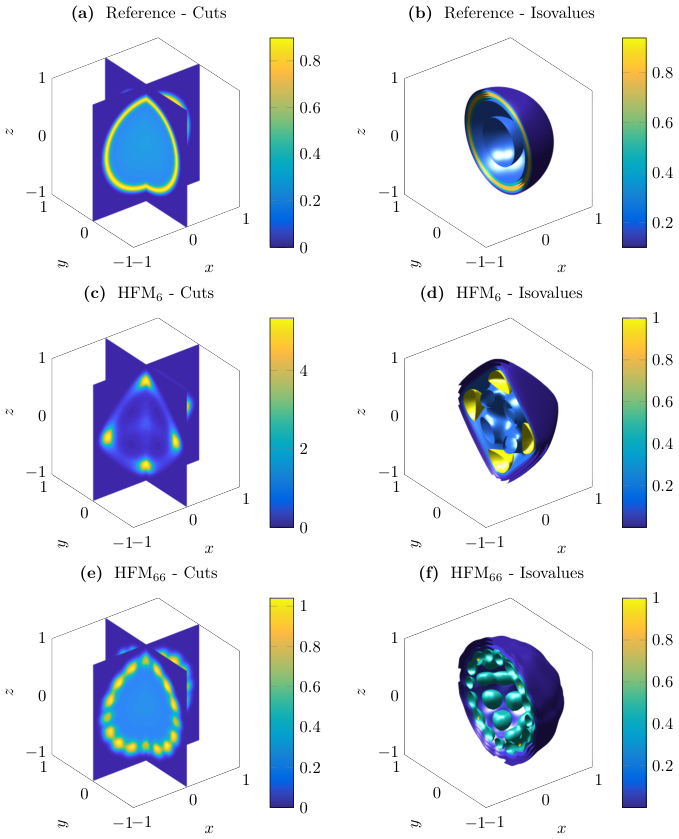
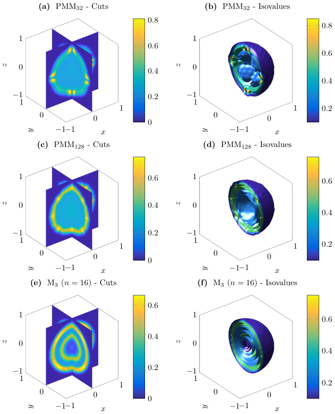
The reference solution itself is rotationally symmetric and can be computed analytically using the formulas by Ganapol [21]. It can be observed that the hat functions have a preferred directions of propagation, directly related to the position of the vertices in the spherical triangulation (e.g., the octahedron that defines the basis can be easily identified in Figure 6). Similar effects occur for the partial moments. However, the discontinuity of their basis is also reflected in the peaks along the boundaries of the spherical triangles (compare ). In contrast to this, the full-moment models preserve the rotational symmetry (compare , where small irregularities in the solution arise due to the spherical quadrature rule) but adding more waves to the solution.
Finally, we show error plots for our models in Figure 8. The models show the expected slow convergence in the -norm, similar to the plane-source test (Section 6.1.1). All first-order models show roughly order , whereas the full-moment models have varying convergence rates. In the -norm, the first-order models show order convergence in the beginning, which then slows down to order as well. The full-moment models are showing no (or very slow) convergence, which is the well-known Gibbs phenomenon.
Note that the models clearly outperform the other methods. In particular, they are as good as or even slightly better than the models whose calculation is significantly more expensive for the same degrees of freedom (see Section 6.3).
6.2.2 Checkerboard
The checkerboard test case is a lattice problem which is loosely based on a part of a reactor core [11]. We extend it in a straightforward manner to the three-dimensional case. The used geometry is shown in Figure 9. There are scattering (orange and green) and highly absorbing (black) regions. The parameters are chosen to be the following.
- •
Domain: , subdivided into the three regimes
- •
Final time: ,
- •
Parameters (compare Figure 9):
- •
Initial condition: (approx. vacuum),
- •
Boundary conditions: .
Due to the discontinuous nature of the physical parameters, this test case is a challenging task for a numerical solver. We align our grid with the discontinuities of the parameters by using a multiple of (usually ) regularly spaced grid points in each direction.
Solution plots for selected models can be found in the supplementary materials (Figures S3.1–S3.3). The model and the models of order (only shown) have negative particle densities . Surprisingly, the hat function basis has positive densities for all that we calculated.
We compare our models to a discrete ordinate implementation [31, 22] of second order. - and -errors of the local particle density can be found in Figure 10. All tested models converge with about first order both in and norm. Again, and models are comparable to the models.
6.2.3 Shadow
The shadow test case represents a particle stream that is partially blocked by an absorber, resulting in a shadowed region behind the absorber. The used geometry is shown in Figure 11.
The parameters are chosen to be the following.
- •
Domain:
- •
Final time: ,
- •
Parameters:
- •
Initial condition: (approx. vacuum),
- •
The isotropic particle stream with density enters the region via the boundary condition at . At all other boundaries, vacuum boundary conditions are used.
We show slices and isovalues of several models at the final time in the supplementary materials (Figures S.4–S.6). Again, several of the linear models (e.g. or ) show negative values (depicted in red). As in the previous test case, the partial moments perform very well. Compare, for example, the linear model to (which has roughly the same number of degrees of freedom). The partial-moment model approximates the reference much better, especially in the far field where also the small oscillations are captured accurately. A similar tendency can be observed for the hat function model .
Both hat function and discontinuous minimum-entropy models show a good approximation of the absorber (compare and ). However, they are not able to provide a reasonable approximation in the far field. Further repartitioning of the sphere yields much better results in this case.
Investigating again the convergence towards the reference solution (see Figure 12), we see that the full-moment models are slightly superior in the beginning, but convergence slows down for higher . Both as well as show a similar convergence behaviour. Again, taking running time into account, both models outperform the classical model in terms of efficiency (see Section 6.3). Note that we only computed models up to a order of since the higher-order models did not finish in the available computation time. The same is true for the models with . Distributing the workload among more nodes of the distributed cluster did not improve computation times for these models, which is probably due to load-balancing issues. While the task-stealing algorithm (see above) ensures that the work is distributed evenly on each node, there is no load-balancing between nodes. In our implementation, the grid is distributed to the nodes using a decomposition of the domain in connected parts. Since the optimization problems are particularly challenging near the absorber (due to low particle densities and very anisotropic distributions), the node(s) containing the absorber often need much longer than the other nodes to solve the optimization problems. Here, an MPI-based load-balancing implementation may be required which would, however, significantly increase the communication overhead. As an alternative, in [33], we investigate a numerical scheme that avoids the non-linear optimization problems and thus does not show the same load-balancing issues.
In conclusion, moment models based on piecewise first-order continuous (, ) or discontinuous (, ) basis functions often approximate the true solution as good as or even better than the standard models (, ) using polynomial bases. In contrast to the standard models, however, these models can be implemented very efficiently. This is especially true for the entropy-based models since the necessary realizability limiting can be based on the analytical realizability conditions (see Section 5.4). In addition, in case of the discontinuous models, all matrix operations can be performed on small matrix blocks which provides further performance advantages (also for the models, see Section 6.3).
6.3 Timings
Performance measurements can be found in Figure 13. The times were measured without parallelization. Displayed times are the minimum of three runs. Quadratures were chosen as described in Section 5.4. Measurements were done both for the first-order scheme without linear reconstruction and for the realizability-preserving second-order scheme (see Section 4). Profiling shows that the first-order scheme spends most of the time solving the optimization problems. For the second-order scheme, solving the eigen problems for the reconstruction in characteristic coordinates also has a large impact on the execution time. Here, computation times could probably be improved by using a generalized eigen solver which takes the structure of the Jacobians into account (see Section 5.2). Both the adaptive-change-of-basis scheme and the eigensolver have third-order complexity. We thus asymptotically expect third-order complexity in for both the first-order and the second-order scheme for the models. For the models, all operations (including the solution of the eigen problems) can be done block-wise, so we expect first-order complexity in that case. Regarding only the optimization problem, the same is true for models as all matrices involved are tridiagonal (in slab geometry) or very sparse (in three dimensions). However, the Jacobian of the flux function is not sparse in general for the models, so the eigen problems are currently solved with a standard third-order-complex eigensolver. These models would particularly benefit from an improved implementation of the eigensolver which exploits the fact that the Jacobians are products of two sparse symmetric matrices (see Section 5.2).
In slab geometry, we used a reduced version of the plane-source test case ( grid cells, final time ). For the models, two different implementations were tested: the backtracking Newton solver without change of basis (see Section 5.1.1) using quadratures to calculate the integrals and the same backtracking Newton solver where all needed integrals were solved using the analytical formulas (and Taylor expansion at the singularities, see Section 5.4). In three dimensions, we used a reduced version of the point-source test case ( grid cells, single Runge-Kutta step).
As can be seen in Figure 13, for the first-order scheme, results are as expected except that the models show second-order complexity in slab geometry, probably because the matrices are relatively small here and thus the third-order matrix operations do not dominate the execution time. The implementation using analytic integrals is faster than the quadrature version but the difference is negligible in practice. Given that the implementation using analytic integrals is considerably more complex and that analytic realizability conditions can also be used for the quadrature-based version, we suggest to generally use a quadrature-based implementation also for the models.
For the second-order scheme, as expected, the models show first-order complexity both in slab geometry and in three dimension and thus are several orders of magnitudes faster than the other models. Curiously, the models are close to second-order complexity also in three dimensions. For even larger , we expect the models to also increase with third-order due to the eigensolver but the results show that the models are much faster than the models for a long time.
Note that though the and models are equivalent, the measured times are different as the model uses the convex-hull based realizability limiter while the model uses the limiter based on the analytical realizability conditions to be consistent with the models with higher .
7 Conclusions and outlook
We derived two classes of minimum-entropy moment models based on a continuous finite element basis as well as a discontinuous piece-wise linear basis. Both types of models are realizable, i.e., generated by a non-negative ansatz, such that important physical properties like positivity of mass are preserved. We demonstrated in various numerical tests in one and three dimensional geometry that those models are qualitatively competitive with the classical full-moment models of the same number of degrees of freedom if the solution of the kinetic equation only has a limited smoothness (since otherwise the models typically show spectral convergence). Additionally, the new models are much cheaper (with respect to running time) than the full moment models since the non-linear problems that have to be solved locally are much smaller and typically much easier to solve as well. Consequently, the new models are considerably more efficient in the sense that they reach the same approximation error with much less computation effort. In particular, the partial moments show a linear relation between wall time and number of moments, which is also true for the hat function basis if only a first-order scheme is used. If a higher-order discretization in space and time is required, the partial moments appear to be the model of choice. However, in some cases the discontinuity in the basis functions may lead to severe problems, for example when collision is modeled with the Laplace-Beltrami operator [53]. In such cases, might be favorable.
We provided a second-order realizability-preserving scheme by using a splitting technique and analytic solutions of the stiff part, combined with a realizability-preserving reconstruction scheme. Higher-order variants of this scheme can in principle be derived similarly, but we emphasize that we strictly focused on non-smooth problems, where the sense in applying schemes with (much) more than second order is questionable.
If the underlying problem admits more smoothness (especially in the velocity domain), higher-order moment models might be more appropriate to enhance the speed of convergence towards the kinetic solution. While this is rather straight-forward to define both in slab as well as three-dimensional geometry (partial moments can be constructed immediately while the hat-function basis can be extended to higher-order splines on the unit interval/unit sphere,respectively [1]), special care is required since the realizability conditions are needed in order to use our realizability-preserving scheme. Up to our knowledge, the corresponding realizability problems are only solved for partial moments (of arbitrary order) in slab geometry [17], while first approaches are given for second-order partial moments on quadrants/octants of the sphere [57].
References
- [1] P. Alfeld, M. Neamtu, and L. L. Schumaker, Bernstein-Bézier polynomials on spheres and sphere-like surfaces, Computer Aided Geometric Design, 13 (1996), pp. 333–349.
- [2] G. Alldredge and F. Schneider, A realizability-preserving discontinuous Galerkin scheme for entropy-based moment closures for linear kinetic equations in one space dimension, Journal of Computational Physics, 295 (2015), pp. 665–684.
- [3] G. W. Alldredge, C. D. Hauck, D. P. O’Leary, and A. L. Tits, Adaptive change of basis in entropy-based moment closures for linear kinetic equations, Journal of Computational Physics, 258 (2014), pp. 489–508.
- [4] G. W. Alldredge, C. D. Hauck, and A. L. Tits, High-order entropy-based closures for linear transport in slab geometry II: A computational study of the optimization problem, SIAM Journal on Scientific Computing, 34 (2012), pp. B361–B391.
- [5] E. Anderson, Z. Bai, C. Bischof, S. Blackford, J. Demmel, J. Dongarra, J. Du Croz, A. Greenbaum, S. Hammarling, A. McKenney, and D. Sorensen, LAPACK Users’ Guide, Society for Industrial and Applied Mathematics, Philadelphia, PA, third ed., 1999.
- [6] I. Babuška and B. Guo, The h, p and h-p version of the finite element method; basis theory and applications, Advances in Engineering Software, 15 (1992), pp. 159–174.
- [7] P. Bastian, M. Blatt, A. Dedner, C. Engwer, R. Klöfkorn, R. Kornhuber, M. Ohlberger, and O. Sander, A Generic Grid Interface for Parallel and Adaptive Scientific Computing. Part II: Implementation and Tests in DUNE, Computing, 82 (2008), pp. 121–138.
- [8] P. Bastian, M. Blatt, A. Dedner, C. Engwer, R. Klöfkorn, M. Ohlberger, and O. Sander, A Generic Grid Interface for Parallel and Adaptive Scientific Computing. Part I: Abstract Framework, Computing, 82 (2008), pp. 103–119.
- [9] M. A. Blanco, M. Flórez, and M. Bermejo, Evaluation of the rotation matrices in the basis of real spherical harmonics, Journal of Molecular Structure, 419 (1997), pp. 19–27.
- [10] N. Boal and F.-J. Sayas, Adaptive numerical integration on spherical triangles, in Proceedings of VIII International Zaragoza–Pau Conference on Applied Mathematics and Statistics (MC L{ó}pez de Silanes et al, eds). Monograf{i}as Sem. Mat. G Galdeano, vol. 31, 2004, pp. 61–69.
- [11] T. A. Brunner and J. P. Holloway, Two-dimensional time dependent Riemann solvers for neutron transport, Journal of Computational Physics, 210 (2005), pp. 386–399.
- [12] A. Bunse-Gerstner, An algorithm for the symmetric generalized eigenvalue problem, Linear Algebra and its Applications, 58 (1984), pp. 43 – 68.
- [13] J. Burkardt, TRIANGLE_FEKETE_RULE. https://people.sc.fsu.edu/˜jburkardt/cpp_src/triangle_fekete_rule/triangle_fekete_rule.html, 2014.
- [14] S. R. Buss and J. P. Fillmore, Spherical averages and applications to spherical splines and interpolation, ACM Transactions on Graphics, 20 (2001), pp. 95–126.
- [15] P. Chidyagwai, M. Frank, F. Schneider, and B. Seibold, A Comparative Study of Limiting Strategies in Discontinuous Galerkin Schemes for the Model of Radiation Transport, Journal of Computational and Applied Mathematics, 342 (2018), pp. 399–418.
- [16] I. Cravero, G. Puppo, M. Semplice, and G. Visconti, Cool weno schemes, Computers & Fluids, 169 (2018), pp. 71–86.
- [17] R. E. Curto and L. A. Fialkow, Recursiveness, positivity, and truncated moment problems, Houston Journal of Mathematics, 17 (1991), pp. 603–635.
- [18] B. Dubroca and J.-L. Feugeas, Entropic Moment Closure Hierarchy for the Radiative Transfer Equation, C. R. Acad. Sci. Paris Ser. I, 329 (1999), pp. 915–920.
- [19] B. Dubroca and A. Klar, Half-moment closure for radiative transfer equations, Journal of Computational Physics, 180 (2002), pp. 584–596.
- [20] M. Frank, B. Dubroca, and A. Klar, Partial moment entropy approximation to radiative heat transfer, Journal of Computational Physics, 218 (2006), pp. 1–18.
- [21] B. D. Ganapol, R. S. Baker, J. A. Dahl, and R. E. Alcouffe, Homogeneous infinite media time-dependent analytical benchmarks, tech. rep., Tech. Rep. LA-UR-01-1854. Los Alamos National Laboratory, 2001.
- [22] C. K. Garrett and C. D. Hauck, A Comparison of Moment Closures for Linear Kinetic Transport Equations: The Line Source Benchmark, Transport Theory and Statistical Physics, (2013).
- [23] S. Gottlieb, On High Order Strong Stability Preserving Runge–Kutta and Multi Step Time Discretizations, Journal of Scientific Computing, 25 (2005), pp. 105–128.
- [24] G. Guennebaud, B. Jacob, et al., Eigen v3. http://eigen.tuxfamily.org, 2010.
- [25] C. D. Hauck, High-order entropy-based closures for linear transport in slab geometry, Commun. Math. Sci. v9, (2010).
- [26] C. D. Hauck, M. Frank, and E. Olbrant, Perturbed, entropy-based closure for radiative transfer, SIAM Journal on Applied Mathematics, 6 (2013).
- [27] Intel, Threading building blocks.
- [28] G. S. Jiang and C.-W. Shu, Efficient implementation of weighted ENO schemes., Journal of Computational Physics, 228 (1995), pp. 202–228.
- [29] D. I. Ketcheson, Highly efficient strong stability-preserving Runge-Kutta methods with low-storage implementations, SIAM Journal on Scientific Computing, 30 (2008), pp. 2113–2136.
- [30] T. Langer, A. Belyaev, and H.-P. Seidel, Spherical barycentric coordinates, Proceedings of the fourth Eurographics symposium on Geometry processing, (2006), pp. 81–88.
- [31] E. W. Larsen and J. E. Morel, Advances in discrete-ordinates methodology, in Nuclear Computational Science, Springer, 2010, pp. 1–84.
- [32] T. Leibner, Model reduction for kinetic equations: moment approximations and hierarchical approximate proper orthogonal decomposition, PhD thesis, WWU Münster, 2021.
- [33] T. Leibner and M. Ohlberger, A new entropy-variable-based discretization scheme for minimum entropy moment models for a linear kinetic equation, arXiv, (2020).
- [34] T. Leibner and F. Schneider, Replication Data for: First-order continuous and discontinuous Galerkin moment models for a linear kinetic equation: realizability-preserving splitting scheme and numerical analysis, Harvard Dataverse, (2019).
- [35] C. D. Levermore, Moment closure hierarchies for kinetic theories, Journal of Statistical Physics, 83 (1996), pp. 1021–1065.
- [36] E. E. Lewis and W. F. Miller, Jr., Computational Methods in Neutron Transport, John Wiley and Sons, New York, 1984.
- [37] R. S. Martin and J. H. Wilkinson, Reduction of the Symmetric Eigenproblem Ax=Bx and Related Problems to Standard Form, Springer Berlin Heidelberg, Berlin, Heidelberg, 1971, pp. 303–314.
- [38] Message Passing Interface Forum, MPI: A message-passing interface standard (version 3.1). http://www.mpi-forum.org/docs/mpi-3.1/mpi31-report.pdf, 2015.
- [39] R. Milk, F. Schindler, and T. Leibner, dune-xt. http://github.com/dune-community/dune-xt-super, 2017.
- [40] R. Milk, F. Schindler, and T. Leibner, Extending dune: The dune-xt modules, Archive of Numerical Software, 5 (2017), pp. 193–216.
- [41] G. N. Minerbo, Maximum entropy Eddington factors, J. Quant. Spectrosc. Radiat. Transfer, 20 (1978), pp. 541–545.
- [42] E. Olbrant, C. D. Hauck, and M. Frank, A realizability-preserving discontinuous Galerkin method for the M1 model of radiative transfer, Journal of Computational Physics, 231 (2012), pp. 5612–5639.
- [43] V. Y. Pan and Z. Q. Chen, The complexity of the matrix eigenproblem, in Proceedings of the Thirty-First Annual ACM Symposium on Theory of Computing, STOC ’99, New York, NY, USA, 1999, Association for Computing Machinery, p. 507–516.
- [44] J. Ritter, A. Klar, and F. Schneider, Partial-moment minimum-entropy models for kinetic chemotaxis equations in one and two dimensions, Journal of Computational and Applied Mathematics, 306 (2016), pp. 300–315.
- [45] R. M. Rustamov, Barycentric coordinates on surfaces, Eurographics Symposium on Geometry Processing, 29 (2010), pp. 1507–1516.
- [46] C. Schär and P. K. Smolarkiewicz, A Synchronous and Iterative Flux-Correction Formalism for Coupled Transport Equations, Journal of Computational Physics, 128 (1996), pp. 101–120.
- [47] F. Schindler, dune-gdt. http://github.com/dune-community/dune-gdt, 2017.
- [48] F. Schneider, First-order quarter- and mixed-moment realizability theory and Kershaw closures for a Fokker-Planck equation in two space dimensions: Code, 2016.
- [49] , Implicit-explicit, realizability-preserving first-order scheme for moment models with lipschitz-continuous source terms, arXiv:1611.01314, (2016).
- [50] , Kershaw closures for linear transport equations in slab geometry I: Model derivation, Journal of Computational Physics, 322 (2016), pp. 905–919.
- [51] , Kershaw closures for linear transport equations in slab geometry II: high-order realizability-preserving discontinuous-Galerkin schemes, Journal of Computational Physics, 322 (2016), pp. 920–935.
- [52] , Moment models in radiation transport equations, Verlag Dr. Hut, 2016.
- [53] F. Schneider, G. W. Alldredge, M. Frank, and A. Klar, Higher Order Mixed-Moment Approximations for the Fokker–Planck Equation in One Space Dimension, SIAM Journal on Applied Mathematics, 74 (2014), pp. 1087–1114.
- [54] F. Schneider, G. W. Alldredge, and J. Kall, A realizability-preserving high-order kinetic scheme using weno reconstruction for entropy-based moment closures of linear kinetic equations in slab geometry, Kinetic & Related Models, 9 (2016), p. 193.
- [55] , A realizability-preserving high-order kinetic scheme using weno reconstruction for entropy-based moment closures of linear kinetic equations in slab geometry, Kinetic & Related Models, 9 (2016), p. 193.
- [56] F. Schneider and T. Leibner, First-order continuous- and discontinuous-galerkin moment models for a linear kinetic equation: Model derivation and realizability theory, Journal of Computational Physics, 416 (2020), p. 109547.
- [57] F. Schneider, A. Roth, and J. Kall, First-order quarter- and mixed-moment realizability theory and Kershaw closures for a Fokker-Planck equation in two space dimensions, Kinetic and Related Models, 10 (2017), pp. 1127–1161.
- [58] B. Seibold and M. Frank, StaRMAP—A Second Order Staggered Grid Method for Spherical Harmonics Moment Equations of Radiative Transfer, ACM Transactions on Mathematical Software, 41 (2014), pp. 1–28.
- [59] M. A. Taylor, B. A. Wingate, and R. E. Vincent, An Algorithm for Computing Fekete Points in the Triangle, SIAM J. Numer. Anal., 38 (2000), pp. 1707–1720.
- [60] V. Titarev and E. Toro, Finite-volume weno schemes for three-dimensional conservation laws, Journal of Computational Physics, 201 (2004), pp. 238 – 260.
- [61] M. D. Wilkinson, M. Dumontier, I. J. Aalbersberg, G. Appleton, M. Axton, A. Baak, N. Blomberg, J.-W. Boiten, L. B. da Silva Santos, P. E. Bourne, J. Bouwman, A. J. Brookes, T. Clark, M. Crosas, I. Dillo, O. Dumon, S. Edmunds, C. T. Evelo, R. Finkers, A. Gonzalez-Beltran, A. J. G. Gray, P. Groth, C. Goble, J. S. Grethe, J. Heringa, P. A. C. ’t Hoen, R. Hooft, T. Kuhn, R. Kok, J. Kok, S. J. Lusher, M. E. Martone, A. Mons, A. L. Packer, B. Persson, P. Rocca-Serra, M. Roos, R. van Schaik, S.-A. Sansone, E. Schultes, T. Sengstag, T. Slater, G. Strawn, M. A. Swertz, M. Thompson, J. van der Lei, E. van Mulligen, J. Velterop, A. Waagmeester, P. Wittenburg, K. Wolstencroft, J. Zhao, and B. Mons, The fair guiding principles for scientific data management and stewardship, Scientific Data, 3 (2016).
- [62] X. Zhang and C. W. Shu, On positivity-preserving high order discontinuous Galerkin schemes for compressible Euler equations on rectangular meshes, Journal of Computational Physics, 229 (2010), pp. 8918–8934.