Selection Rules for Optical Vortex Absorption by Landau-quantized Electrons

Originally, it was suggested by Poynting that circularly polarized light carries spin angular momentum (SAM) equal to $\pm\hbar$ per photon, which can be transferred to medium and produce a mechanical torque in light-matter interactions. [1] Later, Beth experimentally confirmed angular momentum transfer from light in 1935. [2, 3] After about a century, it was suggested that lights can also carry an orbital angular momentum (OAM) in addition to SAM by Allen et al..[4] This part of angular momentum appears as a modulation of a phase front, so it was dubbed an optical vortex (OV) or twisted light. It was experimentally demonstrated that a single photon is able to carry quantized OAM. [5] Theoretical and experimental techniques were developed to generate OVs in various forms such as the Laguerre-Gaussian (LG) and the Bessel light beams. [4, 6, 7] These unique forms of light beams have triggered much interest on the transfer of optical OAM to material particles and atoms via light-matter interactions. [8, 9]

Mathematically, OV is described by a constant phase profile given by $\exp(i\ell\varphi+ikz)$, where $\varphi$ is the azimuthal angle in the cylindrical coordinate system for a light beam propagating in the $z$ direction with the wavenumber $k$. It carries an intrinsic OAM equal to $\pm\ell\hbar$ per photon ($\ell=0,\pm 1,\pm 2,\ldots$), which is independent of the polarization state of light. [4] Geometrically the phase front of OV is a helix with the winding number determined by $\ell$. The radial dependence of the beam amplitude is typically given in terms of either Laguerre-Gaussian or Bessel modes. The former has the property of gradually expanding as the beam propagates, while the latter is diffraction free, or propagation invariant.[6, 10] Experimentally, Bessel OVs can be created in the back focal plane of a convergent lens by a plane wave,[10] by an axicon lens from a Gaussian beam,[11] by the use of computer-generated holograms, [12] or by a Fabry-Perot resonator. [13]

From the point of classical mechanics, exerting a torque by transferring angular momentum from OV has been actively studied, for example, with particles rotating in an optical tweezers,[14, 15, 16] and the laser ablation technique. [17] In recent years, coupling of twisted light with condensed matter also saw a considerable development, including such topics as generation of atomic vortex states by coherent transfer of OAM from photons to the Bose-Einstein condensate [18], photocurrents excited by the OV beam-absorption in semiconductors and graphene,[19, 20, 21] excitation of multipole plasmons in metal nanodisks,[22] spin and charge transport on a surface of topological insulator,[23] generation of skyrmionic defects in chiral magnets.[24]

However, whether OAM affects any spectroscopic selection rules via optically induced electronic transitions is still an open question. Although transferring of the OAM to atomic electrons from the OV beam via the electric quadrupole transition was reported,[25, 26, 27] for electric dipole transitions in atoms, it has been proved that the optical OAM can be transferred only to the center-of-mass motion of the atom or molecule,[28, 29] thus the electric dipole selection rules remain unchanged. Similar in the coupling of OV with the exciton, the optical OAM can be transferred only to the exciton center-of-mass motion.[30] These phenomena are analogous to the fact that the cyclotron resonance frequency is independent of short-range electron-electron interactions.[31]

In this case, it interesting to see whether these concepts are applicable to a degenerated two-dimensional electron gas (2DEG) in magnetic field. To our best knowledge, such a system has not been considered before our previous letter,[32] where we discussed the optical conductivity and the selection rules in 2DEG exposed to OV with optical OAM. By applying the magnetic field, 2DEG is characterized by discrete energy levels with localized semi-classical electron orbits. It was demonstrated that the bulk current induced by OV disappears, and only the edge current survives when the 2DEG is irradiated by a Bessel beam.[32] This situation is similar to the picture of orbital magnetization, [33] which is known to appear due to the existence of the edge currents. Therefore, in 2DEG we can anticipate an orbital Edelstein effect [34] where additional magnetization is induced by the OV, which is the central issue of this paper. In this paper, we extend discussions on the results we shortly presented in our previous letter to present theoretical details including the induced orbital magnetization.[32]

This paper is organized as follows. We briefly review the derivation of a circularly-polarized Bessel-mode OV in Section II and 2DEG on circular disc in Sec. III. We calculate the induced photocurrent in 2DEG in Sec. IV using the Kubo linear response theory. In Sec. V, we discuss cancellation of bulk currents in the semi-classical picture. It is demonstrated how the magnetization is induced by the OV light beam in Sec. VI. Sec. VII is reserved for conclusions.

It is crucial for studying quantum mechanical properties of light to separate the total angular momentum (TAM) into spin and orbital parts, since they can be conserved separately for light interacting with particles. In the paraxial approximation, this separation can be done explicitly, and the light beam has a well-defined SAM related to its polarization state and OAM determined by the phase modulation. In this paper, we adopt the paraxial approximation, which is a usual situation in real-world experiments.

We briefly review derivation of the Bessel-mode OV within the paraxial approximation following Refs. \citenMatura2013,Jentschura2011 The wave equation for the vector potential of a monochromatic light $\mathbf{A}\left(\mathbf{r},t\right)=\mathbf{A}\left(\mathbf{r}\right)\mathrm{e}^{-i\omega t}$ with the frequency $\omega$ in vacuum in the Coulomb gauge is given by the Helmholtz equation:

$$\Delta\mathbf{A}\left(\mathbf{r}\right)+k^{2}\mathbf{A}\left(\mathbf{r}\right)=0,$$

(1)

where $\Delta$ is a Laplace operator, and $k^{2}=\omega^{2}/c^{2}$ with a speed of light in a vacuum $c$. In order to obtain twisted solutions, we have to take account of additional requirements. First is that $\mathbf{A}\left(\mathbf{r}\right)$ is a propagating wave along $z$-axis, so it is the eigenvector of the linear momentum operator $p_{z}=-i\hbar\nabla_{z}$, $\hat{p}_{z}\mathbf{A}\left(\mathbf{r}\right)=\hbar k_{z}\mathbf{A}\left(\mathbf{r}\right)$. Second is that $\mathbf{A}\left(\mathbf{r}\right)$ should also be the eigenvector of $z$-component of the TAM operator

$$\hat{J}_{z}\mathbf{A}\left(\mathbf{r}\right)=J\mathbf{A}\left(\mathbf{r}\right),$$

(2)

where the operator $\hat{J}_{z}=\hat{L}_{z}+\hat{S}_{z}$ is given by the corresponding components of the orbital and spin angular momentum operators:

$$\hat{L}_{z}=-i\hbar\frac{\partial}{\partial\varphi},\ \ \ \hat{S}_{z}=-i\hbar\begin{pmatrix}0&1&0\\ -1&0&0\\ 0&0&0\end{pmatrix},$$

(3)

where we define the modulus of the transverse linear momentum $k_{\perp}=\left|\mathbf{k}_{\perp}\right|=\sqrt{k^{2}-k_{z}^{2}}$.

The normalized scalar solution of the Helmholtz equation in cylindrical coordinates $\left(r_{\perp},\varphi,z\right)$ can be written in the form

$$\psi_{\ell}\left(\mathbf{r}|k_{\perp},k_{z}\right)=\sqrt{\frac{k_{\perp}}{2\pi}}J_{\ell}\left(k_{\perp}r_{\perp}\right)\mathrm{e}^{i\ell\varphi}\mathrm{e}^{ik_{z}z},$$

(4)

where $\ell$ determines the OAM of light which is the eigenvalue of the OAM operator (3), and $J_{n}(x)$ is the $n$-th order Bessel function of the first kind. The normalization condition is

	$\displaystyle{\displaystyle\int}\psi_{\ell^{\prime}}^{\ast}\left(\mathbf{r}^{\prime}|k_{\perp}^{\prime},k_{z}^{\prime}\right)\psi_{\ell}\left(\mathbf{r}|k_{\perp},k_{z}\right)d^{3}r$	$\displaystyle=2\pi\delta\left(k_{\perp}-k_{\perp}^{\prime}\right)$
		$\displaystyle\times\delta\left(k_{z}-k_{z}^{\prime}\right)\delta_{\ell,\ell^{\prime}}.$		(5)

Expansion over plane waves of the scalar function $\psi_{\ell}\left(\mathbf{r}|k_{\perp},k_{z}\right)$ is

	$\displaystyle\psi_{\ell}\left(\mathbf{r}|k_{\perp},k_{z}\right)$	$\displaystyle=\int\frac{d^{2}\mathbf{k}_{\perp}^{\prime\prime}}{\left(2\pi\right)^{2}}a_{k_{\perp},\ell}(\mathbf{k}_{\perp}^{\prime\prime})\mathrm{e}^{i\mathbf{k}^{\prime\prime}\cdot\mathbf{r}}$
		$\displaystyle=\int\frac{d^{2}\mathbf{k}_{\perp}^{\prime\prime}}{\left(2\pi\right)^{2}}a_{k_{\perp},\ell}(\mathbf{k}_{\perp}^{\prime\prime})\mathrm{e}^{i\mathbf{k}_{\perp}^{\prime\prime}\cdot\mathbf{r}_{\mathbf{\perp}}+ik_{z}^{\prime\prime}z}$		(6)

with $\mathbf{k}_{\perp}^{\prime\prime}=(k_{\perp}^{\prime\prime}\cos\varphi_{k},k_{\perp}^{\prime\prime}\sin\varphi_{k},0)$ and $\mathbf{r}_{\perp}=(\cos\varphi,\sin\varphi,0)$. Each plane wave component is written as

$$a_{k_{\perp},\ell}(\mathbf{k}_{\perp}^{\prime\prime})=\sqrt{\frac{2\pi}{k_{\perp}}}\left(-i\right)^{\ell}\mathrm{e}^{i\ell\varphi_{k}}\delta\left(k_{\perp}^{\prime\prime}-k_{\perp}\right).$$

(7)

These expressions show that $\psi_{\ell}\left(\mathbf{r}|k_{\perp},k_{z}\right)$ can be viewed as a superposition of plane waves with fixed $k=\left|\mathbf{k}\right|=\sqrt{k_{\perp}^{{}^{\prime\prime}2}+k_{z}^{2}}$ whose direction belongs to the cone with the cone angle $\theta_{k}=\tan^{-1}k_{\perp}^{\prime\prime}/k_{z}$.

When the scalar solution of the Helmholtz equation is considered as a superposition of plane waves, it is important to study the polarization structure of the plane wave with the propagation vector $\mathbf{k}$. The vector potential of the plane wave has to be an eigenvector of the SAM operator, $\hat{S}_{z}\mathbf{A}^{\text{pl}}\left(\mathbf{r}\right)=\hbar S\mathbf{A}^{\text{pl}}\left(\mathbf{r}\right)$. For the plane wave traveling along $\mathbf{k}=(0,0,k_{z})$, the spin angular momentum operators $\hat{S}_{z}$ has the following eigenvectors:

	$\displaystyle\mathbf{\eta}_{0}$	$\displaystyle=\begin{pmatrix}0\\ 0\\ 1\end{pmatrix}\ \ \text{for }S=0,\$
	$\displaystyle\mathbf{\eta}_{\pm}$	$\displaystyle=\mp\frac{1}{\sqrt{2}}\begin{pmatrix}1\\ \pm i\\ 0\end{pmatrix}\ \ \text{for }S=\pm 1,$		(8)

and the vector potential is given by $\mathbf{A}^{\text{pl}}(\mathbf{r})=\mathbf{\eta}_{\sigma}A_{0}\mathrm{e}^{ik_{z}z}$, where $A_{0}$ is a constant.

When the plane wave travels in arbitrary direction $\mathbf{k}$, which does not necessary coincide with the $z$-axis, $\mathbf{k}=k(\cos\varphi_{k}\sin\theta_{k},\sin\varphi_{k}\sin\theta_{k},\cos\theta_{k})$, its polarization vector $\mathbf{\varepsilon}_{k,\sigma}$ can be found from original polarization vectors $\mathbf{\eta}_{\sigma}$ by rotating them with rotation matrix

	$\displaystyle\hat{R}_{k}$	$\displaystyle=\hat{R}_{\varphi_{k}}\hat{R}_{\theta_{k}}$
		$\displaystyle=\begin{pmatrix}\cos\varphi_{k}&-\sin\varphi_{k}&0\\ \sin\varphi_{k}&\cos\varphi_{k}&0\\ 0&0&1\end{pmatrix}\begin{pmatrix}\cos\theta_{k}&0&\sin\theta_{k}\\ 0&1&0\\ -\sin\theta_{k}&0&\cos\theta_{k}\end{pmatrix},$		(9)

which gives

$$\mathbf{\varepsilon}_{k,\sigma}=\hat{R}_{k}\mathbf{\eta}_{\sigma}=-\frac{\sigma}{\sqrt{2}}\begin{pmatrix}\cos\varphi_{k}\cos\theta_{k}-i\sigma\sin\varphi_{k}\\ \sin\varphi_{k}\cos\theta_{k}+i\sigma\cos\varphi_{k}\\ -\sin\theta_{k}\end{pmatrix}.$$

(10)

Then the vector potential for the plane wave traveling along $\mathbf{k}$ is given by

$$\mathbf{A}^{\text{pl}}(\mathbf{r})=\mathbf{\varepsilon}_{k,\sigma}A_{0}e^{i\mathbf{k}\cdot\mathbf{r}},\ \mathbf{\varepsilon}_{k,\sigma}\cdot\mathbf{k}=0,$$

(11)

where the Coulomb gauge is used and the polarization vector $\mathbf{\varepsilon}_{k,\sigma}$ then describes photon carrying a helicity $\sigma=\pm 1$. We can expand $\mathbf{\varepsilon}_{k,\sigma}$ over the orthonormal basis $\left\{\mathbf{\eta}_{S}\right\}_{S=0,\pm 1}$ of the eigenvectors of the SAM operator $\hat{S}_{z}$:

$$\mathbf{\varepsilon}_{k,\sigma}=\sum_{S=0,\pm 1}c_{S,\sigma}\mathrm{e}^{-iS\varphi_{k}}\mathbf{\eta}_{S},$$

(12)

where the expansion coefficients are given by

$$c_{0,\sigma}=\frac{\sigma}{2}\sin\theta_{k},\ c_{\pm 1,\sigma}=\frac{1}{2}\left(1\pm\sigma\cos\theta_{k}\right).$$

(13)

Now we can find the expression for the vector potential for OV based on the expansion over the plane waves in Eq. (2) and taking into account that each plane wave is characterized by its own polarization vector $\mathbf{\varepsilon}_{k,\sigma}$:

	$\displaystyle\mathbf{A}^{\text{OV}}\left(\mathbf{r}\right)$	$\displaystyle=\mathbf{A}^{\text{OV}}\left(\mathbf{r|}k_{\perp},k_{z},J,\sigma\right)$
		$\displaystyle=A_{0}\int\frac{d^{2}\mathbf{k}_{\perp}^{\prime\prime}}{\left(2\pi\right)^{2}}a_{k_{\perp},J}(\mathbf{k}_{\perp}^{\prime\prime})\mathbf{\varepsilon}_{k,\sigma}\mathrm{e}^{i\mathbf{k}_{\perp}^{\prime\prime}\cdot\mathbf{r}_{\mathbf{\perp}}+ik_{z}^{\prime\prime}z},$		(14)

where we introduced $J$ as the eigenvalue of the TAM operator $\hat{J}_{z}=\hat{L}_{z}+\hat{S}_{z}$. Integrating over $\mathbf{k}_{\perp}^{\prime\prime}$, we finally obtain the vector potential of the OV with Bessel mode

	$\displaystyle\mathbf{A}^{\text{OV}}\left(\mathbf{r|}k_{\perp},k_{z},J,\bm{\sigma}\right)$	$\displaystyle=A_{0}\sqrt{\frac{k_{\perp}}{2\pi}}\sum_{S=0,\pm 1}\mathbf{\eta}_{S}(-i)^{S}c_{S,\sigma}J_{J-S}(k_{\perp}r_{\perp})$
		$\displaystyle\times\mathrm{e}^{i\left(J-S\right)\varphi}\mathrm{e}^{ik_{z}z}.$		(15)

In the paraxial approximation, we assume that the longitudinal momentum of the photon is much greater than its transverse momentum, $k_{z}\gg k_{\perp}$, so the expansion coefficients become $c_{S,\sigma}\approx\delta_{S,\sigma}$, and we get the vector potential in the form:

	$\displaystyle\mathbf{A}^{\text{OV}}(\bm{r}|k_{\perp},k_{z},\ell+\sigma,\sigma)$	$\displaystyle\sim\mathbf{\eta}_{\sigma}A_{0}\sqrt{\frac{k_{\perp}}{2\pi}}(-i)^{\sigma}J_{\ell}(k_{\perp}r_{\perp})$
		$\displaystyle\times\mathrm{e}^{i\ell\varphi}\mathrm{e}^{ik_{z}z}$		(16)
		$\displaystyle\equiv\bm{A}_{\ell,\sigma}^{\text{OV}}\left(\bm{r}\right),$

where we introduced a OAM quantum number, $\ell=J-\sigma$. Moreover, if we take the limit $k_{\perp}\rightarrow 0$ with $r_{\perp}$ being fixed, then the Bessel function gives $J_{\ell}(k_{\perp}r_{\perp})\rightarrow\delta_{\ell,0}$, and we recover a plane wave solution with $J=\sigma$ propagating along the $z$-axis.

The Bessel-mode OV exhibits a feature of being diffraction free and has a phase singularity. The first feature can easily be seen by using Eq. (16). The intensity of the vector potential, $I\propto\left|\mathbf{A}\right|^{2}$, is independent of $z$. The phase singularity is located on the beam axis where the intensity becomes zero. To demonstrate a transfer of OAM, the target particles are usually located in non-zero intensity region off the beam axis and dark rings. The radius of $i$-th dark ring of the higher-order Bessel beam is given by

$$r_{\perp}^{\ell,i}=\frac{(\text{the }i\text{-th zeros of }\ell\text{-th order Bessel function})}{k_{\perp}},$$

(17)

which is determined by $J_{\ell}(k_{\perp}r_{\perp}^{\ell,i})=0$. In particular, the central core size of the zero-order Bessel beam is given by $r_{\perp}^{0,1}=2.404/k_{\perp}$. We exhibit some examples of the radial profile of the Bessel-mode OV, and the definition of the dark ring radius and the central core spot size in Figure 1.

We note that the Bessel-mode OV even with $\ell=0$ has the dark rings corresponding to transversely traveling wave, This feature is also the crucial difference with the plane wave.

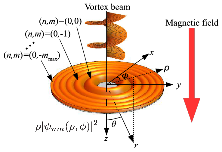
The quantized energy levels of 2DEG in the magnetic field $B$ are given by [37] $E_{N}=\hbar\omega_{c}\left(N+1/2\right)$, which usually appear by solving the Schrödinger equation in the Landau’s gauge, where $N=0,1,2,\dots$ is the Landau level index, and $\omega_{c}=eB/m_{e}$ is the cyclotron frequency with the elementary charge $e\left(>0\right)$, and the bare electron mass $m_{e}$. We here note that the electron mass $m_{e}$ should be interpreted as an effective mass $m_{e}^{\ast}=0.067m_{e}$ for GaAs. However, when we consider 2DEG interacting with the Bessel OV light beam, the symmetric gauge in the cylindrical coordinates becomes a natural choice. Hence, we consider 2DEG on with a circularly shaped disk geometry and take the cylindrical coordinates as shown in Fig.2.

The non-perturbative Hamiltonian for 2DEG under the magnetic field is given by

$$H_{0}=\frac{1}{2m_{e}}\left[-i\hbar\mathbf{\nabla}+e\mathbf{A}^{\text{ext}}(\mathbf{r})\right]^{2}$$

(18)

where $\mathbf{A}^{\text{ext}}(\mathbf{r})=\left(-By/2,Bx/2,0\right)$, and the magnetic field is along the $z$-axis direction. The energy spectrum is obtained by solving the Schrödinger equation $H_{0}\Psi=E\Psi$ which gives[38]

	$\displaystyle E_{n,m}$	$\displaystyle=\hbar\omega_{c}\left(n+\frac{|m|+m}{2}+\frac{1}{2}\right),$
	$\displaystyle n$	$\displaystyle=0,1,2,...,\text{and }m=0,\pm 1,\pm 2,...,$		(19)

where $m$ is the magnetic quantum number related to the angular momentum of the electron. The eigenfunction is also obtained as

	$\displaystyle\Psi_{nm}\left(\rho,\varphi,z\right)$	$\displaystyle=N_{nm}\mathrm{e}^{-\frac{\rho^{2}}{4l_{B}^{2}}}\left(\frac{\rho}{l_{B}}\right)^{|m|}L_{n}^{|m|}\left(\frac{\rho^{2}}{2l_{B}^{2}}\right)\frac{\mathrm{e}^{im\varphi}}{\sqrt{2\pi}}$
		$\displaystyle=R_{nm}\left(\rho\right)\frac{\mathrm{e}^{im\varphi}}{\sqrt{2\pi}},$		(20)

where $l_{B}=\sqrt{\hbar/eB}$ is the magnetic length, $N_{nm}=\left(n!/(n+|m|)!\right)^{1/2}2^{-|m|/2}l_{B}^{-1}$ is the normalization constant, and $L_{n}^{|m|}(x)$ is the associated Laguerre polynomials. In this picture, we call $n$ the principal quantum number. Its relation to ordinary Landau index $N$ is $N=n+(\left|m\right|+m)/2$. This leads to $N=n$ for states with $m\leq 0$. Each Landau level with given $N$ is multiply degenerated with respect to $n$ and $m$ due the finite system size with the degeneracy factor given by $S/(2\pi l_{B}^{2})$, where $S$ is the area of 2DEG.

For example, the lowest Landau level (LLL) $N=0$ is obtained by the condition $n+(\left|m\right|+m)/2=0$, which leads to $n=0$ and $m\leq 0$. The probability density for the electron with the wave function (3) has the maximal value at $\rho=\sqrt{2\left|m\right|+1}l_{B}$. This means that the electron is distributed on the circle with the radius $\sqrt{2\left|m\right|+1}l_{B}$. Because the expectation value of $r^{2}$ is given by $2(\left|m\right|+1)l_{B}^{2}$, we find that the electron state covers the area $2\pi l_{B}^{2}$. Then, the maximum $m$ for the disk geometry is given by[39]

$$m_{\text{max}}\simeq\frac{S}{2\pi l_{B}^{2}}=\frac{R^{2}}{2l_{B}^{2}},$$

(21)

which allows us to define the filling factor as

$$\nu\equiv\frac{N_{e}}{m_{\text{max}}}\simeq 2\pi l_{B}^{2}\frac{N_{e}}{\pi R^{2}},$$

(22)

where $N_{e}$ is the total number of electrons on the disk. Throughout this paper, we concentrate on the system with the filling factor $\nu=1$, where the Fermi energy lies in the gap between the LLL and the second Landau level (2LL). We display the energy diagram of the axial symmetric 2DEG system as shown in Fig.3.

Here, we investigate the interaction of a Landau-quantized 2DEG with the Bessel OV by applying the linear response theory. We start with the following total Hamiltonian, which contains the non-perturbative Hamiltonian (18) interacting with the vector potential of the OV:

$$H\mathbf{=}H_{0}+\Delta H=\frac{1}{2m_{e}}\left[-i\hbar\mathbf{\nabla}+e\mathbf{A}^{\text{ext}}(\mathbf{r})\right]^{2}-\bm{A}_{\ell,\sigma}^{\text{OV}}\cdot\mathbf{j},$$

(23)

where $\bm{A}_{\ell,\sigma}^{\text{OV}}$ is given by Eq. (16), and the electric current is determined by $\mathbf{j}=\frac{e}{m_{e}}\left(\mathbf{p}+e\mathbf{A}^{\text{ext}}\right)$. We neglect the electron spin.

The Kubo formula for $i$-component of the induced current is written as [40, 41]

	$\displaystyle\delta j_{i}\left(\omega\right)$	$\displaystyle=-\sum_{n,m}\sum_{n^{\prime},m^{\prime}}\left(f(E_{n,m})-f(E_{n^{\prime},m^{\prime}})\right)$
		$\displaystyle\times\frac{\langle n,m|j_{i}|n^{\prime},m^{\prime}\rangle\langle n^{\prime},m^{\prime}|\bm{A}_{\ell,\sigma}^{\text{OV}}\cdot\mathbf{j}|n,m\rangle}{E_{n,m}-E_{n^{\prime},m^{\prime}}+\hbar\omega+i\delta}.$		(24)

where $f(E_{n,m})$ is the Fermi distribution $f(\epsilon)=\left[\exp\beta\left(\epsilon-\mu\right)+1\right]^{-1}$ with a chemical potential $\mu$ and an inverse temperature $\beta$, and $|n,m\rangle$ is the electron wavefunction in Eq.(3). From now on, we assume zero-temperature limit and keeping the chemical potential lie between th LLL ($N=0$) and the second LL ($N=1$).

It should be mentioned that, although we work in the cylindrical coordinates, which manifest the symmetry of the OV, our final results, of course, are not specific to a particular coordinate system. Alternatively, we can consider the spherical coordinates and examine the multipole expansion by the vector spherical harmonics (VSH) of currents in Eq. (24) as discussed in Appendix B where we obtain the general expression in Eq. (69). We also show that the selection rules for the dipole transitions in Eq. (78) are consistent with the results obtained without multipole expansion in Eq. (31).

Let us now return to discussion without multipole expansion. To investigate the OV-induced photocurrent, we adopt the chiral basis $j_{\pm}(=j_{x}\pm ij_{y})$. First, we consider the matrix element of photocurrent $j_{\pm}$ that can be written as

$$\langle n,m|j_{\pm}|n^{\prime},m^{\prime}\rangle=i\frac{e}{\hbar}d(E_{n,m}-E_{n^{\prime},m^{\prime}})C_{n,m}^{n^{\prime},m^{\prime}}\delta_{m^{\prime},m\pm 1}$$

(25)

where $d(\ll R)$ is the thickness of 2DEG and we denote the radial integral as

$$C_{n,m}^{n^{\prime},m^{\prime}}=\int d\rho\rho^{2}R_{n^{\prime},m^{\prime}}(\rho)R_{n,m}(\rho).$$

(26)

Here, we obtain the selection rule $m^{\prime}=m\pm 1$ from the azimuthal integral $\int_{0}^{2\pi}\frac{d\varphi}{2\pi}\mathrm{e}^{i(m^{\prime}-m\pm 1)\varphi}$. After calculating the radial integral $C_{n,m}^{n^{\prime},m^{\prime}}$ and the energy factor $E_{n,m}-E_{n^{\prime},m^{\prime}}$ by Eq.(19), we can obtain the matrix elements of the photocurrent as

	$\displaystyle\langle n,m|j_{+}|n^{\prime},m+1\rangle$	$\displaystyle=\begin{cases}0\text{ \ \ \ \ \ \ \ \ \ \ \ \ \ \ for\hskip 3.0pt}n^{\prime}=n\text{,\hskip 3.0pt}m<0,\\ -iedl_{B}\omega_{c}\sqrt{2n+\left|m\right|+m+2}\\ \text{ \ \ \ \ \ \ \ \ \ \ \ \ \ \ \ \ \ for\hskip 3.0pt}n^{\prime}=n\text{, }m\geq 0,\\ 0\text{ \ \ \ \ \ \ \ \ \ \ \ \ \ \ \ for\hskip 3.0pt}n^{\prime}=n-1\text{,\hskip 3.0pt}m\geq 0,\\ iedl_{B}\omega_{c}\sqrt{2n+\left|m\right|+m+2}\\ \text{ \ \ \ \ \ \ \ \ \ \ \ \ \ \ \ \ \ for\hskip 3.0pt}n^{\prime}=n+1\text{,\hskip 3.0pt}m<0,\\ 0\text{ \ \ \ \ \ \ \ \ \ \ \ \ \ \ \ for otherwise,}\end{cases},$		(27)
	$\displaystyle\langle n,m|j_{-}|n^{\prime},m-1\rangle$	$\displaystyle=\begin{cases}0\text{ \ \ \ \ \ \ \ \ \ \ \ \ \ \ \ for\hskip 3.0pt}n^{\prime}=n\text{,\hskip 3.0pt}m\leq 0,\\ iedl_{B}\omega_{c}\sqrt{2n+\left|m\right|+m}\\ \text{ \ \ \ \ \ \ \ \ \ \ \ \ \ \ \ \ \ for\hskip 3.0pt}n^{\prime}=n\text{,\hskip 3.0pt}m>0,\\ -iedl_{B}\omega_{c}\sqrt{2n+\left|m\right|+m}\\ \text{ \ \ \ \ \ \ \ \ \ \ \ \ \ \ \ \ \ for\hskip 3.0pt}n^{\prime}=n-1\text{,\hskip 3.0pt}m\leq 0,\\ 0\text{ \ \ \ \ \ \ \ \ \ \ \ \ \ \ \ for\hskip 3.0pt}n^{\prime}=n+1\text{,\hskip 3.0pt}m>0,\\ 0\text{ \ \ \ \ \ \ \ \ \ \ \ \ \ \ \ for otherwise,}\end{cases}.$		(28)

For the filling factor $\nu=1$ $(n=0,m\leq 0)$, these matrix elements reduce to

	$\displaystyle\langle 0,m|j_{+}|n^{\prime},m+1\rangle$	$\displaystyle=\begin{cases}-iedl_{B}\omega_{c}\sqrt{2}\text{ \ \ \ \ \ \ \ for\hskip 3.0pt}n^{\prime}=0\text{,\hskip 3.0pt}m=0\\ iedl_{B}\omega_{c}\sqrt{2}\text{ \ \ \ \ \ for\hskip 3.0pt}n^{\prime}=1\text{,\hskip 3.0pt}m<0\\ 0\text{ \ \ \ \ \ \ \ \ \ \ \ \ \ \ \ \ \ \ \ \ \ \ for otherwise}\end{cases},$		(29)
	$\displaystyle\langle 0,m|j_{-}|n^{\prime},m-1\rangle$	$\displaystyle=0\text{ \ \ for all }n^{\prime},m.$		(30)

Therefore, we find that the transition is allowed only $N\rightarrow N+1$[41]. We summarize possible transitions from the LLL ($N=0$) to the second LL ($N=1$) as follows,

$$\left\{\begin{array}[c]{cccc}\left(n,m,N\right)&&\left(n^{\prime},m^{\prime},N^{\prime}\right)&\\ (0,0,0)&\rightarrow&(0,1,1)&\text{for }m=0\\ (0,m,0)&\rightarrow&(1,m+1,1)&\text{for }m<0\end{array}\right..$$

(31)

Next, we consider the matrix element of the minimal coupling of 2DEG with OV. As shown in Appendix A, the dipole approximation is justified in our model. Then the matrix element for the photon absorption in this approximation is obtained as

	$\displaystyle\langle n^{\prime},m^{\prime}|\bm{A}_{\ell,\sigma}^{\text{OV}}\cdot\mathbf{j}|n,m\rangle$	$\displaystyle\sim i\frac{e}{\hbar}(E_{n^{\prime},m^{\prime}}-E_{n,m})\langle n^{\prime},m^{\prime}|\bm{A}_{\ell,\sigma}^{\text{OV}}\cdot\mathbf{r}|n,m\rangle$
		$\displaystyle=A_{0}\frac{ed}{\hbar}\sqrt{\frac{k_{\perp}}{4\pi}}(E_{n,m}-E_{n^{\prime},m^{\prime}})D_{n,m,\ell}^{n^{\prime},m^{\prime}}$
		$\displaystyle\times\delta_{m^{\prime},m+\ell+\sigma},$		(32)

where we denoted the radial integral as

$$D_{n,m,\ell}^{n^{\prime},m^{\prime}}=\int d\rho\rho^{2}R_{n^{\prime},m^{\prime}}(\rho)R_{n,m}(\rho)J_{\ell}(k_{\perp}\rho).$$

(33)

We also obtain the selection rule $m^{\prime}=m+\ell+\sigma$ from the azimuthal integral $\int_{0}^{2\pi}\frac{d\varphi}{2\pi}\mathrm{e}^{i(m-m^{\prime}+\ell+\sigma)\varphi}$, where $\sigma=\pm 1$. This means that the OV can transfer its TAM to the electron via the dipole interaction.

We note that, when we fix the filling factor $\nu=1$ (the chemical potential lies between $N=0$ and $N=1$), the left-handed current is not induced. Therefore, only the right-handed current arises by transferring the optical TAM, $J=1$. Because the OV carries the SAM $\sigma=\pm 1$, the OAM and SAM must be $\ell=0$, $\sigma=1$, or $\ell=2$, $\sigma=-1$, respectively, with the other transitions being prohibited.

On the other hand, if we apply the external magnetic field anti-parallel to the light traveling, since it corresponds to the time inverse, the electron in the LLL carries positive value angular momentum. Then, to excite the electron in the LLL, the electron can absorb the optical TAM $J=-1$. As a result, the possible absorptions are reduced to $\ell=0$, $\sigma=-1$, and $\ell=-2$, $\sigma=1$.

Next, we calculate the photocurrent using the Kubo formula. For the transition from $N=0$ to $N=1$ with $\nu=1$, the OV-induced current (24) reduces to

$$\delta j_{\ell}^{+}\left(\omega,B\right)=-i\frac{F^{\ell}\left(B\right)}{\hbar\omega-\hbar\omega_{c}+i\delta},$$

(34)

where $\ell=0$ or $2$ and the factors $F^{\ell}$ are given by

$$F^{\ell}\left(B\right)=A_{1}C_{0,0}^{0,1}D_{0,0,\ell}^{0,1}+A_{1}\sum_{m<0}^{-m_{\max}}C_{0,m}^{1,m+1}D_{0,m,\ell}^{1,m+1},$$

(35)

with $A_{1}=A_{0}e^{2}d^{2}\omega_{c}^{2}\sqrt{k_{\perp}/4\pi}/V$. In the summation with respect to $m$, by using the explicit form, $L_{1}^{k}\left(x\right)=1+k-x$, only one term corresponding to an edge current along the circle with the radius $R$ survives. The other terms corresponding to the bulk currents cancel each other. After some algebra, we obtain

	$\displaystyle F^{\ell}\left(B\right)$	$\displaystyle\sim\frac{F_{0}}{\sqrt{\alpha^{5}}}\left(\frac{1+\alpha^{2}}{\alpha^{2}}\frac{\Phi_{0}^{2}}{\lambda_{e}^{2}R^{2}B^{2}}\left[1+\frac{\Phi_{0}}{2\pi R^{2}B}\right]\mathrm{e}\right)^{\frac{\pi R^{2}}{\Phi_{0}}B}$
		$\displaystyle\times\int_{0}^{k_{\perp}R}dxx^{2m_{\text{max}}\left(B\right)+3}\mathrm{e}^{-\frac{x^{2}}{2k_{\perp}^{2}l_{B}^{2}}}J_{\ell}(x),$		(36)

where $\ell$ is $0$ or $2$, $F_{0}=A_{0}e^{2}d^{2}c^{2}/V\sqrt{2\pi\lambda_{e}\mathrm{e}}$, $x=k_{\perp}\rho$, which has an order of magnitude of unity. $\Phi_{0}=2\pi\hbar/e$ is the flux quantum, and $\lambda_{e}=2\pi\hbar/m_{e}c$ is the electron Compton wavelength.

In this section, we present a physical interpretation on the reason why the bulk currents are cancelled out, based on the coherent state representation. Introducing the Larmor radius vector $\bm{\eta}$ and the guiding center vector $\bm{r}_{0}=\left(x_{0},y_{0}\right)\$satisfying$\ \left(\eta_{x},\eta_{y}\right)=\left(x-x_{0},y-y_{0}\right)$, we can rewrite the 2DEG Hamiltonian as

$$H_{0}=\frac{1}{2}m_{e}\omega_{c}^{2}\left(\eta_{x}^{2}+\eta_{y}^{2}\right)=\frac{1}{2}m_{e}v_{\perp}^{2},$$

(37)

where we note the relation $\left|\bm{\eta}\right|=v_{\perp}/\omega_{c}$. We can then define the non-commuting operators which satisfy

$$\left[\hat{\eta}_{x},\hat{\eta}_{y}\right]=-il_{B},\ \left[\hat{x}_{0},\hat{y}_{0}\right]=il_{B}.$$

(38)

We find that one electron occupies the area determined by the uncertainty principle:

$$\Delta S=\Delta x_{0}\Delta y_{0}=2\pi l_{B}^{2}.$$

(39)

Then we can define the ladder operators

	$\displaystyle a$	$\displaystyle=\frac{1}{\sqrt{2}l_{B}}\left(\hat{\eta}_{x}-i\hat{\eta}_{y}\right),\ a^{{\dagger}}=\frac{1}{\sqrt{2}l_{B}}\left(\hat{\eta}_{x}+i\hat{\eta}_{y}\right),$
	$\displaystyle b$	$\displaystyle=\frac{1}{\sqrt{2}l_{B}}\left(\hat{x}_{0}+i\hat{y}_{0}\right),\ b^{{\dagger}}=\frac{1}{\sqrt{2}l_{B}}\left(\hat{x}_{0}-i\hat{y}_{0}\right),$		(40)

with $\left[a,a^{{\dagger}}\right]=\left[b,b^{{\dagger}}\right]=1$, and $\left[a,b^{({\dagger})}\right]=0$. The eigenstates are thus determined by the two integer quantum numbers, $N$ and $M$, associated with the two ladder operators,

	$\displaystyle a^{{\dagger}}|N,M\rangle$	$\displaystyle=\sqrt{N+1}|N+1,M\rangle,\text{ \ }a|N,M\rangle=\sqrt{N}|N-1,M\rangle$
		$\displaystyle\text{\ \ \ \ \ \ \ \ \ \ \ \ \ \ \ for }N>0;$		(41)
	$\displaystyle b^{{\dagger}}|N,M\rangle$	$\displaystyle=\sqrt{M+1}|N,M+1\rangle,\text{ \ }b|N,M\rangle=\sqrt{M}|N,M-1\rangle$
		$\displaystyle\text{\ \ \ \ \ \ \ \ \ \ \ \ \ \ \ for }M>0.$		(42)

Then in terms of the two ladder operators, the Hamiltonian and the angular momentum operator are written by

$$H_{0}=\hbar\omega_{c}\left(a^{{\dagger}}a+\frac{1}{2}\right)=\hbar\omega_{c}\left(N+\frac{1}{2}\right)$$

(43)

$$L_{z}=\hbar\left(a^{{\dagger}}a-b^{{\dagger}}b\right)=\hbar\left(N-M\right).$$

(44)

Here, comparing above eigenvalues with Eq.(19) and $L_{z}=\hbar m$, we can determine the relation between $n$, $m$ and $N$, $M$ as

$$N=n+\frac{\left|m\right|+m}{2},\ M=n+\frac{\left|m\right|-m}{2}.$$

(45)

The average value of the guiding center operator $\bm{\hat{r}}_{0}$ gives

$$\left\langle N,M\left|\bm{\hat{r}}_{0}\right|N,M\right\rangle=0,$$

(46)

but its absolute value leads to

$$\left\langle\left|\bm{r}_{0}\right|\right\rangle_{N,M}\equiv\sqrt{\left\langle N,M\left|\bm{\hat{r}}_{0}^{2}\right|N,M\right\rangle}=l_{B}\sqrt{2M+1}.$$

(47)

Similarly, the average value of Larmor radius operator gives

$$\left\langle N,M\left|\bm{\hat{\eta}}\right|N,M\right\rangle=0,$$

(48)

but its absolute value is given by

$$\left\langle\left|\bm{\eta}\right|\right\rangle_{N,M}\equiv\sqrt{\left\langle N,M\left|\bm{\hat{\eta}}^{2}\right|N,M\right\rangle}=l_{B}\sqrt{2N+1}.$$

(49)

Therefore, the arbitrary state $|N,M\rangle$ distributes at the center of the Larmor motion with radius $\left\langle\left|\bm{\eta}\right|\right\rangle_{N,M}=l_{B}\sqrt{2N+1}$ is located at the position of guiding center

$$\left\langle\left|\bm{r}_{0}\right|\right\rangle_{N,M}=l_{B}\sqrt{2M+1}.$$

(50)

The geometric meaning of this is illustrated in Fig. 4. When we focus on the LLL, that is, $n=0$ and$\ m\leq 0$, we see $N=0$ and $M=\left|m\right|$. Therefore, the guiding center in the LLL is $\left\langle\left|\bm{r}_{0}\right|\right\rangle_{0,\left|m\right|}=l_{B}\sqrt{2\left|m\right|+1}$, and the Larmor radius in it is $\left\langle\left|\bm{\eta}\right|\right\rangle_{0,\left|m\right|}=l_{B}$.

This kind of distribution can semi-classically be described by the coherent states. We now introduce the displacement operators

$$D\left(x_{0},y_{0}\right)=e^{-i\left(x_{0}\hat{y}_{0}-y_{0}\hat{x}_{0}\right)/l_{B}^{2}},\ D\left(\eta_{x},\eta_{y}\right)=e^{i\left(\eta_{x}\hat{\eta}_{y}-\eta_{y}\hat{\eta}_{x}\right)/l_{B}^{2}}.$$

(51)

The first displacement operator $D\left(x_{0},y_{0}\right)$ generates a displacement to the position at the guiding center $\left|\bm{r}_{0}\right|=\sqrt{x_{0}^{2}+y_{0}^{2}}$. Since $D\left(x_{0},y_{0}\right)$ commutes with the Hamiltonian $H_{0}$, the guiding center is the constant of motion. Therefore, the Hamiltonian $H_{0}$ does not depend on quantum number $M$. On the other hand, the second displacement operator $D\left(\eta_{x},\eta_{y}\right)$ generates a displacement to the position $\left|\bm{\eta}\right|=\sqrt{\eta_{x}^{2}+\eta_{y}^{2}}$. Since $D\left(\eta_{x},\eta_{y}\right)$ does not commute with the Hamiltonian $H_{0}$, the coherent state is not an eigenstate of the Hamiltonian.

Applying these displacement operators to the ground state $|0,0\rangle=|n_{a}=0,n_{b}=0\rangle$, we can thus construct the coherent state,

	$\displaystyle|X_{0},Y_{0};\eta_{x},\eta_{y}\rangle$	$\displaystyle=D\left(\eta_{x},\eta_{y}\right)D\left(x_{0},y_{0}\right)|0,0\rangle$
		$\displaystyle=e^{-\left(\left|\alpha\right|^{2}+\left|\beta\right|^{2}\right)/2}e^{\alpha a^{{\dagger}}}e^{\beta b^{{\dagger}}}|0,0\rangle,$		(52)

where $\alpha$ and $\beta$ are eigenvalues of the annihilation operators $a$ and $b$ of the eigenstate $|x_{0},y_{0};\eta_{x},\eta_{y}\rangle$. That is, these eigenstates satisfy

	$\displaystyle a|x_{0},y_{0};\eta_{x},\eta_{y}\rangle$	$\displaystyle=\frac{\eta_{x}-i\eta_{y}}{\sqrt{2}l_{B}}|x_{0},y_{0};\eta_{x},\eta_{y}\rangle$
		$\displaystyle=\frac{\left|\bm{\eta}\right|e^{-i\varphi}}{\sqrt{2}l_{B}}|x_{0},y_{0};\eta_{x},\eta_{y}\rangle,$		(53)
	$\displaystyle b|x_{0},y_{0};\eta_{x},\eta_{x}\rangle$	$\displaystyle=\frac{x_{0}+iy_{0}}{\sqrt{2}l_{B}}|x_{0},y_{0};\eta_{x},\eta_{y}\rangle$
		$\displaystyle=\frac{\left|\bm{r}_{0}\right|e^{i\varphi}}{\sqrt{2}l_{B}}|x_{0},y_{0};\eta_{x},\eta_{y}\rangle,$		(54)

and the eigenvalues $\alpha$ and $\beta$ are given by

	$\displaystyle\alpha$	$\displaystyle=\frac{\eta_{x}-i\eta_{y}}{\sqrt{2}l_{B}}=\frac{\left|\bm{\eta}\right|e^{-i\varphi}}{\sqrt{2}l_{B}},$		(55)
	$\displaystyle\beta$	$\displaystyle=\frac{x_{0}+iy_{0}}{\sqrt{2}l_{B}}=\frac{\left|\bm{r}_{0}\right|e^{i\varphi}}{\sqrt{2}l_{B}}.$		(56)

To see the absence of bulk currents, we pay our attention to one coherent state at the guiding center $\bm{r}_{0}$, which produces the circular current by the Larmor motion with radius $\left|\bm{\eta}\right|$. Because of the uncertainty (39), it seems that the circular current flows the edge of the area $\Delta S$. When the LLs state can be constructed by the superposition of the coherent states, the superposition produces contact points of the circular current at the center $\bm{r}_{0}$ with the surrounding circular currents. Thus, the circular current at the center $\bm{r}_{0}$ is canceled by the surrounding circular current. Such the cancellation occurs on whole system except to the edge, we can say the bulk currents are all cancelled out, i.e.,

$$\bm{j}_{\text{bulk}}=0.$$

(57)

References

• [1] J. H. Poynting, Proc. R. Soc. Lond. Ser. A82, 560 (1909).
• [2] R. A. Beth, Phys. Rev. 48, 471 (1935).
• [3] R. A. Beth, Phys. Rev. 50, 115 (1936).
• [4] L. Allen, M. W. Beijersbergen, R. J. C. Spreeuw, and J. P. Woerdman, Phys. Rev. A 45, 8185 (1992).
• [5] A. Mair, A. Vaziri,G. Weihs, and A. Zeilinger, Nature 412, 313 (2001).
• [6] J. Durnin, J. Opt. Soc. Am. B 4, 651 (1987).
• [7] D. L. Andrews, Structured Light and Its Applications: An Introduction to Phase-Structured Beams and Nanoscale Optical Forces (Academic Press, Amsterdam, 2008) .
• [8] Sonja Franke-Arnold, Philosl. Trans. R. Soc. A 375, 20150435 (2017).
• [9] S. M. Barnett, M. Babiker, and M. J. Padgett, Philos. Trans. R. Soc. A 375, 20150444 (2017).
• [10] J. Durnin, J.J. Miceli and J.H. Eberly, Phys. Rev. Lett. 58, 1499 (1987).
• [11] G. Indebetouw, J. Opt. Soc. Am. A 6, 150 (1989).
• [12] A. Vasara, J. Turunen and A.T. Friberg, J. Opt. Soc. Am. A 6, 1748 (1989).
• [13] A.J. Cox and D.C. Dibble, J. Opt. Soc. Am. A 9, 282 (1992).
• [14] B. Amos, and P. Gill, Meas. Sci. Technol., 6, 248 (1995).
• [15] H. He, M. E.J. Friese, N. R. Heckenberg, and H. Rubinsztein-Dunlop, Phys. Rev. Lett. 75, 826 (1995).
• [16] M. E. J. Friese, T. A. Nieminen, N. R. Heckenberg, and H. Rubinsztein-Dunlop, Nature 394, 348 (1998).
• [17] J. Hamazaki, R. Morita, K. Chujo, Y. Kobayashi, S. Tanda, and T. Omatsu, Opt. Express 18, 2144 (2010).
• [18] M. F. Andersen, C. Ryu, P. Cladé, V. Natarajan, A. Vaziri, K. Helmerson, and W. D. Phillips, Phys. Rev. Lett. 97, 170406 (2006).
• [19] G. F. Quinteiro and P. I. Tamborenea, EPL 85, 47001 (2009).
• [20] J. Wätzel, A. S. Moskalenko, and J. Berakdar, Opt. Express 20, 27792 (2012).
• [21] M. B. Farīas, G. F. Quinteiro, and P. I. Tamborenea, Eur. Phys. J. B 86, 432 (2013).
• [22] K. Sakai, K. Nomura, T. Yamamoto, and K. Sasaki, Sci. Rep. 5, 8431 (2015).
• [23] K. Shintani, K. Taguchi, Y. Tanaka, and Y. Kawaguchi, Phys. Rev. B 93, 195415 (2016).
• [24] H. Fujita and M. Sato, Phys. Rev. B 95, 054421 (2017).
• [25] C. T. Schmiegelow, J. Schulz, H. Kaufmann, T. Ruster, U. G. Poschinger, and F. Schmidt-Kaler, Nat. Commun. 7, 12998 (2016).
• [26] A. Afanasev, C. E. Carlson, C. T. Schmiegelow, J. Schulz, F. Schmidt-Kaler, and M. Solyanik, New J. Phys. 20, 023032 (2018).
• [27] M. Solyanik-Gorgone, A. Afanasev, C. E. Carlson, C. T. Schmiegelow, and F. Schmidt-Kaler, J. Opt. Soc Am. B 36, 565 (2019).
• [28] M. Babiker, C. R. Bennett, D. L. Andrews, and L.C. Dávila Romero, Phys. Rev. Lett. 89, 143601 (2002).
• [29] S. M. Lloyd, M. Babiker, and J. Yuan, Phys. Rev. A 86, 023816 (2012).
• [30] K. Shigematsu, K. Yamane, R. Morita, and Y. Toda, Phys. Rev. B 93, 045205 (2016).
• [31] W. Kohn, Phys. Rev. 123, 1242 (1961).
• [32] H. T. Takahashi, I. Proskurin, and J. Kishine, J. Phys. Soc. Jpn. 87, 113703 (2018).
• [33] T. Thonhauser, D. Ceresoli, D. Vanderbilt, and R. Resta, Phys. Rev. Lett. 95, 137205 (2005).
• [34] T. Yoda, T. Yokoyama, and S. Murakami, Nano Lett. 18, 916–920 (2018).
• [35] O. Matula, A. G. Hayrapetyan, V. G. Serbo, A. Surzhykov, and S. Fritzsche, J. Phys. B 46, 205002 (2013).
• [36] U. D. Jentschura and V. G. Serbo, Phys. Rev. Lett. 106, 013001 (2011).
• [37] L. D. Landau and E. M. Lifshitz, Quantum Mechanics: Non-Relativistic Theory, 3rd ed., (Pergamon, Oxford, 1977).
• [38] C. G. Darwin, Math. Proc. Cambridge Philos. Soc. 27, 86 (1931).
• [39] D. Yoshioka, The Quantum Hall Effect (Springer-Verlag Berlin Heidelberg, 2002)
• [40] R. Kubo, J. Phys. Soc. Jpn. 12, 570 (1957).
• [41] T. Ando, J. Phys. Soc. Jpn. 38, 989 (1975).
• [42] H. Fujita, Y. Tada, and M. Sato, arXiv:1811.10617.
• [43] R. G. Barrera, G. A. Estévez, and J. Giraldo, Eur. J. Phys. 6, 287 (1985).