Perturbations of the Lambda-CDM model in a dynamical systems perspective
Abstract
The observational success and simplicity of the CDM model, and the explicit analytic perturbations thereof, set the standard for any alternative cosmology. It therefore serves as a comparison ground and as a test case for methods which can be extended and applied to other cosmological models. In this paper we introduce dynamical systems and methods to describe linear scalar and tensor perturbations of the CDM model, which serve as pedagogical examples that show the global illustrative powers of dynamical systems in the context of cosmological perturbations. We also study the asymptotic properties of the shear and Weyl tensors and discuss the validity of the perturbations as approximations to the Einstein field equations. Furthermore, we give a new approximation for the linear growth rate, , where is the cosmological redshift, , while is the background scale factor, and show that it is much more accurate than the previous ones in the literature.
1 Introduction
This paper is the first in a series of papers dealing with cosmological perturbations by means of dynamical systems formulations and methods. We will show how a wide variety of increasingly complex problems can be formulated as dynamical systems and how powerful dynamical systems methods can be applied to yield insights about cosmological perturbations. In particular, this will make it possible to apply approximation techniques from the theory of dynamical systems and to obtain illustrative pictures as well as mathematically rigorous results about the global structure of the various models solution spaces, thereby also providing a context for especially physically interesting solutions. Our aim is thus to provide a useful complement to traditional approaches to cosmological perturbations. Step by step we will introduce increasingly sophisticated models and methods. In this paper we focus on first order scalar and tensor perturbations of the spatially flat CDM model with dust and a positive cosmological constant . Since this model is mathematically simple and is compatible with a wide range of observations it is a natural choice as a first example to illustrate the most simple aspects of our dynamical systems approach to perturbative cosmology. Moreover, due to their observational success they provide a comparative testing ground for any observational contender.
Dynamical systems have been used before to analyze cosmological linear scalar perturbations in general relativity (GR) with an open Robertson-Walker (RW) geometry as background, see [24] and references therein. These models turn out to be somewhat easier to handle than models with a spatially flat background,11 1 In contrast to the spatially flat RW models, is always bounded for the spatially open models if the energy density is non-negative. This is due to how the spatial curvature term appears in the background Gauss constraint, which also can be used to solve for . Since appears in connection with the spatial derivatives of the perturbed equations, this significantly simplifies the analysis of the perturbed field equations in the open case. which is what we will focus on. However, there has also been some previous work on dynamical systems in this area in GR, notably [4] which treated dust and radiation as a single fluid.
The main foundation for standard cosmology is the spatially flat RW geometry, characterized by a line element that can be written as
| (1) |
where is the background scale factor, is the flat spatial 3-metric, which in Cartesian coordinates is given by , and is the background Hubble variable. The different time coordinates above are the clock time , the conformal time , and the -fold time
| (2) |
where describes the number of background -foldings with respect to some reference epoch at which (a negative describes the number of -folds before the reference time). If this reference epoch is the present time, then
| (3) |
where is the cosmological background redshift. Much of the work in cosmological perturbation theory uses the clock time or the conformal time , but we find it more convenient to use the -fold time as the starting point for our work.
The outline of the paper is as follows. In the next section we describe some aspects of the framework of our new dynamical systems approach to cosmological perturbations. In Section 3 we consider linear scalar perturbations of the CDM models from a dynamical systems perspective. We also present and discuss previously known analytic results in the present context. In addition we describe and discuss various asymptotic approximation methods and give a new more accurate approximation for the so-called linear growth rate. In Section 4 we consider the linear tensor perturbations from a dynamical systems perspective. In Section 5 we relate the present work to the full state space of GR and discuss the validity of the perturbations as approximations to the Einstein field equations. This is done by comparing asymptotic perturbative results with asymptotic results in GR for the Hubble-normalized comoving shear and Weyl tensor. The paper is concluded with some final remarks in Section 6.
2 Dynamical systems approach to cosmological perturbations
Our aim is to analyze cosmological perturbations by formulating the governing equations as regular dynamical systems on compact state spaces. In this paper we will consider first order scalar and tensor perturbations of the spatially flat CDM models with dust and a positive cosmological constant . However, since similar methods apply to models whose matter content consists of a perfect fluid with a barotropic equation of state and with, or without, a cosmological constant it is useful to point out some common features these models exhibit. The governing equation for scalar perturbations for this class of models can be a single second order partial differential equation (e.g. the Bardeen equation) or a system of two coupled first order partial differential equations (e.g. the Kodama-Sasaki equations), depending on the choice of gauge and the choice of variables, see e.g. [21] and references therein. For an arbitrary equation of state these governing equations will contain the spatial Laplacian . This is also the case for the tensor perturbations which obey a linear second order differential master equation for a single variable.
In order to obtain ordinary differential equations (ODEs) we make a spatial Fourier decomposition of the perturbation variables, which involves replacing the perturbation variables by their Fourier coefficients and making the transition
| (4) |
where is the wave number. At this stage if we have a second order ODE as a governing equation we would replace it by a system of two coupled first order ODEs by using the first order time derivative as an independent variable. In this way the Einstein field equations for first order scalar and tensor perturbations of the models under consideration can be written as a system of linear ODEs of the form
| (5a) | ||||
| (5b) | ||||
for two linear perturbation variables and , where a ′ denotes differentiation with respect to the -fold time . Due to the spatial Fourier decomposition one obtains complex variables, but thanks to that the differential equations are linear, real and complex parts satisfy the same equations, and therefore we can without loss of generality consider and to be real, as are , whose specific form is determined by the background model. This is exemplified in detail in section 4 where tensor perturbations are treated.
The next step toward obtaining a regular dynamical system on a bounded state space is to introduce polar coordinates , , which thanks to the linearity of the equations lead to a decoupling of an equation for and a reduction of the system of two linear ODEs (5) to one nonlinear ODE for :
| (6) |
However, locally it is more convenient to replace with
| (7) |
which results in a Riccati ODE given by
| (8) |
which describes the essential “reduced” dynamics of the problem since, e.g., can be obtained as a quadrature from the decoupled equation once the equation for has been solved.
To obtain a dynamical system, i.e. a system of first order autonomous ODEs, that incorporates the dynamics described by the non-autonomous ODE (8) or (6), we introduce a new dependent variable , where is a non-negative, bounded and increasing function. It follows that satisfies an autonomous ODE of the form
| (9) |
Note that is obtained by differentiating and then expressing in terms using the inverse function . This equation is adjoined to (8) or (6), thereby yielding a 2-dimensional dynamical system for or .
In practice, however, we have found it convenient to use the relation to express as a function of rather than . In particular we write in terms of a subsidiary function according to
| (10) |
where is a non-negative, increasing, explicitly invertible, and suitably differentiable function which satisfies and when . This ensures that is a non-negative, bounded and increasing function that satisfies and . To find the function in (9), differentiate (10) with respect to using and then express in terms of using (10).
Augmenting the ODE (6) for with the ODE (9) for yields the dynamical system
| (11a) | ||||
| (11b) | ||||
where the functions are expressed as functions of . The state space for this system is a finite cylinder in which all orbits (i.e., solution trajectories), begin at the boundary and end at the boundary . We thus extend the state space to include these boundaries, which we refer to as the (extended) compactified state space cylinder . Note that can be regarded as a bounded time variable for which and correspond to and , respectively.
As mentioned, for local analysis it is more convenient to use instead of , which results in the system
| (12a) | ||||
| (12b) | ||||
In this representation traversing the infinite strip defined by and twice corresponds to making one revolution on the state space cylinder with the global coordinates and .22 2 The reason for traversing the strip twice is that , i.e., the mapping is two-to-one, although note that the right hand side of (6) has a periodicity .
The key to implementing the above procedure is to make an appropriate choice for the function that determines the new dependent variable through equation (10). In a particular application the choice is motivated by the form of the coefficient functions in the initial system (5). We will use this procedure in the following sections to describe the scalar and tensor perturbations of the CDM model.
3 Dynamical systems approach to scalar perturbations of CDM
Linear scalar perturbations of a spatially flat RW background geometry can be described by
| (13) |
where are the metric scalar perturbation variables (see e.g. Uggla and Wainwright (2018) [21].) The scalar matter perturbations for CDM are given by the first order fractional matter density perturbation
| (14) |
where the superscripts denote the order of the perturbation. The scalar velocity perturbation is defined by the first order perturbation of the spatial covariant 4-velocity components according to the relation
| (15) |
Setting fixes the spatial gauge and covers most of the familiar gauges, although it excludes the synchronous gauge (for a recent work using the synchronous gauge, see e.g. [8], and also [23] and [21] for further discussions and references). The temporal gauge can be fixed in a number of ways, e.g., by setting to zero one of the variables , , , . We use the following terminology and subscripts to label the gauges:
- i)
Poisson (Newtonian, longitudinal) gauge, subscript p, defined by ,
- ii)
uniform curvature gauge, subscript c, defined by ,
- iii)
total matter (comoving) gauge, subscript v, defined by .
As shown in e.g. [21] each choice leads to a different system of governing equations. In particular, for linear perturbations the uniform (flat) curvature gauge leads to a simple system of two first order partial differential equations, which form a natural starting point for a dynamical systems analysis. We obtain this system of equations from [21], where it is given in the following form:33 3 See equations (10), (54a) and (54b) in [21]. We have dropped superscripts (1) on the perturbation variables, and have set since we are considering a barotropic fluid.
| (16a) | ||||
| (16b) | ||||
with
| (17a) | |||
| Here is the background deceleration parameter, defined by either of the following forms, , where . The background Einstein equations relate to according to ([21], equation (4)): | |||
| (17b) | |||
For the CDM model we have44 4 See, for example, [21], Appendix B.
| (18) |
As basic perturbation variables for the CDM model we choose , where we have scaled with to obtain a dimensionless quantity, as discussed in [21] and [23]. We now specialize the governing equations (16) to the CDM model, using equations (17) and (18). After expanding the derivatives and replacing by ′ we obtain
| (19a) | ||||
| (19b) | ||||
Since the Laplacian has dropped out, there is no need for a spatial Fourier decomposition. The system (19), which is of the form (5), constitutes the starting point for transforming the governing equations into a dynamical system.
We now digress to describe the background dynamics of the CDM model in order to obtain the -dependence of . The density parameters are given by
| (20) |
which implies that
| (21) |
Since it follows from (21) that
| (22) |
3.1 Derivation of the dynamical systems
The metric perturbations in the uniform curvature gauge
We have shown that perturbations of the CDM model are described by the system of ODEs (19) which we repeat here:
| (23a) | ||||
| (23b) | ||||
with variables . This problem is explicitly solvable, and we will later give the solution. Here, however, we will use it as a first illustration of our dynamical systems approach. We therefore introduce , as in (7), but give a subscript, , as a reminder that we are using the uniform curvature gauge, thus
| (24) |
It follows from (23) that
| (25) |
To complete the process of constructing a dynamical system we now have to make a choice for the additional independent variable . It follows from equation (22) that
| (26) |
which suggests that we choose55 5 The second expression is useful for the calculation that follows.
| (27) |
In other words the function in (10) is given by , which has the desired properties. Differentiating (27) with respect to yields
| (28) |
after expressing in terms of using (27) again. This is the desired autonomous ODE for . Note that and that is an increasing function, as required. We finally use that in equation (25). The resulting equation, with (28), comprises the desired (analytic) dynamical system as follows:
| (29a) | ||||
| (29b) | ||||
Since is defined by the ratio of two metric coefficients, one orbit of the above system corresponds to a one-parameter family of solutions. Furthermore, the solutions for the dynamical system (29) correspond to solutions with all possible (non-zero) values of since is incorporated in the definition of . In order to solve for one has to impose an initial condition at , which corresponds to the initial epoch , of the form where is an arbitrary spatial function. Note that the initial value of , where was chosen in order to arrive at a simple form for (29) and is given by (27), is where is the initial value of .
Finally we note that the full dynamical system in the uniform curvature gauge consists of the state space vector governed by the equations (23) and (29b). This state space can then be covered by using polar coordinates , which leads to a decoupling of from a dynamical system with a reduced state space vector . Locally it is, however, more convenient to use and as the decoupled variable, which obeys
| (30) |
This equation is easily solved as a quadrature once a solution has been obtained, thereby also yielding the second constant of the motion which together with the constant of the motion for the reduced system for characterizes the various scalar perturbations.
The fractional density perturbation in the total matter gauge
The density contrast is defined by
| (31) |
where is the background matter density and is the linear density perturbation. The comoving density contrast , the gauge invariant that equals in the the total matter/comoving gauge, plays a central role in observational cosmology. Since satisfies a second order evolution equation we can apply our method to analyze its behaviour from a dynamical systems perspective. In the CDM universe this evolution equation has the following form when using -fold time :66 6 This evolution equation has been given in a general context in Uggla and Wainwright (2018) [21], equation (71a.b). When specialized to CDM and to first order perturbations, equation (71a) reads , where the differential operator in (71b) reduces to Since we obtain our equation (31). To avoid confusion we note that the usual density contrast is defined by normalizing with , while in [21] is defined by normalizing with . In the CDM universe these two normalizations are the same (see [21], Appendix B).
| (32) |
In order to formulate this differential equation as a dynamical system we use as basic variables, and define
| (33) |
in accordance with equation (7).
We obtain the ODE for by differentiating (33) using (32), and we make the same choice (27) of as before. This results in the following dynamical system
| (34a) | ||||
| (34b) | ||||
This formulation of the evolution equations which is based on differs from the system that is based on . However, and are closely related, as will be shown later.
3.2 Dynamical systems analysis
In this section we use dynamical systems methods to obtain qualitative information about the family of all solutions of the perturbed field equations, including asymptotic descriptions of the solutions at early and late times.
The uniform curvature gauge
When using the uniform curvature gauge the differential equations that define the reduced dynamical system are given by equations (29), which we here repeat for the reader’s convenience:
| (35a) | ||||
| (35b) | ||||
The associated state space is the infinite strip:
| (36) |
with boundaries and . Alternatively we can use the angular variable defined by , which yields the reduced regular global state space which is a finite section of a cylinder , as discussed in section 2.
The analysis of this dynamical system is straightforward. Equation (35b) shows that all the fixed points of the system lie on the boundaries and , and that each orbit is past asymptotic to a fixed point on and future asymptotic to a fixed point on . The local stability of the fixed points can be determined in the usual way by linearizing the differential equations.
When specialized to the and boundaries the differential equation (35a) results in the following equations:
| (37a) | ||||
| (37b) | ||||
It follows that on the boundary there are two fixed points (four in the case of , although they are connected by the discrete symmetry and thereby given by the two fixed points for ):77 7 The first subscript on a fixed point denotes the value of while the + (-) denotes the larger (smaller) value of .
| (38a) | ||||||
| (38b) | ||||||
Linearization shows that the fixed point is a hyperbolic saddle and that a single orbit originates from . To obtain an analytical approximation for this special orbit, we make a series expansion for in powers of and use the system (29) to solve for the coefficients,88 8 This can be mathematically justified be relating this series expansion to a so-called Picard expansion, see e.g. [17] and references therein. which leads to
| (39) |
for and close to zero. Next, linearization shows that the fixed point is a hyperbolic source, and hence a one-parameter family of orbits originates from . A series expansion in results in
| (40) |
where is a spatial function that parameterizes the orbits, depending on the spatial position.
Inserting the series expansion (40) into equation (30) for shows that toward the past for all orbits that originate from (to leading order it suffices to insert into (30)). In contrast inserting (39) into (30) shows that is finite asymptotically for the orbit that originates from . Since (see equation (61) below), it follows that the orbit that originates from is the only orbit along which the perturbations remain finite into the past i.e. as . Below we will identify this orbit with the so-called growing mode solution toward the future. Along all other orbits into the past, i.e., solutions that originate from , (some of) the perturbations increase without bound and hence will not asymptotically approximate solutions of the full Einstein equations. This is related to the fact that a general solution of the perturbed Einstein equations for scalar CDM perturbations is a linear combination of a so-called growing mode and a decaying mode, where the latter has the property that it becomes unbounded into the past.
On the boundary it follows from (37b) that the fixed points are given by
| (41a) | ||||||
| (41b) | ||||||
Linearization shows that the fixed point is a hyperbolic saddle that attracts a single orbit that is past asymptotic to . A series expansion in yields:
| (42) |
Finally, linearization shows that the fixed point is a hyperbolic sink, which implies that a one-parameter family of orbits is asymptotic to . A series expansion in results in
| (43) |
where is a spatial function that parameterizes the orbits, depending on the spatial position.
The preceding analysis of the stability of the fixed points enables one to predict the qualitative form of the state space (36) in figure 1 which shows the fixed points, the special heteroclinic orbits (i.e. solution trajectories that originate and end at two distinct fixed points), , (note that equation (35a) shows that this latter orbit is the invariant set , which in turn corresponds to the invariant set of equation (23a)), and , together with some typical orbits of the dynamical system (35). The most significant aspect of the state space in figure 1 is the heteroclinic orbit , the growing mode solution, which represents the most physically important solution of the perturbation equations (actually a one parameter family of solutions), and which thereby is the primary focus in cosmological perturbation theory. Note also that due to its observational success, any observational contender must presumably result in a solution trajectory in and that is quite similar to that of the growing mode solution for the observational redshift range.


As a final side remark we note the following about the heteroclinic growing mode orbit . Since is a saddle point and is a local sink, this orbit acts as an “attractor solution” toward the future of nearby orbits, reminiscent of “attractor solutions” in inflationary cosmology. The latter, however, are associated with a non-hyperbolic saddle point, whose unstable manifold is a center manifold, rather than a hyperbolic saddle point, which allows the inflationary regime to last longer than it would if the saddle was hyperbolic, see e.g. [2] for a discussion of attractor solutions in inflationary cosmology.
The comoving density perturbation
The dynamical system based on the comoving density contrast is given by (34), which we repeat here:
| (44a) | ||||
| (44b) | ||||
The structure of the orbits of this system is very similar to that of the system (35), with the fixed points lying on the boundaries and .
When specialized to these boundaries the differential equation (44a) results in the following equations:
| (45a) | ||||
| (45b) | ||||
It follows that on the () boundary the fixed points are given by
| (46a) | ||||||
| (46b) | ||||||
Linearization shows that the fixed point is a hyperbolic source, while the hyperbolic saddle has a single orbit originating from it into the interior, which, as we will see, describes the growing mode solution. A series expansion for this orbit yields
| (47) |
On the boundary the fixed points are given by:
| (48a) | ||||||
| (48b) | ||||||
The fixed point is a hyperbolic sink, while the fixed point is a hyperbolic saddle which attracts a single interior orbit.
There is a one-to-one correspondence as regards fixed points and stability properties between the dynamical system (44) and the dynamical system (35) for the state space . This correspondence is reflected in the similarity between the form of the orbits in figure (1a) and figure (2a).99 9 Just before submitting the present paper, Basilakos et al. published a paper [3] on the archive with a diagram that corresponds to figure (2a), but with instead of . They also gave the explicit solution (their equation (31)) for , which in their notation was called , but instead of using the parameters in the next subsection they used and , which are related to according to where and . Our parametrization is adapted to the solution structure so that e.g. the physically important growing mode solution is easily obtained by setting . In particular the heteroclinic orbit again represents solutions that only contain the growing mode. Moreover, since is positive on this orbit and it follows that when then is growing throughout its evolution (hence the name, growing mode), although approaches a constant value toward the future since at .1010 10 An analogue of the orbit in figure (1a) also occurs in figure (2a). It is the heteroclinic orbit and it is given by . Finally, the comoving density contrast for the growing mode solution is often referred to as the linear growth rate, which we will denote as when expressed in terms of the redshift .


In the above discussion of we have refrained from giving details about asymptotics, except for the growing mode solution. The reason for this is that and can be related to each other, as shown in the next section about explicit solutions. This will also establish the identification of the growing mode orbits in the and state spaces.
3.3 Explicit solutions
Here we derive and discuss the explicit solutions for and as functions of the time variable . For the variable we begin with the governing equations (16) in the uniform curvature gauge, which when applied to the CDM universe simplify to
| (49a) | ||||
| (49b) | ||||
where refers to the partial derivative with respect to the background scale factor . We can successively solve the equations to obtain
| (50a) | ||||
| (50b) | ||||
where are arbitrary spatial functions and where the perturbation evolution function is given by1111 11 See section 7 in [22] for properties and a discussion about the perturbation evolution function .
| (51) |
In order to obtain as a function of we need to
express and as functions of ,
using equations (20)-(22), (27)
and (29b).
The results are as follows:1212
12
As intermediate steps we obtain ,
, and
.
Here is a constant that does not appear in the final result. The constants
in (50) have been redefined in obtaining (52).
| (52) |
where1313 13 is related to , when expressed in , according to .
| (53) |
It follows that the variable is given by
| (54) |
The function is well-defined at the end points,
| (55) |
and the leading order behaviour of is given by the following limits:
| (56) |
We can now relate the explicit solution (54) to the orbits of the dynamical system in figure 1. It follows from (54) that there are two special values of , namely and that affect the limit of as , as follows:
| if | if | (57a) | ||||||||||||
| if | if | (57b) | ||||||||||||
Referring to figure 1 we conclude that the orbit with is the growing mode orbit, i.e. the orbit that is past asymptotic to the fixed point , while the orbits with are those that are past asymptotic to the local source . Further, the orbit with is the special orbit that is future asymptotic to the fixed point , while the orbits with are those that are future asymptotic to the local sink .
In section 3.2 we derived the leading terms of a series expansions of for each of the above four classes of orbits. We now derive a full series for as given by (54), by giving a series expansion for , first in powers of and then in powers of . It follows from (53) that (see e.g. [1])
| (58) |
where is the Gaussian hypergeometric function, and the Pochhammer symbol, with , and , . A truncated version of (58) when substituted in (54) with yields1414 14 Making this transition is made somewhat complicated by the fact the series for is in the denominator of . Truncate the series after three terms if and after one term otherwise. the leading term expression (39), while if we obtain the leading term expression (40) with the arbitrary function given by
Similarly, we can expand in powers of obtaining (see e.g. [1])
| (59) |
A truncated version of (59) in (54) with yields the expression (42), while if we obtain the expression (43) with the arbitrary function given by
We can also use the solution for to obtain an explicit expression for , as follows. The GR Poisson equation and the conservation of momentum equation are given by
| (60a) | ||||
| (60b) | ||||
respectively, see [21]. In addition we have the relations1515 15 The first two are standard change of gauge formulas, see e.g. [23], section 3, and the third is the velocity constraint in the uniform curvature gauge, see [21], equation (54c).
| (61) |
which lead to the following result:
| (62) |
We substitute the explicit solution (52) into (62) to obtain
| (63) |
which for the growing mode () reduces to
| (64) |
It follows from (54) with that for this special orbit we have the simple relation
| (65) |
This relation then establishes that the heteroclinic orbit in both systems represents the same solution, i.e., the growing mode solution. Making a Fourier decomposition of and results in that equation (62) also reduces to (65). This explains why making the above variable transformation transforms the system (34) to the system (35).
We conclude by remarking that the explicit solutions makes it possible to give an analytic example of how the growing mode solution acts as an “attractor solution” by defining
| (66) |
as follows from equation (54) where stands for the growing mode solution with . This is an analytic description of the deviation of solutions from the growing mode solution, which can be given in terms of the redshift since . Finally, note that it is possible for the spatial function to be zero at one, two or three spatial coordinates. This gives rise to a so-called permanent spike, which is an asymptotic spatial discontinuity on a surface, line, or point, respectively, a situation that can be compared with the features of the special explicit solutions of the Einstein field equations given in [13, 12].
3.4 Approximation methods
We now turn to approximation techniques and make comparisons with the exact results. The motivation for this is to develop increasingly accurate approximation schemes that work for problems that are not explicitly solvable. From comparisons with the explicit solution we find that the various series expansions obtained by dynamical systems methods give correct asymptotic approximations for the solution. In the present context it is of particular interest to obtain, preferably globally, or at least for all observable redshifts, accurate approximations for the growing mode solution, especially with methods that can be applied to other problems and dynamical systems.
We can improve the accuracy of the previous truncated series approximations by using them to derive Padé approximants.1616 16 For a discussion of Padé approximants in a cosmological setting and further references, see e.g. [2]. For example, for the growing mode solution originating from in the state space we get the following Padé approximation:
| (67) |
A completely different global approximation for the growing mode solution can be obtained by observing that it is a slowly varying heteroclinic orbit in , or, equivalently , as can be seen from figure 2. More precisely, it is a trajectory that bends slightly to the right in figure 2 with respect to the straight line that goes through the fixed points and . This motivates the following variable transformation from to a new function , defined by
| (68) |
where is called the growth (rate) index function (for a historical background, see the discussion below). Expressing equation (34) as a first order differential equation for results in
| (69) |
where a power series expansion of in yields
| (70) |


Background models with different and , i.e., different , all have the same trajectories in the dynamical systems pictures. However, when e.g. is plotted against the redshift , a given solution in the dynamical systems picture, e.g. the growing mode solution, results in a one-parameter set of solutions parameterized by since
| (71) |
The growing mode solution together with the Padé approximant and the approximation are depicted in a redshift diagram in figure 4 for , i.e., , (chosen for simplicity and in agreement with recent observational data, see e.g. [6]), and , i.e., , .

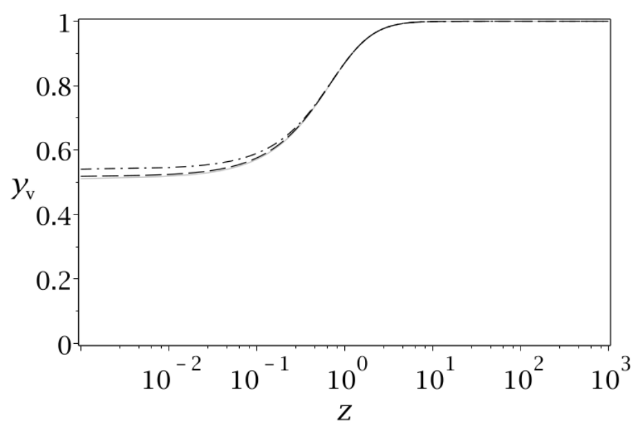
Historically the type of analytical approximation given in equation (70) can be traced back to Peebles [15], who gave it in the form as an approximation at the present time. For models containing negative curvature , a similar approximation was given by Lightman and Schester [11], with , see also [5]. Lahav et al. [10] realized that this type of approximations could be extended to general redshift , and they further refined it according to
| (72) |
where
| (73) |
Later Wang and Steinhardt [25], see also references therein, clarified that the values and are approximations to , obtained by the series expansion given in (70); see also [16] for the correct next order term in the exponent for CDM, which is given in equation (70). The approximations in equation (72), , and are quite good when compared with the explicit solution (63), as shown by plotting the errors , i.e. the difference between an approximation and the explicit solution (63), in figure 5(a). For another discussion about approximations, see [9]. Let us now introduce the following simple correction to , which compensates for the errors for the intermediate evolution,1717 17 Most of the approximations in this subsection are algorithmic in nature, but , and our new expression are not. In the dynamical systems setting they correspond to curve fitting, but all aim at approximating the full analytical growing mode solution of .
| (74) |
where the range of is determined by . As seen in figure 5(b), equation (74) is an approximation which is more accurate than by several orders of magnitude for all observational . It is possible to improve the accuracy further, but we have not been able to do so significantly with an approximation that is as simple or simpler than the present one. It should be noted that all approximations are quite good for large , i.e., small ; the differences reside in values for that are relevant for large scale structure formation at comparatively late times.
4 Tensor perturbations
Linear tensor perturbations of the spatially flat RW background geometry are characterized by a perturbed metric of the form
| (75) |
where is a gauge invariant that satisfies , . In the absence of anisotropic stresses the perturbed Einstein equations assume the following form (e.g. Malik and Wands (2009) [14], equation (8.6)):
| (76) |
This equation is now going to be used to illustrate the general discussion in section 2 in more detail. In order to formulate this equation as a dynamical system we first introduce -fold time, which yields
| (77) |
Using spatial Cartesian coordinates we apply the Fourier transform to this partial differential equation and write the transform of as a linear combination of time-independent polarization tensors and :1818 18 See, e.g., Weinberg (2008) [26], page 232 for more detail.
| (78) |
where is the wave number, and are complex-valued functions. The outcome is that each of the functions satisfy the following ordinary differential equation:
| (79) |
In the rest of this section the complex-valued function will denote either or and we will usually not indicate the dependence on the wave number explicitly. We finally specialize this differential equation to the CDM universe using (17b), (18) and, (20) to obtain
| (80) |
where we have introduced a scaled wave number according to .
The final step in constructing a dynamical system (a system of first order autonomous differential equations) is to follow the approach used for the density perturbation and introduce a (real-valued) quotient variable analogous to . However, since in (80) is complex and stands for one of the two functions , we must write , and where are four real-valued functions which independently satisfy (80). Then for any one of these four functions, which we simply denote by , we define
| (81) |
To complete the process we have to choose a suitable time function . Considerations of the temporally -dependent functions in the system of perturbative ODEs in order to obtain a regular dynamical system result in a different than for scalar perturbations, namely1919 19 Compare with (10) and (27).
| (82) |
We now calculate by differentiating (81) and using (80) and by differentiating (82). After expressing the coefficients in terms of using (20) and (82) we obtain
| (83a) | ||||
| (83b) | ||||
| where | ||||
| (83c) | ||||
| (83d) | ||||
Thus equation (83) describes a one-parameter family of real-valued analytic dynamical systems labelled by the parameter , which yields the long wavelength approximation when . The state space is again the infinite strip defined by , which is to be traversed twice in order to describe the global state space of and .
The structure of the orbits of this system is very similar to that of the system (35), with a monotonically increasing function and with the fixed points lying on the boundaries and . We note that the fixed points do not depend on the arbitrary parameter , since on the boundaries the function equals zero. When specialized to these boundaries the differential equation (44a) results in the following equations:
| (84a) | ||||
| (84b) | ||||
It follows that on the boundary the fixed points are given by
| (85a) | ||||||
| (85b) | ||||||
Linearization shows that the fixed point is a hyperbolic saddle and that a single orbit originates from and is future asymptotic to the boundary. This special orbit is approximated by
| (86) |
Next, linearization shows that the fixed point is a hyperbolic source, and hence a one-parameter family of orbits originates from . A series expansion in results in
| (87) |
where parameterizes the different orbits.
On the boundary the fixed points are as follows:
| (88a) | ||||||
| (88b) | ||||||
Linearization shows that the fixed point is a hyperbolic saddle that attracts a single orbit that is past asymptotic to . A series expansion in yields:
| (89) |
Finally, linearization shows that the fixed point is a hyperbolic sink, which implies that a one-parameter family of orbits is asymptotic to . A series expansion in results in
| (90) |
where parameterizes the different orbits.
The orbit structure for tensor perturbations for CDM cosmology for a variety of values of is illustrated in figure 6. Note that for large , i.e., , orbits start to circulate the state space at an intermediate stage of the evolution. This regime is approximately described by the short wavelength limit for dust, but eventually the cosmological constant starts to dominate and the future asymptotic limits for the orbits are the same for all values of , since the fixed points at are independent of .


The long wavelength limit corresponds to and yields an explicit solution for , which is most conveniently expressed by using
| (91) |
which results in
| (92) |
In this case there are two special orbits, one with going from to and one with , for which , going from to . The structure of the orbits in the long wavelength limit is illustrated in figure 7.


5 Measures of anisotropy: the shear and Weyl tensors
In this paper we have given a global analysis of the evolution of linear scalar and tensor perturbations of a CDM universe by formulating the perturbed Einstein equations as dynamical systems. In order to place this analysis in perspective we now consider the family of solutions of the Einstein equations whose matter content is dust and a cosmological constant. These solutions model a class of universes that generalize the CDM universe which is the unique model in this class that describes a completely isotropic universe with flat spatial geometry. We will thus refer to these universes as generalized CDM universes. Complete isotropy is characterized by the requirement that the shear tensor of the fluid congruence and the Weyl curvature tensor are zero, see e.g. [24] and references therein. From an observational point of view one is interested in universes in which the anisotropy is small, by which one means that the shear tensor and the Weyl tensor are small relative to the overall expansion of the universe, described by the Hubble scalar . We thus form dimensionless scalars by normalizing the contracted shear and Weyl tensors2020 20 One can decompose the Weyl tensor into an electric and magnetic part relative to a given timelike congruence, with spatial components denoted and , where is the three dimensional alternating symbol. One can form space-time scalars using as below, or spatial scalars using the electric and magnetic parts. with an appropriate power of the Hubble scalar :
| (93) |
There exists a number of results about the evolution of generalized CDM universes. First, as regards late times it has been shown that universes in this family that expand indefinitely approach the de Sitter model for an open set of initial conditions,2121 21 This class of cosmologies is labelled by eight arbitrary spatial functions, Lim et al. (2004) [13], page 8. in the sense that
| (94) |
Second it has been shown that there is a subset of models which approximate the flat RW (Friedmann-Lemaître) model on approach to the singularity,2222 22 This class of cosmologies is labelled by three arbitrary spatial functions [13], page 11.
| (95) |
The singularity in these models is referred to as an isotropic singularity (see Goode and Wainwright (1985) [7]). On the other hand a typical model undergoes a more complicated evolution described by BKL oscillations and possible so-called spike oscillations on approach to the singularity (see e.g. Uggla (2013) [18]). Nevertheless, the Hubble-normalized anisotropy scalars and remain bounded during this process, a result that we will use later in this section.
In this paper we have illustrated the global solution space of the linearly perturbed CDM models using dynamical systems that describe scalar and tensor perturbations separately. We will now use the shear and Weyl tensors to compare the asymptotic behaviour of the perturbations at early and late times with the full state space picture of Einstein’s field equations in the Hubble-normalized state space description given in [13], and briefly described above. The purpose with this is to shed light on the important issue of assessing the validity of cosmological linear pertubations as approximations to solutions of the Einstein field equations.
We refer to [19] for expressions for the perturbed shear and Weyl tensors.2323 23 See equations (B35a) and (B41c), which we specialize as follows. We assume zero anisotropic stress, which implies , a flat background () and for simplicity we exclude the vector mode (). Note that the present . For the linear scalar and tensor perturbations the perturbed shear tensor is given by
| (96a) | |||
| while the perturbed electric Weyl tensor is given by2424 24 One can give a similar expression for the perturbed magnetic Weyl tensor, but we have found that it has similar asymptotic properties as the electric Weyl tensor. | |||
| (96b) | |||
5.1 Scalar perturbations
Using the relations (61)
| (97) |
and the scalar mode extraction operator we form the Hubble-normalized shear and electric Weyl scalars for the scalar perturbations:2525 25 , where is the inverse spatial Laplacian, , and where spatial indices are raised with , see Appendix A in [20].
| (98a) | ||||
| (98b) | ||||
In the dynamical systems formulation for the scalar perturbations we have chosen a variable according to equation (27) which yields and
| (99) |
One can express and in the non-reduced state space , which yields
| (100) |
Using the previously obtained asymptotic expressions for , and inserting them into equation (30) for to obtain asymptotic expressions for , subsequently results in asymptotic expressions when and for and . However, since we in the present case have explicit solutions for and , given in equation (52), we can give explicit expressions for and as functions of :
| (101a) | ||||
| (101b) | ||||
where we recall that . It follows that
| (102) |
where the second result follows from when . The Weyl scalar has the same limits. One can also infer the asymptotic rate of growth/decay of and as from equation (101):
| (103) |
The limits (102) suggest that the growing mode (the orbit past asymptotic to the fixed point , given by ), approximates an exact solution with an isotropic singularity. The asymptotic decay rate in (103) agrees with the asymptotic results of Lim et al. (2004) [13] (see equations (4.19) and (5.9)). On the other hand, the unboundedness of the Hubble-normalized shear and Weyl perturbation when indicates that generic perturbations become physically unviable, i.e. they do not approximate exact solutions of the Einstein field equations, when is sufficiently close to zero (recall that investigations of the Einstein field equations indicate that the Hubble-normalized shear and Weyl tensors are expected to be bounded generically).
One can also use (101) to determine the asymptotic behaviour of and at late times (). Since is finite it follows that
| (104) |
for all . Equation (101) also gives the rates of decay along generic orbits asymptotic to the fixed point :
| (105) |
The result (104) for perturbations of CDM is compatible with the future asymptotic behaviour of generalized CDM universes toward a future de Sitter state, as described by equation (94), where equation (105) agrees with the asymptotic results of Lim et al (2004) [13] (see equations (3.24) and (5.8)).
5.2 Tensor perturbations
To analyze the tensor perturbations we make the transition (78) to Fourier space and use one of the four real-valued functions to represent the perturbation. Thus according to (96) the shear will be represented by and the electric Weyl tensor will be represented by , which motivates defining the shear scalar and electric Weyl scalar for tensor perturbations according to
| (106) |
where
| (107) |
In order to analyze the behaviour of these scalars along the orbits we first rewrite the defining equation in the form and then integrate to obtain
| (108) |
It then follows from (106) that and are given as functions of along the orbits by
| (109) |
We can now use the asymptotic expansions for the four fixed points in the previous section to determine the asymptotic form of and hence of . We first consider the orbits that are past asymptotic to and as , referring to equations (86) and (87):
| (110a) | |||||||||||||
| (110b) | |||||||||||||
One can further obtain the leading temporal -dependence, as follows:
| (111) |
Since it follows from (109) that has the same asymptotic behaviour as .
The above results describe the asymptotic behaviour of the perturbed shear and electric Weyl scalars near the initial singularity. The results are the same as for scalar perturbations. For example, only the single orbit in figure 6 and figure 7 is compatible with an isotropic singularity and this orbit is thus analogous to the growing mode orbit for scalar perturbations in figure 1. Also, analogously with the scalar perturbations, generically tensor perturbations result in unbounded Hubble-normalized shear and Weyl tensors, suggesting that the perturbations asymptotically are no longer approximations to the Einstein field equations when approaching toward the past.
We now consider the orbits that are future asymptotic to the fixed points and as , referring to equations (90) and (89):
| (112a) | ||||||||||||||
| (112b) | ||||||||||||||
One can further obtain the leading -dependence, as follows:
| (113) |
Again, has the same asymptotic behaviour as . Here there is one difference between the scalar and tensor perturbations: both and are as , while is and is . Since the asymptotic perturbations agree with the asymptotic results for the full Einstein equations in (94) one expects that the perturbations will approximate exact solutions at late times toward the future asymptotic de Sitter state.2626 26 As regards fluids with rotation, vector perturbations are given by , where depends on the spatial coordinates only, as follows from equation (58a) in [19]. Equations (58b), (42a), (66d) in the same reference yields , which together with when inserted into equation (B.41c) for the vector mode of results in that this quantity is when . Hence the vector mode has to be set to zero in the case of an isotropic singularity. Equation (B.41d) in [19] for the fluid rotation also results in an initial blow up, unless the vector mode is set to zero.
6 Concluding remarks
The purpose of this paper has been to develop a new approach to using dynamical systems methods to analyze linear perturbations on a spatially flat RW background. We decided to use the CDM model to illustrate the method because of its importance in cosmology and because of its relative mathematical simplicity. In our approach the state space of the dynamical system has a product structure
| (114) |
where is the background state space which describes the dynamics of the flat RW background, and is the perturbation state space, which contains the gauge invariant perturbation variables.
The Einstein equations in the RW background give a system of autonomous differential equations on and the linearly perturbed Einstein equations give a system of autonomous differential equations for the perturbation variables in , which involve the background variables in . In this way the dynamics in the background determine the dynamics of the perturbations. The advantage of the product structure is that when an orbit on is projected onto the background it coincides with an orbit on .
A key step is to choose bounded variables so that the state space is compactified and the system of autonomous differential equations is regular. It is also desirable to take advantage of the fact that the Einstein equations make it possible to decouple some of the variables, leaving a reduced state space to describe the essential dynamics.
The mathematical simplicity of the CDM model is reflected in the fact that it is possible to use only one background variable and one perturbation variable to describe the essential dynamics. In other words both and are one dimensional spaces. For example, in the case of scalar perturbations in the uniform curvature gauge we represented as the unit line segment with as the background variable, and as the circle described by the angular variable . The state space is thus which is a finite segment of a cylinder. Because the state space is bounded we were able to give a global description of the dynamics, in particular the behaviour at early and late times and the evolution at intermediate stages that may be of physical interest. In addition the differential equations, using fold time are well-suited for performing numerical simulations.
In future papers we will show how to obtain reduced and compactified product state spaces with systems of regular differential equations for scalar field models and models with multiple sources. As a first step we will consider the simplest case, namely a minimally coupled scalar field with exponential potential, for which is two dimensional and is one dimensional. This case will provide the basis for the generalization to the case of a scalar field with more general potentials, which requires that is three dimensional. This will also illustrate how one can organize perturbation theory into hierarchical structures where simpler models act as building blocks for more complicated ones.
Acknowledgments
AA is funded by the FCT grant SFRH/BPD/85194/2012, and supported by the project (GPSEinstein) PTDC/MAT-ANA/1275/2014, and CAMGSD, Instituto Superior Técnico by FCT/Portugal through UID/MAT/04459/2013. Furthermore, AA thanks the warm hospitality of Karlstad University. CU would like to thank the CAMGSD, Instituto Superior Técnico in Lisbon and the University of Waterloo, Canada, for kind hospitality.
References
- [1] M. Abramowitz and I.A. Stegun. Handbook of mathematical functions 10th ed. Dover Publications, 1972.
- [2] A. Alho and C. Uggla. Global dynamics and inflationary center manifold and slow-roll approximants. Journal of Mathematical Physics, 56(012502), 2015.
- [3] S. Basilakos, G. Leon, G. Papagiannopoulos, and E. N. Saridaki. Dynamical system analysis at background and perturbation levels: Quintessence in severe disadvantage comparing to lcdm. Phys. Rev. D, 100(4):043524, 2019.
- [4] M. Bruni and K. Piotrkowska. Dust - radiation universes: Stability analysis. Mon. Not. Roy. Astron. Soc., 270:630–640, 1994.
- [5] S. M. Carroll, W. H. Press, and E. L. Turner. The cosmological constant. Ann. Rev. Astron. Astrophys., 30:499–542, 1992.
- [6] Planck Collaboration. Planck 2018 results. VI. cosmological parameters. arXiv:1807.06209 [astro-ph.CO], 2018.
- [7] S. Goode and J. Wainwright. Isotropic singularities in cosmological models. Class. Quantum Grav., 2:99, 1985.
- [8] H. A. Gressel and M. Bruni. fnl - gnl mixing in the matter density field at higher orders. JCAP, (06):016, 2018.
- [9] A. J. S. Hamilton. Formulae for growth factors in expanding universes containing matter and a cosmological constant. Month. Roy. Astron. Soc., 322:419–425, apr 2001.
- [10] O. Lahav, P. B. Lilje, J. R. Primack, and M. J. Rees. Dynamical effects of the cosmological constant. Month. Roy. Astron. Soc., 251:128–136, jul 1991.
- [11] A. P. Lightman and P. L. Schechter. The omega dependence of peculiar velocities induced by spherical density perturbations. Astro. Phys. J., 74:831, dec 1990.
- [12] W. C. Lim. The dynamics of inhomogeneous cosmologies. 2004.
- [13] W. C. Lim, H. van Elst, C. Uggla, and J. Wainwright. Asymptotic isotropization in inhomogeneous cosmology. Phys. Rev., D69:103507, 2004.
- [14] K. A. Malik and D. Wands. Cosmological perturbations. Physics Reports, 475:1–51, 2009.
- [15] P. J. E. Peebles. The large-scale structure of the universe. Princeton University Press, 1980.
- [16] S. Tsujikawa, A. De Felice, and J. Alcaniz. Testing for dynamical dark energy models with redshift-space distortions. JCAP, 1301:030, 2013.
- [17] C. Uggla. Asymptotic cosmological solutions: orthogonal bianchi type-ii models. Class. Quantum Grav., 6(3):383, 1989.
- [18] C. Uggla. Recent developments concerning generic spacelike singularities. Gen. Rel. Grav., 45:1669–1710, 2013.
- [19] C. Uggla and J. Wainwright. Cosmological perturbation theory revisited. Class. Quantum Grav., 28:175017, 2011.
- [20] C. Uggla and J. Wainwright. A simplified structure for the second order cosmological perturbation equations. Gen. Rel. Grav., 45:643, 2013.
- [21] C. Uggla and J. Wainwright. Second order cosmological perturbations: dynamics. Phys. Rev. D, 98:103534, 2018.
- [22] C. Uggla and J. Wainwright. Second order cosmological perturbations: new conserved quantities and the general solution at super-horizon scale. Phys. Rev. D, 100(2):023544, 2019.
- [23] C. Uggla and J. Wainwright. Second order cosmological perturbations: simplified gauge change formulas. Class. Quantum Grav., 36:035004, 2019.
- [24] J. Wainwright and G. F. R. Ellis. Dynamical systems in cosmology. Cambridge University Press, 1997.
- [25] L. Wang and P. J. Steinhardt. Cluster abundance constraints for cosmological models with a time-varying, spatially inhomogeneous energy component with negative pressure. The Astrophysical Journal, 508(2):483, 1998.
- [26] S. Weinberg. Cosmology. Oxford university press, 2008.