On functions computed on trees
Abstract.
Any function can be constructed using a hierarchy of simpler functions through compositions. Such a hierarchy can be characterized by a binary rooted tree. Each node of this tree is associated with a function which takes as inputs two numbers from its children and produces one output. Since thinking about functions in terms of computation graphs is getting popular we may want to know which functions can be implemented on a given tree. Here, we describe a set of necessary constraints in the form of a system of non-linear partial differential equations that must be satisfied. Moreover, we prove that these conditions are sufficient in both contexts of analytic and bit-valued functions. In the latter case, we explicitly enumerate discrete functions and observe that there are relatively few. Our point of view allows us to compare different neural network architectures in regard to their function spaces. Our work connects the structure of computation graphs with the functions they can implement and has potential applications to neuroscience and computer science.
1. Introduction
A complicated function can be constructed by a hierarchy of simpler functions. For instance, when a microprocessor calculates the value of a function for a given set of inputs, it computes the function through composing simpler implemented functions, e.g. logic gates [HG91, GHR92]. Another example is that of an addition function for any number of inputs which can be obtained by composing simpler addition functions of two inputs. Even when the set of simple functions is small, like in the case of working only with logic gates, the set of functions that can be built may be exponentially large. We know from computation theory that all computable functions can be constructed in this manner [Sip06, AB09]. Therefore, one approach to understand the set of computable functions is to investigate their potential representations as hierarchical compositions of simpler functions.
Here we study the set of functions of multiple variables that can be computed by a hierarchy of functions that each accepts two inputs. Such compositions can be characterized by binary rooted trees (in the following we will refer to them as binary trees) that determines the hierarchical order in which the functions of two variables are applied. Associated with any binary tree is a (continuous or discrete) tree function space (TFS) consisting of all functions that can be obtained as a composition (superposition) based on the hierarchy that the tree provides. In Theorem 2.2 we exhibit a set of necessary and sufficient conditions for analytic functions of variables to have a representation via a given tree. We show that this amounts to describing the corresponding TFS as the solution set to a group of non-linear partial differential equations (PDEs). We also study the same representability problem in the context of discrete functions.
Related mathematical background. Representing multivariate continuous functions in terms of functions of fewer variables has a rich background that roots back to the problem on David Hilbert’s famous list of mathematical problems for the century [Hil02]. Hilbert’s original conjecture was about describing solutions of degree equations in terms of functions of two variables. The problem has many variants based on the category of functions – e.g. algebraic, analytic, smooth or continuous – in which the question is posed. See [VH67, chap. 1] or the survey article [Vit04] for a historical account. Later in the 1950s, the Soviet mathematicians Andrey Kolmogorov and Vladimir Arnold did a thorough study of this problem in the context of continuous functions that culminated in the seminal Kolmogorov-Arnold Representation Theorem ([Kol57]) which asserts that every continuous function can be described as
| (1.1) |
for suitable continuous single variable functions , .11
1
There are more refined versions of this theorem with more restrictions on the single variable functions that appear in the representation [Lor66, chap. 11]. So in a sense, addition is the only real multivariate function. The idea of applying Kolmogorov-like results to studying networks is not new. Based on the mathematical works of Anatoli Vituškin (see below), the article [GP89] argues that to quantify the complexity of a function, its number of variables (not a suitable indication of the complexity due to Kolmogorov-Arnold Theorem) must be combined with the degree of smoothness due to the fact that there are highly regular functions that cannot be represented by continuously differentiable functions of a smaller number of variables [Vit54]. The paper then concludes that it is not possible to obtain an exact representation usable in the context of network theory because of this emergence of non-differentiable functions. Nevertheless, the article [Ků91] argues that there is an approximation result of this type.
Although pertinent to our discussion, the reader should be aware that the representations of multivariate functions studied in this article are different in following ways:
- •
Motivated by both the structures of computation graphs and the model of neurons as binary trees, we desire multivariate functions that could be obtained via composition of functions of two variables instead of single variable ones.
- •
Unlike the summation above, we work with a single superposition of functions. In the presence of differentiability, this enables us to use the full power of the chain rule. In the case of ternary functions for instance, a typical question (to be addressed in §5.1) would be whether can be written as . In fact, if one allows sum of superpositions, a result of Arnold (which could be found in his collected works [Arn09b]) states that every continuous can be written as a sum of nine superpositions of the form . But we look for a single superposition, not a sum of them.
- •
We mostly work in the analytic context; see §5.3 for difficulties that may arise if one works with smooth functions. It must be mentioned that assuming that the continuous has certain regularity (e.g. smooth or analytic) does not guarantee that in a representation such as (1.1) the functions can be arranged to be of the same smoothness class [Vit64]. In fact, it is known that there are always functions22 2 A function is called (of class) if it is differentiable of order and its order partial derivatives are continuous. A () function is said to be (resp. times) continuously differentiable. A function which is infinitely many times differentiable is called smooth or (of class) . The smaller class of (real) analytic functions that are locally given by convergent power series is denoted by . We refer the reader to [Pug02] for the standard material from elementary mathematical analysis. of three variables which cannot be represented as sums of superpositions of the form with and being as well [Vit54]. Because of the constraints that we put on in our main result, Theorem 2.2, it turns out that the functions of two variables that appeared in tree representations are analytic as well, or even polynomial if is polynomial; see Proposition 5.9.
- •
Applying the chain rule to superpositions of analytic (or just ) bivariate functions results in the PDE constraints (2.4). It must be mentioned that the fact that the partial derivatives of functions appearing in any superposition of differentiable functions must be related to each other is by no means new. Hilbert himself has employed this point of view to construct analytic functions of three variables that are not (single or sum of) superpositions of analytic functions of two variables [Arn09a, p. 28]. Ostrowski for instance, has used this idea to exhibit an analytic bivariate function that cannot be represented as a superposition of single variable smooth functions and multivariate algebraic functions due to the fact that it is not a solution to any non-trivial algebraic PDE [Ost20], [Vit04, p. 14]. But, to the best of our knowledge, a systematic characterization of superpositions of analytic bivariate functions as outlined in Theorem 2.2 (or its discrete version in Theorem 6.6) and utilizing that for studying tree functions and neural networks has not appeared in the literature before.
Neuroscience motivation. Over a century ago, the father of modern neuroscience, Santiago Ramón y Cajal, drew the distinctive shapes of neurons [yC95]. Neurons receive their inputs on their dendrites which both exhibit non-linear functions and have a tree structure. The trees, called morphologies, are central to neuron simulations [HC97, Rei99]. Neuronal morphologies are not just the distinctive shapes of neuron but also pertain to their functions. One approximate way of thinking about neural function is that neurons receive inputs and by passing from the dendritic periphery towards the root, the soma, implement computation which gives a neuron its input-output function. In that view, the question of what a neuron with a given dendritic tree and inputs may compute boils down to the question of characterizing its TFS.
The paper is organized as follows. §2 is devoted to a detailed outline the paper. We also state the main results after a non-technical motivation. In §3 we discuss the relevant literature from both computer science and neuroscience sides of the theory. Several possible extensions and open problems are stated as well. The central concept of this paper, tree functions, is formally defined in §4. Sections 5 and 6 treat tree functions in analytic and bit-valued contexts respectively. Finally, in §7 we apply these ideas to study neural networks via tree functions.
2. Outline and overview of main results
The order of appearance of functions in a superposition can be represented by a tree whose leaves, nodes (branch points) and root represent inputs, functions occurring in the superposition and the output respectively. Here we assume that the tree and the set of functions that could be applied at each node are given and each leaf is labeled by a variable. We can now define the space of functions generated through superposition, i.e. the corresponding tree function space (TFS) (see Definition 4.1). The most tangible case of a TFS is when all of the inputs are real numbers and the functions assigned to the nodes are bivariate real-valued functions. Nonetheless, our definition in §4 covers other cases: an arbitrary tree and sets of functions associated with its nodes result in the set of functions represented by superpositions. One example is when the functions at the nodes are bit-valued functions. Another example is when the inputs are time-dependent and the functions at nodes are operators. The latter case is important since it contains the function that a neural morphology would implement when we only allow soma-directed influences and ignore back-propagating action potentials [SSSH97].
The smallest non-trivial tree representing a superposition is the one with three leaves illustrated in Figure 1(b). Denoting the inputs by , and , an element of the corresponding TFS is the superposition below of a function of two variables and :
| (2.1) |
For and multiplication or addition, we end up with two basic examples and . By changing and one can construct other examples and hence the question of which functions could be answered in this manner.
To find a necessary condition for a function of three variables to have a representation such as (2.1), we assume differentiability and take the derivative. A straightforward application of the chain rule to (2.1) shows that must satisfy
| (2.2) |
A detailed treatment may be found in the discussion from the beginning of §5.1. This partial differential equation for puts a constraint on functions in the TFS and hence rules out certain ternary functions such as
| (2.3) |
While (2.2) is only a necessary condition, we prove that it is also sufficient in the case of analytic () functions:
Proposition 2.1.
Let be an analytic function defined on an open neighborhood of the origin that satisfies the identity in (2.2). Then there exist analytic functions and for which over some neighborhood of the origin.
To prove Proposition 2.1, we look at the Taylor expansion of with respect to and argue that each partial derivative has a representation like (2.1). We then explicitly construct the desired and in (2.1) with the help of the Taylor series. Consequently, we arrive at a description of the TFS containing analytic functions of three variables as the set of solutions to a single PDE.

Generalizing this setup to a higher number of variables, the following question arises: When can an analytic multivariate function be obtained from composition of functions of two variables? Allowing more than three leaves results in graph-theoretically distinct binary trees. For example, in the case of functions of four variables, there exist two non-isomorphic binary trees; Figure 1. The corresponding representations are
for the first tree and
for the second one. Thus each (labeled) binary tree comes with its corresponding space of analytic tree functions that could be obtained from analytic functions on smaller number of variables via composition according to the hierarchy that provides; see Definition 4.1.
Condition (2.2) from the ternary case is the prototype of constraints that general smooth functions from a TFS must satisfy. By fixing variables of a function of variables in the TFS under consideration, the resulting function of three variables belongs to the TFS of the tree formed by those three leaves and is hence a solution to a PDE of the form (2.2). Since this is true for any triple of variables, numerous necessary conditions must be imposed. In Theorem 2.2 we prove that for analytic functions, these conditions are again sufficient.
Theorem 2.2.
Let be a binary tree with terminals and . Suppose the terminals of are labeled by the coordinate functions on . Then for any three leaves of corresponding to variables of with the property that there is a sub-tree of containing the leaves while missing the leaf (Figure 2)33 3 Clearly, there is always a rooted sub-tree that separates one of the leaves from the other two: consider the smallest rooted sub-tree (cf. §4 or Figure 6 for the terminology) that has all of them as leaves. Adjacent to the root of this smaller binary tree are its left and right sub-trees. One of them must contain two of and the other one has the third leaf., must satisfy
| (2.4) |
Conversely, an analytic function defined in a neighborhood of a point can be implemented on the tree provided that for any triple of its variables with the above property (2.4) holds and moreover, for any two sibling leaves , either or is non-zero.


The general argument for the trees with larger number of leaves builds on the proof in the case of ternary functions demonstrated above. The proof occupies §5.2 and heavily uses the analyticity assumption. We digress to the setting of smooth () function in §5.3 to show that this assumption cannot be dropped.
The constraints in the Theorem 2.2 are algebraically dependent. The number of the constraints imposed by Theorem 2.2 is , hence cubic in the number of leaves. In §5.4 we show that “generically” the number of constraints could be reduced to . This leads to a heuristic44 4 We use the term “heuristic” both because the space of analytic functions that Theorem 2.2 deals with is infinite-dimensional and so one should be careful about the exact meaning of co-dimension; and moreover, because the number of constraints is not necessarily synonymous to the deficit of the dimension of the subspace of tree functions. This is because each constraint in the form of (2.4) is a functional identity that could amount to multiple constraints on the coefficients of the Taylor expansion. result on the co-dimension of the TFS in Proposition 5.6 which states that the number of independent functional equations describing a TFS grows only quadratically with the number of leaves.
The space of analytic functions is infinite-dimensional and this makes it difficult to rigorously measure how “small” a TFS is relative to the ambient space of all analytic functions. However, under certain restrictions, the dimensions of the tree function space or even the space itself are finite. Two examples are worthy of investigation: bit-valued functions of the form and polynomials of bounded degree. In the bit-valued setting of §6.1 each node is characterized by a function . We prove that Theorem 2.2 still holds in the sense of formal differentiation; see Theorem 6.6. Moreover, we enumerate the functions in the discrete TFS as (Corollary 6.2), a number which is much smaller than the number of all possible bit-valued functions which is . We use this to conclude that the total number of tree functions of variables obtained from all labeled binary trees of leaves is ; see Corollary 6.3. In the polynomial setting, each node is a bivariate polynomial. We establish that the Theorem 2.2 applies and furthermore, holds globally; cf. Proposition 5.9. In this case, if we consider polynomials of variables and of degree not greater than , the polynomial TFS would be of an algebraic variety whose dimension does not exceed ; see Proposition 5.11. Again, observe that this is much smaller than the dimension of the ambient polynomial space.
The set of binary functions that can be implemented on a given tree is limited and this set allows the reconstruction of the underlying tree from its corresponding TFS; see Proposition 6.9. For two labeled trees we define a metric: the proportion of functions that can only be represented by one of the trees (§6.2). This can be useful: in the case of two neurons with different morphologies, this simple metric quantifies how similar the sets of functions are that the two neurons can implement.

In a more general manner, the functions defined by neural networks are interesting examples of superpositions. In §7.1 we discuss a procedure of “expanding” a neural network to a tree by forming the corresponding Tree Expansion of the Neural Network or TENN for short. The idea is to convert the neural network of interest into a tree by duplicating the nodes that are connected to more than one node of the upper layer; see Figure 4. The procedure then allows us to revert back to the familiar setting of trees. A crucial point to notice is that, unlike previous sections, trees associated with neural networks are not necessarily binary and furthermore, a variable could appear as the label of more than one leaf. In other words, the functions constituting the superposition may have variables in common, e.g. . Seeking similar constraints for describing the TFS of a tree with repeated labels, in §7.2 we take a closer look at the preceding superposition to obtain a necessary condition:
Proposition 2.3.
Assuming that are four times differentiable, the superposition satisfies the PDE below:
The proposition suggests that tree functions are again solutions to (perhaps more tedious) PDEs. It is intriguing to ask if in presence of repeated labels there is a characterization, similar to Theorem 2.2, of a TFS as the solution set to a system of PDEs; cf. Question 7.2. We finish with one final application of this idea of transforming a neural network to a tree: In Theorem 7.9 of §7.3, we give an upper bound on the number of bit-valued functions computable by a neural network in terms of parameters depending on the architecture of the network.
3. Discussion
Here we study the functions that are obtained from hierarchical superpositions; we study functions that can be computed on trees. The hierarchy is represented by a rooted binary tree where the leaves take different inputs and at each node a bivariate function is applied to outputs from the previous layer. In the setting of analytic functions, in Theorem 2.2 we characterize the space of functions that could be generated accordingly as the solution set to a system of PDEs. This characterization enables us to construct examples (e.g. (2.3)) of functions that could not be implemented on a prescribed tree. This is reminiscent of Minsky’s famous XOR theorem [MP17]. The space of analytic functions is infinite-dimensional and this motivates us to investigate two settings in which the TFS is finite-dimensional (polynomials) or even finite (bit-valued). We show that the dimension or size of the TFS is considerably smaller than that of the ambient function space. The number of bit-valued functions could be estimated even for non-binary trees following the same ideas. Finally, we bridge between trees and neural networks by associating with each feed-forward neural network its corresponding TENN; cf. Figure 4. This procedure allows us to apply our analysis of trees yielding an upper bound for the number of bit-valued functions that can be implemented by a neural network.
Our main result in the continuous setting, Theorem 2.2, holds only for analytic functions; see the discussion in §5.3. While they constitute a large class of functions, there are important cases where one must deal with continuous non-analytic functions too. For example, a typical deep learning network is built through composition from analytic functions such as linear and sigmoid functions or the hyperbolic tangent; and also, from non-analytic functions such as ReLU or the pooling function. Continuous functions could be approximated locally by analytic ones with any desired precision (although not over the entirety of the real axis). Therefore, while our main result (local by formulation) is an exact classification, one future direction is to study how well arbitrary continuous functions could be approximated by analytic tree functions.
The morphology of the dendrites of neurons processes information through a (commonly binary [KD05, GA15]) tree and so it is naturally related to the setup of this paper; see Figure 5 [Mel94, PBM03]. A typical dendritic tree receives synaptic inputs from surrounding neurons. When activated, the synapses induce a current which changes the voltage on the dendrite. This is followed by a flow of the resulting current towards (and away from) the root (soma) of the neuron. In typical models of neural physiology, a neuron is segmented into compartments where their connections and the biological parameters define the dynamics of the voltage for each compartment [Seg98]. The dynamics of the electrical activity is often given by the following well-known ODE55 5 The quantities appeared here are: • is the voltage potential of the compartment; • is the resting voltage potential for the compartment and the ion ; • is the membrane capacitance of the compartment; • denotes the resistance of the compartment and is the resistance between and compartments; • is non-linear function corresponding to the ion . We only consider currents towards the soma. [HC97]:
| (3.1) |
Consequently, in the case of time-varying inputs, TFSs could be of neuroscientific interest. In this situation, the functions at the nodes are operators that receive time-dependent functions as their inputs. Constraints such as (2.4) in the main theorem may be formulated in this case as well: An operator
admitting a tree representation is expected to satisfy equations such as
| (3.2) |
where derivatives of the operator must be understood in the variational sense
Utilizing discrete TFSs, in §6.2 we introduce a metric on the set of labeled binary trees that may be potentially used to quantify how similar two neurons are. A careful adaptation of our results to the time-varying situation could be the object of future enquiries.
Certain assumptions must be made before any application of our treatment of tree functions to the study of neural morphologies. First, from a biological standpoint not all functions are admissible as functions applied at nodes of neurons. Secondly, the acyclic nature of trees assumes that a neuron functions only due to feed-forward propagation whereas in reality back-propagating action potentials also occur. Thirdly, it is well-known that there are biological mechanisms, such as ephaptic connectivity or neuromodulations, that could affect the computations in a neuron’s morphology, and they are not taken into account in typical compartmental models. Our approach only applies to an abstraction of models; however, this abstraction appears meaningful.

In this paper, the “complexity” of a TFS in bit-valued and polynomial settings is measured by its cardinality or dimension. However, there are other notions of complexity in the literature that try to capture the capacity of the space of computable functions. For example, the VC-dimension measures the expressive power of a space of functions by quantifying the set of separable stimuli [VLC94, ZP96, MLP17]. For linear combinations of smooth kernels, the minimum number of bases can measure the complexity of a classifier [BDLR05, BDR06]. This suggests that large complexities of shallow networks might be due to the “amount of variations” of functions to be computed [KS16]. When the functions at the nodes are piece-wise linear, one can count the number of linear regions of the output function [MPCB14, HR19]. The choice of the complexity measurement method is important when it comes to quantifying the difference between two architectures.
When a model is trained on data, we search for the best fit in the function space. Characterizing the landscape of function space can present new methods for training [BRK19]. To train models in machine learning, we use a variety of methods such as (stochastic) gradient decent, genetic algorithms, or more recent methods such as learning by coincidence [SL18]. For some models such as regression, we have explicit formulae that show how to find the parameters from training data. One future line of research is to investigate whether our PDE description of the TFSs can point toward new methods of training.
Since a TFS is much smaller than the ambient space of functions, it is suggestive to consider the approximation by them. In this regard, we fix a target function and take into account the tree functions that approximate it. Searching for the best approximation of a target function in the function space is realized by the training process. Hence one important question for approximation of a function is the stability of this process [HR17]. Another approach is to develop the mean-field equations to approximate the function space with a fewer equations that are easier to handle [MMN18]. Poggio et al. have found a bound for the complexity of a neural networks with smooth (e.g. sigmoid) or non-smooth (e.g. ReLU) non-linearity that provides a prescribed accuracy for functions of a certain regularity [PMR+17]. Also by estimating the statistical risk of a neural network, one can describe model complexity relative to sample size [BK18]. Now that we have a description of analytic tree functions as solutions to a system of PDEs, one further direction is to study approximations of arbitrary continuous functions by these solutions.
When the tree function is fed the same input more than once through different leaves, the constraints put on superpositions in Theorem 2.2 must be refined and become more tedious. In §7.2, we study the simplest possible case, namely the superposition (7.1). Computing higher derivatives via the chain rule along with a linear algebra argument yield the complicated fourth order PDE of Proposition 2.3 as a constraint. One future line of research is to formulate similar PDE constraints in the case of general (not necessary binary) trees with repeated labels; cf. Question 7.2. Finding necessary or sufficient constraints in the repeated regime would have immediate applications to the study of continuous functions computed via neural networks with this consideration in mind that for the TENN associated with a neural network even functions assigned to nodes are probably repeated. Moreover, in the more specific context of polynomial functions, it is promising to try to formulate results such as Proposition 5.11 about the space of polynomial tree functions; or in the bit-valued setting, any strengthening of the bound on the number of bit-valued functions implemented on a general tree that Corollary 7.7 provides would be desirable.
One major goal of the theoretical deep learning is to understand the role of various architectures of neural networks. Previous studies have shown that, compared to shallow networks, deep networks can represent more complex functions [BS14, LTR17, KS17]. Comparing VC-dimension of different architectures is insightful into why high-dimensional deep networks trained on large training sets often do not seem to show overfit [MLP17]. Theorem 7.9 from the last section of this paper provides further intuition in this direction once instead of more traditional fully connected multi-layer perceptrons, we work with currently more popular sparse neural networks (e.g. convolutional neural networks). This is due to the fact that in the tree expansion of a sparse network the number of children of any arbitrary node would be relatively small. Theorem 7.9 indicates that the number of bit-valued functions computable by the network could be large only if the associated tree has numerous leaves. Since the tree is sparse, this could happen only if the depth of the tree (or equivalently, that of the network) is relatively large. The discussion in §7 suggests that studying tree functions could serve as a foundation for interesting theoretical approaches to the study of neural networks.
4. Tree functions
In this section we define the function space associated with a tree in the most general setting. Suppose we have inputs (leaves) of a binary tree . We recursively compute the output by applying at each node a function and passing the result to the next level. These calculations continue until we reach the root.
Definition 4.1.
Let be a tree and the set of all possible inputs that a leaf could receive. For any , suppose . The tree function space, , is defined recursively: if has only one vertex. For larger trees, assuming that the successors of the root of are the roots of smaller sub-trees , define:
Tree function spaces could be investigated in two different regimes:
Definition 4.2.
A tree is called binary if every non-terminal vertex (every node) of it has precisely two successors; cf. Figure 6.
The terminology of binary trees.
- •
Root: the unique vertex with no predecessor/parent.
- •
Leaf/Terminal: a vertex with no successor66 6 The reader is cautioned that in our usage of terms such as “children”, “parent”, “successor” and “predecessor” in reference to vertices we have a rooted tree as illustrated in Figure 6 in mind where the root precedes every other vertex whereas to implement a function, the computations are done in the “upward” direction starting from the leaves in the lowest level and culminating at the root./child.
- •
Node/Branch point: a vertex which is not a leaf, i.e. has (two) successors.
- •
Sub-tree: all descendants of a vertex along with the vertex itself.
- •
Sibling leaves: two leaves with the same parent.
- •
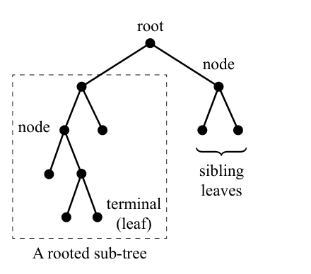
Convention. All trees are assumed to be rooted. The number of leaves (terminals) of a tree is always denoted by , and each leaf presents a variable. Unless stated otherwise, the tree is binary and these variables are assumed to be distinct, and hence the corresponding functions are of variables. Repeated labels come up only in §7.
5. Analytic function setting
5.1. The case of ternary functions
In this section, we focus on the first interesting case, namely a binary tree with three inputs. It turns out that the treatment of this basic case and the ideas therein are essential to the proof of Theorem 2.2. In order to make one output, two of the inputs should be first combined at one node, and the result of that combination is then combined with the third input at the root. Such functions can be written as:
| (5.1) |
where and are two smooth functions of two variables.
So which functions of three inputs, could be written as in (5.1)? Taking the derivative w.r.t. and , we have:
Taking the derivative w.r.t. yields:
Hence for every we should have:
| (5.2) |
as both sides coincide with . In particular, for
which is the constraint (2.2) from §2. Notice that the identity is solely based on the function and serves as a necessary condition for the existence of a presentation such as (5.1) for .
It is essential to observe that constraint (2.2) implies the rest of the constraints imposed on in (5.2). This is trivial for the points where . Otherwise, either or should be non-zero at the point under consideration and hence throughout a small enough neighborhood of it. We proceed by induction on . Differentiating (5.2) w.r.t. yields:
We claim that the latter terms of two sides coincide and this will finish the inductive step. From the induction hypothesis , while the base case indicates . The vectors and are multiples of the non-zero vector ; so they are multiples of each other, i.e. .
In the same vein, identity (2.4) implies the more general identity below:
| (5.3) |
This is true even for a greater number of variables in place of in the following sense:
Lemma 5.1.
Proof.
We next argue that locally, the aforementioned condition is sufficient. In another words, if an analytic ternary function satisfies (2.2), then it locally admits a tree representation such as (5.1).
Proof of Proposition 2.1.
Let us first impose a mild non-singularity condition at the origin: either or is non-zero. Without any loss of generality, we may assume and . The idea is to come up with a new coordinate system
| (5.4) |
centered at the origin in which the function is dependent on only . Define
| (5.5) |
The Jacobian of w.r.t. is given by
| (5.6) |
whose determinant at the origin is which we have assumed to be non-zero. Thus is indeed a coordinate system centered at . Next, we consider the Taylor expansion of w.r.t. :
| (5.7) |
the equality which holds near the origin due to the analyticity assumption. We claim that in the new coordinate system the partial derivatives that appeared above are independent of . The latter is clear and for the former we apply the chain rule to differentiate with respect to :
To calculate one has to invert the Jacobian matrix (5.6):
that yields . Plugging in the previous expression for we get:
which is zero due to (5.2); keep in mind that in a neighborhood of the origin the aforementioned identities are implied by (2.2); cf. Lemma 5.1. We conclude that in (5.7) each term is a function of , e.g.
Now defining to be and to be , the identity (5.7) implies that throughout a small enough neighborhood of .
Next, we omit the assumption that one of the partial derivatives of is non-zero in Proposition 2.1. If either of or is non-zero for some integer , we apply what we just proved to to get:
| (5.8) |
Then integrating times w.r.t. provides us with a similar expression for . There is nothing to prove if all of the partial derivatives and are zero since in that case the Taylor expansion of describes it as the sum of a function of and a function of . ∎
Remark 5.2.
The idea from the last part of the proof seems to work only for this particular presentation as in general, integration w.r.t. to one of the variables does not preserve forms such as . Therefore, we are going to need the non-singularity condition of Theorem 2.2 in the following section.
Remark 5.3.
An elegant reformulation (from the field of integrable systems) of constraint (2.2) imposed on a smooth tree function is to say that the differential form77 7 The reader may find a very readable account of the theory of differential forms on Euclidean spaces in [Pug02, chap. 9, sec. 5]. must satisfy :
Similar identities also hold in the general case of a (smooth) tree function as has appeared in Theorem 2.2. To any two sibling leaves assign the differential -form . A straightforward calculation yields as
which turns out to be zero since any other leaf is an outsider with respect to neighboring ; hence the terms inside parentheses vanish due to (2.4). The non-vanishing condition of Theorem 2.2 implies that these -forms are linearly independent throughout some small enough open subset of . They define a differential system on the aforementioned open subset whose rank is:
and the identities could be reinterpreted as the integrability of this system according to a classical theorem of Frobenius [Nar68, Theorem 2.11.11].
The discussion in this subsection settles Theorem 2.2 for the most basic case of a binary tree with three leaves.
5.2. Proof of the main theorem
Let be a binary tree with leaves as in Theorem 2.2 and be a differentiable function of variables on an open neighborhood of .
The proof of necessity
Let . Consider a triple of variables as in Theorem 2.2. For the ease of notation, suppose they are the first three coordinates . Given and a point
we need to verify (2.4) at . Setting the last coordinates to be constants we end up with the function
of three variables defined on the open neighborhood of which is the image of under the projection onto the first three coordinates . This new function is implemented on a tree with three inputs (corresponding to leaves in the original statement of Theorem 2.2) and with adjacent to the same node as and were separated from in the original tree; see Figure 3. Hence (2.2) holds for this function:
which at yields the desired constraint

Next, we argue that under the assumptions outlined in the second part of Theorem 2.2 the identities such as (2.4) are enough to implement on locally around . The proof of sufficiency is based on recursively constructing the desired presentation of as a composition of bivariate functions by reducing the size of . The base of the induction, the case of a tree with three terminals, has already been settled in Proposition 2.1.
We claim that, up to relabeling variables, can be written as either
| (5.9) |
or
| (5.10) |
where the function satisfies the hypothesis of the existence part of Theorem 2.2 for or variables (the integer is going to be introduced shortly). In terms of the tree , the first normal form occurs when is connected directly to the root; the removal of the leaf and the root then results in a smaller tree with leaves; cf. part (a) of Figure 7. The induction hypothesis then establishes and finishes the proof. On the other hand, (5.10) comes up when neither of the two rooted sub-trees obtained from excluding the root is singleton. The number here denotes the number of the leaves of one of these sub-trees, e.g. the “left” one. By symmetry, let us assume that variables are labeled such that are the leaves of the sub-tree to the left of the root while appear in the sub-tree to the right. Graph-theoretically, gathering the variables together in (5.10) amounts to collapse the left sub-tree to a leaf. This results in a new binary tree with the same root but with leaves which is of the form discussed before: it has a “top” leaf directly connected to the root; see part (b) of Figure 7. The final step is to invoke the induction hypothesis to argue that in (5.10) belongs to .
Part I of the proof of sufficiency: Suppose there is a leaf adjacent to the root.
Without loss of generality, we consider everything in a neighborhood of and assume .
Theorem 2.2 also requires at least one of the partial derivatives of w.r.t. to be non-zero; by symmetry, let us assume
.
Next, define
| (5.11) |
This is a new coordinate system centered at the origin as the Jacobian
| (5.12) |
is of determinant at the origin. The goal is to write down in a form
| (5.13) |
similar to (5.9) for a suitable bivariate function and then applying the induction hypothesis to which of course satisfies (2.4) with the original tree replaced with . To this end, we consider the Taylor expansion of w.r.t. :
| (5.14) |
We claim that the functions
appeared as coefficients are dependent only on the first component of the new coordinate system (5.11), or in other words
This is immediate when as we are basically differentiating w.r.t. . For , we need to apply the chain rule to get
where the partial derivatives are entries of the inverse of (5.12) given by
Hence is non-zero only for and
| (5.15) |
which is zero as (5.3) holds (keep in mind that the sub-tree of has while it misses since, as part (a) of Figure 7 demonstrates, the leaf corresponding to is connected directly to the root of .). Consequently, the term in (5.14) can be written as a function where has been defined to be in (5.11). Hence
works in (5.13). ∎
Part II of the proof of sufficiency: Suppose there is no leaf adjacent to the root.
We work with the convention discussed above: Among the two rooted sub-trees resulting from excluding the root of , the “left” one has variables as its leaves while the “right” one has the rest of the variables . The number is assumed to be larger than as the case of has just been treated in Part I of the proof of sufficiency.
Expand w.r.t. the last variables:
| (5.16) |
The non-vanishing assumption of Theorem 2.2 requires the partial derivative at of with respect to at least one of the variables in the left sub-tree to be non-zero; let us assume . By a similar Jacobian determinant computation appeared in part I of the proof, the assignment
| (5.17) |
defines a coordinate system centered at the origin of as . Repeating the argument that has come up multiple times before, the term
appeared in (5.16) is a function of since for every its derivative w.r.t. the component of the system (5.17) is zero due to
the identity that follows from Lemma 5.1 because the right sub-tree separates from the leaves of the left sub-tree. Therefore, (5.16) can be rewritten as
| (5.18) |
where the single variable function satisfies
| (5.19) |
The goal is to show that the function
| (5.20) |
of variables can be represented by the tree as in that case
is given by
which is in the form of (5.10) with obviously satisfying the induction hypothesis for the sub-tree to the left of the root and satisfying the same but for the tree with terminals obtained from collapsing the aforementioned left sub-tree of to a point. To verify the conditions of the theorem for , first observe that for the identity
holds trivially. This is due to the fact that by definition
| (5.21) |
which yields
| (5.22) |
for any and besides, satisfies the analogous constraint
It needs to be mentioned that furthermore, the non-vanishing requirement of the induction hypothesis can be deduced from (5.22) since
for every ; and any leaf of the new tree having a sibling leaf has to come from the original tree ; hence the desired
is the same as the non-vanishing condition
that the theorem has imposed on . Consequently, the challenging part would be to verify
| (5.23) |
for any . Differentiating (5.21) along with the definition of as yield
In particular, near the origin where , one has
| (5.24) |
Taking the partial derivatives of (5.24) w.r.t. variables (where ) and invoking (5.22), we see that (5.23) amounts to
which holds since
that is, one of the constraints imposed on in (2.4) ( is separated from via the right sub-tree). ∎
5.3. Smooth function setting
The proof above heavily relied on the analyticity of the function under consideration. As a matter of fact, in the context of functions one needs to strengthen the constraint (2.4) as follows (for simplicity, we have replaced , and with , and respectively):
| (5.25) |
for any two points and lying in an open ball on which is defined. This is best demonstrated for the superposition
from (5.1): The computations carried out there give us
which readily implies
Notice that the stronger constraint (5.25) could be derived from the ordinary ones (2.4) and (5.3) if the function is analytic: Form the single variable function
defined on an open interval of -values containing both and . The function vanishes at and we wish to show that it is identically zero as then it would be zero for too. Due to analyticity, it suffices to show that the derivatives of all orders vanish at . Notice that the derivative at that point is
which is zero due to (5.3). We are going to continue to work in the analytic category hereafter and so there would be no need to generalize constraint (2.4) to identities such as (5.25).
Example 5.4.
A typical example of a non-analytic smooth function is
We are going to use it to construct a smooth (but of course non-analytic) function of three variables that satisfies constraint (2.2) but not the generalized one introduced above. Set
We have
while
which coincide since they are both identically zero due to the fact that , and therefore , vanishes at non-positive numbers. Notice that the generalized condition is not satisfied here:
is positive when whereas
is zero in that case. It should not be surprising that in the absence of analyticity, serves as a counter example to Proposition 2.1: We are going to argue that there is no representation
of in a neighborhood of the origin with continuous functions of two variables. Aiming for a contradiction, suppose there are continuous functions satisfying
for where . Plugging and , we arrive at:
In conjunction, these two identities imply that is injective. This is absurd as for obvious topological reasons, there is no continuous injective map from any non-degenerate square to the real line.
5.4. Reducing the number of constraints
Theorem 2.2 provides necessary and sufficient conditions for a multivariate function to belong to the function space associated with a tree. Here, we approach the problem of finding the co-dimension of this infinite-dimensional subspace by counting the number of independent constraints. In general, the condition (2.2) of Theorem 2.2 should hold for any triple of variables and therefore, equations for a tree with leaves. However, many of these equations are redundant. To find the number of algebraically independent equations we shall need the following lemma.
Lemma 5.5.
Let be a binary tree. Denote its left and right sub-trees by and suppose that they have and leaves. Then the number of algebraically independent equations corresponding to triples that have elements from both and is .
Proof.
Denote the leaves of by and those of by . For the ease of notation, we switch to the subscript notation for partial derivatives. If is another leaf of (different from ) and is another leaf for (different from ), then:
| (5.26) |
Here, we have used the constraint (2.4) for triples and where in the former (resp. the latter) two of the variables are in the sub-tree (resp. ) while the third one is in the other sub-tree. As varies among all the pairs formed by the leaves of and of , we get constraints as we need fractions of the form to coincide. ∎
Proposition 5.6.
There are algebraically independent constraints for a tree with leaves.
Proof.
This is clear for the first few values of as the number of constraints is zero when and is for . Fix a tree with leaves and denote its left and right sub-trees by . Suppose they have leaves respectively. By induction we know that there are and algebraically independent equations corresponding to sub-trees and respectively. The previous lemma proves that there are exactly independent constraints coming from triples that have indices from both . Putting them together with the aforementioned constraints yield the number of algebraically independent constraints for as:
∎
Example 5.7.
For the first tree with four terminals in Figure 1 we have:
| (5.27) |
while for the second one:
| (5.28) |
These group of four equations may be rewritten as:
and
respectively. Thus we see that a lesser number of equations suffices.
Remark 5.8.
Proposition 5.6 should be understood in a generic sense. To elaborate, it indicates that for an -variate function one can reduce the total number of constraints to ; but, in view of the division took place in (5.26), one needs to have for every ; that is, should not be independent of any of its variables. This non-vanishing condition is generic: it is open (i.e. persists under small perturbations) and the locus where it fails is of positive co-dimension as it is determined by the union of non-trivial functional equations . Such a non-vanishing requirement is necessary because, as a matter of fact, for an arbitrary function one cannot ignore any of the constraints of the form : Motivated by the non-example (2.3), notice that
does not satisfy the preceding constraint but satisfies other ones since the mixed second order partial derivative of w.r.t. any pair of variables other than , and is identically zero.
It is also worthy to point out that in the generic situation described above, the number in Lemma 5.5 and hence the number of algebraically independent constraints in Proposition 5.6 cannot be reduced. In other words, there are functions for which all ratios are the same except
; e.g.
whose mixed partial derivatives all vanish except .
5.5. Polynomial function setting
This brief section is devoted to tree representations of polynomials. We are going to see that the local representation that Theorem 2.2 suggests for an -variate polynomial persists throughout and one can always avoid usage of transcendental functions in the representation.
Proposition 5.9.
Let be a polynomial satisfying the constraints (2.4) in Theorem 2.2 for a binary tree with terminals. Then has a representation on that holds on the entirety of . Moreover, if is not independent of any of the variables , the functions appeared in a representation of on the tree must be polynomial as well.
Proof.
We first consider a tree representations of a polynomial not independent of any of its variables locally around a point, say . We are going to show that the functions appearing in this superposition must be polynomials as well. In the inductive constructions of Proposition 2.1 or that of Section 5.2 (with in place of ) always one of the functions to which the induction hypothesis is applied is obtained by setting some the coordinates to be zero, e.g. or (check (5.5) or (5.17)) which is a polynomial too. The other functions occurring in the construction, e.g. from the proof of Proposition 2.1 or the function appeared in (5.20), are polynomial as well. The key point is if one locally presents a polynomial as a power series in terms of other polynomials which are non-constant, then the power series must terminate after finitely many terms. This could be easily deduced from the uniqueness of Taylor series. In particular, in (5.19), the single variable functions must be a polynomial as both the left hand side and are polynomials of . Then in (5.20) the function on a lesser number of variables would be a polynomial as well and so, arguing inductively, its presentation would be entirely in terms of polynomials.
Next, arguing globally, suppose satisfies the constraints (2.4). If is independent of one the variables , then the problem reduces to representing polynomials on lesser number of variables by . Thus let us assume for all . Then there is a point of at which all partial derivatives are non-zero. By the preceding local discussion, there is a tree representation of around that point which is necessarily in terms of polynomials. In particular; , and the representation remains valid on the entirety of since globally defined analytic functions agreeing over a non-vacuous open set must coincide globally.
∎
It is suggestive to abstractly define the space of polynomials subjected to constraints originating from a binary tree. To avoid infinite-dimensional spaces, we put a bound on degrees.
Definition 5.10.
The tree variety associated with the binary tree of leaves is the Zariski closed subset of the affine variety of -variate (real or complex) polynomials consisting of polynomials of total degree at most that satisfy
for any triple of leaves of in which is an outsider.
These real or complex varieties could be interesting to study from the algebro-geometric perspective. (Consult [Har77, chap. 1] for the basic notions of algebraic geometry.) They could be thought of as subvarieties of the space of polynomials on variables whose total degree does not exceed . This ambient space is an affine variety of dimension . Here we find an upper bound on the dimension of the subvariety .
Proposition 5.11.
Let be a binary tree with leaves and a positive integer. The variety is of dimension at most .
Proof.
We shall prove this as usual by induction on the number of leaves . For or every polynomial of one or two variables and with total degree at most could be realized as a tree function. Therefore and
when has one or two leaves respectively; and clearly and for all .
For the inductive step, following the notation of Theorem 2.2, we denote the left and right sub-trees by and which respectively have and as leaves where . So the vector
of coordinates could be written as where
Hence a polynomial may be written as
| (5.29) |
where and admit representations on trees and respectively, and is a polynomial in two variables. As , the total degree of or cannot be more than unless is independent of or in which case one could take or to be constant as well. So it is safe to assume and . We condition on the degree of the polynomial appeared in (5.29) with respect to its indeterminates as follows:
- •
Suppose is of degree at most one with respect to each indeterminate. Hence for appropriate scalars and (5.29) could be rewritten as
Clearly every polynomial space is invariant under affine transformations because one can modify the bivariate polynomial at the root through composition by an affine transformation. Hence the preceding equality exhibits as the sum of
and
This amounts to an injective morphism defined by addition. The dimension of the range is which by the induction hypothesis does not exceed
- •
Suppose either or is one, say the former. We are going to argue that the situation could again be reduced to the case of affine and hence the dimension of the corresponding locus is not greater than the dimension calculated above. As is affine with respect to , by the same argument as before one can absorb that affine part and rewrite (5.29) as
(5.30) where is an appropriate affine transform of , and is a tree polynomial for . Applying a single variable polynomial to the output of the root of course results in another tree polynomial; i.e. – whose degree is at most due to (5.30) – belongs to too. Therefore
is a sum of elements of and . So we simply could revert back to the case that we have already studied.
- •
Finally, suppose and are both larger than one. Just like the previous part, we could assume that neither nor is constant. Now in (5.29), the degrees of and do not exceed and respectively as otherwise on the left hand side would be larger than . Therefore, denoting and by and , we should have
(5.31) Notice that this implies . Now the polynomial can only have monomials with as otherwise the degree of would be larger than . Hence must belong to the following linear space of polynomials
(5.32) whose dimension is not larger than the dimension of the space of all bivariate polynomials of degree at most . We thus need to consider the ranges of morphisms
(5.33) for such as in (5.31) and the variety as defined in (5.32). We need to argue that the dimension
of the domain of (5.33) is not greater than . According to the induction hypothesis:
We conclude that:
where for the last step we have used the fact that whenever .
∎
Question 5.12.
Is there a formula for purely in terms of and the number of leaves of the binary tree ?
6. Bit-valued function setting
In this section we investigate the case of bit-valued functions. As outlined in Definition 4.1, the inputs and the output are from ; hence we are dealing with functions of the form where is the number of terminals of the tree under consideration. There are such functions whereas the number of those which could be implemented on a tree turns out to be far less than this super-exponential number. Theorem 6.1 below and the succeeding corollary provide us with an explicit formula for the number of such functions which turns out to be only exponential in .
6.1. Discrete tree functions
Before proceeding with enumerating tree functions, it is essential to mention that each elements of is basically a polynomial in . This is due to the fact that every function assigned to a node can be realized as a bivariate polynomial over the field of two elements :
| (6.1) |
We are going to return to this point of view later in this subsection where we formulate binary analogous of the constraint (2.4) using formal differentiation of polynomials in .
The following theorem provides us with a recursive construction of binary tree functions.
Theorem 6.1.
Let , be binary trees with and terminals respectively. Connecting them through a node results in a tree with that node as its root. Labeling the leaves of as and the leaves of as , the space of functions
represented by tree can be described in terms of smaller spaces and as the disjoint union below:
| (6.2) |
Proof.
Removing the root of leaves us with two rooted sub-trees . The function at the root then takes in the outputs of the functions and which are implemented on and respectively. By (6.1) any such a function can be realized as a bivariate polynomial over . Therefore the right hand side of (6.2) is indeed a subset of . We need to show that all functions from have appeared there and moreover, the union is disjoint. We categorize polynomials whose degree w.r.t. each indeterminate is at most one as follows:
- (i)
- (ii)
- (iii)
- (iv)
- (v)
- (vi)
- (vii)
These polynomials give rise to all 16 possibilities for ; cf. (6.1). For any , the function obviously belongs to as well. Consequently, for the operation to take place at the root it suffices to consider only one representative from each group as other choices give rise to the same function
for slightly different inputs and from and . Going with the first polynomial of each group as , we conclude that the expressions below yield all functions in as and vary in and respectively:
Of course, in the first three if either or is constant, the expression would be in the form of one of the last three. Moreover, in the third expression there, changing to if necessary, it is safe to assume that the first function is zero at the origin. Therefore, the union on the right of (6.2) is the whole . The last step is to show that the subsets in this union are disjoint. Let be a pair of non-constant functions.
- (a)
The functions , and are all non-constant: If otherwise, plugging a with implies that is constant; a contradiction.
Next, let be another pair of non-constant functions picked from as well.
- (b)
The functions , and are different: Plugging a with makes the third one a constant function while the first two are still non-constant. Similarly, plugging an with implies .
- (c)
and as otherwise, the function would be independent of and hence constant; a contradiction.
- (d)
and : Plugging a with , the left hand side would be zero or one whereas the right hand side is either or , both of them non-constant.
Assuming that furthermore :
- (e)
We claim that it is impossible for to be a constant function. Assume the contrary. Again, evaluate at a with . This means either or should be constant based on whether is zero or one. The former is impossible and the latter implies where . Repeating this argument with an where requires the other two polynomials to satisfy a similar relation: . But then
must be constant. The case of has been ruled out before in (a); the case of simply means which is impossible; and finally, if only one of is one, then either or must be constant as well. So the aforementioned claim is proven.
So far, we have established the disjointness of the subsets appeared in the union (6.2). Nevertheless, we continue with one more observation that comes in handy soon in Corollary 6.2. Let be as in (e) with the additional property of .
- (f)
as otherwise and coincide and hence are both constant functions of the value ; that is, and ; a contradiction.
∎
Corollary 6.2.
For a binary tree with terminals the number of functions that could be implemented on is given by:
| (6.3) |
Proof.
The formula clearly works for the base cases where one gets ; i.e. the number of functions or . To do the inductive step, suppose the formula holds for trees in Theorem 6.1. In the description of as a disjoint union in (6.2), the cardinality of each subset can be easily calculated: For the first three subsets, observations (e) and (f) indicate that different pairs result in different functions . Therefore, both of the first two sets are of cardinality where subtracting is for excluding constant functions. As for the third set on the right hand side of (6.2), we need to divide by two as well since half of the functions in are zero at and the other half are one. Adding up the sizes of the subsets appeared in this partition:
Substituting and from the induction hypothesis:
that is, (6.3) for the tree which has leaves. ∎
This result once again attests to a recurring theme of this paper: the subset of tree functions is very small compared to whole space of functions. For instance, for we have functions but only of them are expressible in the trees.
Corollary 6.3.
The size of the set of functions that are tree functions for a labeled binary rooted tree with leaves is and is thus .
Proof.
The number of bit-valued functions corresponding to any binary rooted tree with leaves is by Corollary 6.2. The number of such trees with leaves labeled by is clearly : It is not hard to see that as a graph it has vertices and on the other hand, the number of graphs whose vertices are prescribed as a set of size is . ∎
The rest of this section is devoted to discrete versions of the constraints we have been working with in previous subsections and their necessity and sufficiency. The ambient space of functions in (4.1) can be identified with the following space of polynomials
| (6.4) |
that is, polynomials with binary coefficients on indeterminates whose degree w.r.t. every indeterminate is not larger than one. Notice that (2.4) again furnishes us with a necessary condition for such a polynomial to be represented on a tree as one can differentiate formally in the ring : for any triple of leaves as in Theorem 2.2, the identity
| (6.5) |
must hold. Hence (2.3) again serves as a non-example; that is, a binary function of three variables with no tree presentation.
Remark 6.4.
A diligent reader with mathematical background may find (6.5) and the derivatives therein problematic since we are moving back and forth between polynomials with coefficients in and functions with binary inputs; and over a finite field one can easily find pair of polynomials whose values at every single point coincide without being the same in the polynomial sense (which is to have the same coefficients). To address this concern, recall that the space of functions has been identified with the space of -variate polynomials in (6.4) via thinking of polynomials as functions by evaluating them at binary vectors of length , and this is an one-to-one correspondence. It is not hard to see that given polynomials and of this form and a function – which by (6.1) can always be realized as a polynomial of the same from but on two indeterminates – the -variate polynomial
is also of the form appeared in (6.4). That is to say, these families of polynomials are closed under tree superpositions. We conclude that the presentation of a binary function as a composition of bivariate functions is indeed a bona fide presentation of an -variate polynomial in terms of bivariate polynomials since once two polynomials from (6.4) give rise to same functions, they coincide as polynomials too. It makes sense to formally take derivatives when we have an equality of polynomials over , hence (6.5) holds for any triple of variables with the outsider of the triple.
Remark 6.5.
There is furthermore a discrete interpretation of differentiation in this context: Given an -variate polynomial
from (6.4), is the same as
where is the vector from the standard basis whose entry is and the rest are ; and of course there is no difference between addition and subtraction modulo two. Consequently, we arrive at the following binary version of the constraints (6.5):
| (6.6) |
for any triple of variables in which is an outsider.
We conclude the subsection by showing that the constraints on the partial derivatives are sufficient in the binary context too.
Theorem 6.6.
Let be a rooted tree with leaves and a polynomial in the form of (6.4); i.e. a polynomial of variables over whose degree with respect to each is one. Thinking of as a function , it belongs to if and only if for any three leaves of with in a rooted sub-tree that does not have the identity (6.5) holds.
Proof.
The necessity has been discussed before in this section and we focus on the sufficiency of constraints (6.5). This is going to be achieved by the usual inductive argument. The base case where has just one or two leaves is clear because every function can be realized as a polynomial (cf. (6.1)) and the condition (6.5) is automatic. For a general , denote the sub-trees to the left and right of the root by and . Suppose their leaves are labeled as
It is clear that for any two tree functions () the functions
| (6.7) |
or
| (6.8) |
or
| (6.9) |
can be represented on the original tree as they amount to assigning , or to the root. Thus it suffices to argue that conversely, every has such a presentation for polynomials and of the same form but on a lesser number of indeterminates that belong to and respectively. Write as
| (6.10) |
Invoking the generalization of (6.5) provided by Lemma 5.1, for any two and any non-empty subset of the second half of indices, we have
because are to the “left” of the node while ’s lie to the “right”. In view of expression (6.10), this implies
(Keep in mind that ’s are dependent only on the first indeterminates.) Equating the coefficients of each in both sides results in:
This simply means that gradient vectors of polynomials are mutually linearly dependent as varies among subsets of . Consequently, any two of them differ solely by their constant terms. Taking the constant term of ’s out of the summation in (6.10) and factoring out, we rewrite the equality as
| (6.11) |
where . If , is dependent only on the last indeterminates and hence is already in the from of (6.7). Otherwise, a high enough partial derivative of it would be . Reversing the roles of indices larger than and those not greater than , pick a subset with
and indices . Plugging (6.11) in
then results in
Simplifying this, we arrive at
for any two indices . By the same argument as before, we conclude that up to a constant, polynomials and are scalar multiples of each other. Hence either – in which case would be the sum of a polynomial of and a polynomial of and hence in the form of (6.7) – or there are for which . Substituting in (6.11):
So we have a presentation such as (6.8) when and a presentation such as (6.9) when .
The final step would be to argue that in either of the assignments (6.7), (6.8) or (6.9) and could be chosen from and respectively. By the induction hypothesis, that is the case if they satisfy the constraint similar to (6.5) but for and . In the latter two presentations, if one of them is identically zero, the other may be chosen to be zero as well and of course the constant function zero can be implemented on any tree. So suppose in (6.8) and (6.9) each of and is non-zero for certain inputs or . Pick arbitrarily in the case of (6.7). Now evaluating at such points gives expressions of and as
for some appropriate . Thus and must satisfy (6.5) once the leaves there are all from the left sub-tree or from the right sub-tree . ∎
6.2. A metric on the set of labeled binary trees
The spaces of discrete functions associated with binary trees in §6.1 could be employed to quantify how different two such trees are. It must be mentioned that the difference is not merely caused by combinatorially distinct underlying graphs, but different labeling schemes may also give rise to different function spaces; keep in mind that in our context binary trees always come with leaves labeled by coordinate functions. Hence we are dealing with the following set:
Definition 6.7.
By we denote the set of all binary rooted trees with terminals labeled by modulo isomorphism of rooted trees.
Modding out by isomorphisms is because operations such as swapping labels of two sibling leaves leave the function space unchanged. By abuse of notation, we denote both a binary rooted tree and its class in by the same symbol . Figure 8 illustrates elements of where labels come from the set rather than .
Symmetric difference of discrete functions spaces furnishes with a natural metric:
Definition 6.8.
The distance between two trees, and , is defined by the symmetric difference metric:
| (6.12) |
Keep in mind that the sizes of and are the same and dependent only on by the virtue of Corollary 6.2.
Each constraint imposed in (2.4) or (6.5) on elements of or reveals something about the combinatorics of the tree : the most immediate common ancestor of leaves is not an ancestor of the leaf . The proposition below shows that one can indeed reconstruct from the knowledge of function spaces or . This result is interesting in its own sake as Corollary 6.2 says that the cardinality of is only dependent on the number of leaves of ; or in the analytic setting, in the sense of Proposition 5.6 the number of algebraically independent constraints has nothing to do with the morphology of the tree with leaves.
Proposition 6.9.
A rooted binary with terminals could be recovered from the corresponding set of bit-valued functions . The same is true for the function space .
Proof.
As usual, we label the terminals of by so that elements of can be thought of as polynomials in whose degrees w.r.t. every indeterminate is at most one. Given any three different leaves , there is one of them which is farther apart from the other two in the sense that it lies outside a rooted sub-tree which contains the other two. The knowledge of the outsider leaf in every possible triple of leaves completely determines the combinatorics of the tree. The constraints (6.5) indicate that
if is the one which is separated from . Consequently, it suffices to come up with a polynomial that satisfies the constraint above but not the analogous ones
corresponding to situations where or is the outsider of .
The polynomial has all of these properties. Moreover, it obviously belongs to if is separated from via a rooted sub-tree: the node which is the root of this sub-tree gets and as inputs and adds them. The resulting sum is then passed to the root of along with , and then a multiplication takes places at the root.
The proof above works equally well in the analytic setting as one can think of as an analytic function rather than a binary one .
∎
Corollary 6.10.
The function from (6.12) defines a metric on the set of labeled binary rooted trees.
Proof.
Symmetry and triangle inequality trivially hold. Proposition 6.9 implies that is a metric rather than a pseudo-metric as implies . ∎

Example 6.11.
This example, like Example 5.7, investigates binary trees with four terminals. Here, we calculate the distances between some of the binary trees illustrated in Figure 8. By the virtue of (6.3), the total size of each function space is when . Let us first consider two different trees e.g. those of Figure 1 which appear as in Figure 8. We need to compute how many four variable functions admitting a representation by the symmetric tree can also be represented by the asymmetric one . Based on the results of §6.1 and Theorem 6.6, could be thought of as a polynomial whose degree with respect to each indeterminate is one (i.e. is in the form (6.4)) that moreover, satisfies (5.28). It has a representation by the latter tree if and only if it satisfies the constraints (5.27). Comparing these two groups of equations, one only requires the identities below to hold in the ring :
| (6.13) |
The description (6.2) of tree functions in terms of sub-trees comes in handy now. Constant functions and bivariate functions of or of could definitely be represented by the asymmetric tree. Next, we determine which functions of the form , or with being non-constant polynomials of the form (6.4) satisfy (6.13). Plugging the first two in (6.13) yields
Either or is non-zero. Thus (6.13) boils down to ; and this holds if and only if is a product of linear polynomials of ; that is, is one of the followings:
Next, writing (6.13) for (where as in (6.2)) yields
Since is non-constant, this means , i.e. is one of the affine polynomials below:
Now for each subset appearing in the disjoint union (6.2) we know how many functions admit representations by both symmetric and asymmetric trees in Figure 1. This enables us to calculate the size of the intersection of the corresponding function spaces as
Hence the desired distance is .
We conclude the example by finding the distance for a case where a tree is considered with two different labels. Take the symmetric trees and in the top row of Figure 8. Invoking the description (6.2) of tree functions in terms of sub-trees again, it is not hard to see that the only tree functions in common are those in the product form
| (6.14) |
or in the sum form
| (6.15) |
This is due to the fact that a polynomial identity such as (resp. ) requires all constituent parts (assumed to be non-constant) to be product (resp. sum) of single variable polynomials. Hence the cardinality of the intersection is
where the summands respectively account for the following possibilities for :
- •
all four polynomials in (6.14) are of degree one;
- •
three of polynomials in (6.14) are of degree one and the other is constant ;
- •
two of polynomials in (6.14) are of degree one and the other two are constant ;
- •
is a linear combination of over like (6.15).
Consequently, we arrive at

7. Application to neural networks
The goal of this section is to adapt the techniques used so far to study feed-forward neural networks. In the first subsection, we present a method for passing from such a neural network to a rooted tree. In the later subsections we try to imitate arguments of §5 and §6 for more general trees. Two main difficulties come up then:
- •
the number of leaves is probably larger than the number of variables of the function to be implemented; in other words, different leaves could correspond to the same variable;
- •
trees are not binary anymore.
In this section trees are, as always, rooted with their leaves labeled. One can adapt the terminology of §4 to non-binary trees with no difficulty. The number of leaves/terminals is again denoted by . Other vertices, called nodes/branch points/non-terminals, have at least two and at most successors where is the maximum number of children/successors of a node.88 8 For the sake of inductive argument, we consider a single vertex to be a tree with only one leaf.
7.1. From neural networks to trees
Trees are just one particular architecture for neural networks. Nevertheless, they could serve as building blocks. A neural network is made up of multiple layers stacking atop of each other with each layer containing several nodes. Denoting the layers by up to , the nodes in the first layer correspond to the inputs. Associated with each node of the layer is a function which as its inputs takes the outputs of a subset of nodes (at least two) in the layer. The first layer takes the input and after that the functions associated to the nodes in the next layer compute the values for this layer. This continues up to the last layer where the output of the neural network is returned at the root. Therefore, once again superpositions of functions take place. Unless otherwise stated, we assume functions applied at nodes to be either analytic or bit-valued.
Tree functions are examples of functions computed via neural networks. Conversely, a feed-forward neural network may be converted to its corresponding TENN (the Tree Expansion of the Neural Network) which is a (not necessarily binary) rooted tree . This construction is best demonstrated in Figure 4. Abstractly speaking, each vertex of the tree represents a path starting from a vertex of the neural network and ascending through the layers until it reaches the root of . Given such a path, for any two sub-paths to the root determined by successive vertices of the corresponding vertices of must be connected.
We should keep in mind that in this expansion nodes and leaves might be repeated (both for the input layer and upper layers). Consequently, unlike the convention in §4, we are dealing with trees for which different leaves may share a label.
7.2. Trees with repeated labels; a toy example
In Theorem 2.2 we characterized analytic tree functions via a system of PDEs. The working assumption in that theorem and also throughout §5, §6
was that the leaves of the tree correspond to different variables. On the contrary, as discussed in the preceding section, the tree resulting from expanding a neural network is not necessarily binary and there are probably different leaves labeled by the same variable.
To demonstrate how cumbersome a PDE constraint may get in presence of repetition, let us go back to the toy example of a function of from §5.1, but this time in the form of
| (7.1) |
rather than (5.1). This is a superposition of function and and is illustrated in Figure 10. Switching to the subscript notation for partial derivatives, we try the imitate the usage of chain rule in §5.1 which resulted in constraint (2.2). Differentiating yields:
and therefore, the linear combination
| (7.2) |
Notice that weights in the linear combination above do not depend on and . Taking higher partial derivatives of (7.2) with respect to results in a description of derivatives of the form as linear combinations of functions such as and . But assuming that we have differentiated up to times, there are partial derivatives such as in which the total order of differentiation with respect to is at most . On the other side of the linear combination, the weights could only be partial derivatives and of order not greater than . But there are such terms. This implies that there is a linear dependency of the aforementioned partial derivatives of provided that is large enough. And a linear dependency could always be described as the vanishing of determinants.
For example, by differentiating (7.2) up to three times, we arrive at:
| (7.3) |
Proof of Proposition 2.3.
The vector on the left of (7.3) is in the column space of the matrix appeared on the right. Joining them results in a matrix whose columns are linearly dependent and its determinant thus must be zero. ∎
Article [Arn09a] alludes to the function as a function that is not a superposition of the form (7.1) of continuous bivariate functions. Notice that this function satisfies the condition of Proposition 2.3; hence that condition is not sufficient. Example below addresses a similar issue with our recurring non-example.

Example 7.1.
The familiar function from (2.3) failed to satisfy the constraint (2.2) while it is not hard to see that it is a solution to the PDE from Proposition 2.3. Here we are going to show that it cannot be represented globally as a superposition of the form (7.1) (and in retrospect as a superposition of the form (5.1)) even in the continuous category. Aiming for a contradiction, suppose
| (7.4) |
for globally defined continuous functions . Substituting with yields
| (7.5) |
for any with . Let and be arbitrary. The function could not be constant over a non-degenerate interval because then
would be independent of on some non-degenerate rectangular region of the plane. Hence there is an such that the image of contains an open interval of the form where . By continuity, for sufficiently small the image of contains the interval provided that . Now for any such an the function is constant on the vertical segment
because of (7.5). Hence if
| (7.6) |
is not constant in vicinity of , then would be dependent only on its first variable for from a non-degenerate rectangle containing . But for close enough to the point
and hence is dependent only on as varies in a sufficiently small neighborhood of . This is of course impossible since the right hand side of (7.4) is not independent of when . Therefore, (7.6) must be constant over an interval where . We next arrive at a contradiction: Pick an form this interval. By the previous discussion, there is a number such that
But then
which by (7.5) requires and to be the same; a contradiction as is injective.
The preceding discussion indicates that in the case of trees with repeated labels (hence, following the discussion in §7.1, the case of neural networks) numerous PDE constraints originated from the linear algebra could be imposed on tree functions. In Theorem 2.2 we observed that in the case of distinct labels, a finite number of PDEs are enough to pin down analytic tree functions. This promotes us to ask for a generalization:
Question 7.2.
Is it true that analytic superpositions corresponding to any given architecture of neural networks may be characterized as solutions to a finite system of PDEs?
7.3. Trees with repeated labels; estimates
After realizing the functions produced by neural networks as tree functions for trees with repeated labels, we next proceed to invoke our results to study tree function spaces in presence of repeated labels. In the context of bit-valued functions, obtaining a precise count of discrete functions such as (6.3) is implausible. Nevertheless, one could easily bound the number of such functions. Working with the notation fixed in the beginning of this section and fixing a tree with leaves, the tree functions under consideration are of the form
where are the labels of the leaves of ; so . These functions are superpositions of functions of the form each assigned to a node where is the number of inputs that the node receives. Hence a very crude overestimate for is given by
| (7.7) |
The number of nodes/non-terminal vertices of could be easily bounded in terms of :
Lemma 7.3.
A rooted tree with leaves has at most nodes with equality if and only if is binary.
Proof.
From the basic graph theory ([HHM08, chap. 1]) the number of edges of the underlying graph of is simultaneously the number of vertices minus one and half the sum of degrees of all vertices. The former is
while the latter is at least
due to the fact that the degree of every node other than the root itself is at least three (it has one predecessor and at least two successors). Therefore:
The equality occurs exactly when every non-root node has only two successors; i.e. the rooted tree is binary. ∎
This lemma yields as an upper bound for the size of the discrete TFS of the tree with leaves appeared before. Invoking the ideas developed in the proof of Theorem 6.1, this bound could be improved: Assuming that the root of is of degree (), as its inputs it receives the outputs of tree functions implemented on the smaller sub-trees emanating from the root. These outputs are then passed to a function at the root and at last, the procedure results in as our tree function. The key point is that it is not necessary to consider all possibilities for since if, for instance, one modifies as , then feeding the root with the bit-valued function instead of results in the same function ; notice that is obviously a tree function for the same sub-tree. In other words, identifying the set of functions with the set
of binary polynomials (just like what we did in (6.4)), we are going to argue that the set above partitions to certain equivalence classes such that the choices for the function assigned to the root could be narrowed down to a set of representatives of these classes; hence a fewer number of choices. This is a direct generalization of what we did for binary trees in the proof of Theorem 6.1 where we divided functions into seven groups. More precisely, two binary polynomials and of the form above (meaning of degree at most one with respect to each indeterminate) are regarded to be equivalent if one is obtained from the other by changing to for a subset of indeterminates. We shall need the number of such equivalence classes. This is the content of the lemma below.
Lemma 7.4.
The number of classes of the equivalence relation on the set
| (7.8) |
defined above is .
Proof.
The proof is an application of Burnside’s lemma [HHM08, §2.7]. These equivalence classes are orbits of an action of the group on the subset (7.8) of defined as
for any -tuple of ’s and ’s. Burnside’s lemma gives the number of orbits as the sum of the number of polynomials in (7.8) fixed by as varies in divided by the cardinality of . It is not hard to see that an non-identity element fixes exactly half of the polynomials; e.g. fixes only those members of (7.8) in which does not appear and there are of them. The general situation for a group element
in which one , say , is non-zero could be reduced to the aforementioned case by the linear change of coordinate
due to the fact that takes to while are preserved. We conclude that the number of orbits is:
∎
Now we arrive at the following improvement of the bound derived before:
Proposition 7.5.
Let be a tree with leaves whose nodes have at most children. Then
Proof.
In the base case, when , there are exactly four functions and the inequality is clearly satisfied. For the inductive step and with notation as before, removing the root of leaves us with sub-trees where . Denoting numbers of their leaves by , one has and by the induction hypothesis
for all . Lemma 7.4 now implies that
∎
Corollary 7.6.
A tree with leaves whose nodes have no more than children satisfies where
| (7.9) |
is a number smaller than .
Proof.
We finish with two applications to trees with repeated labels and neural networks. First, suppose the goal is to implement all functions on a rooted tree whose leaves are labeled by and let be the maximum possible number of the children of a node. The essence of the corollary below is that for this goal to be achieved, fixing the number of the terminals must be as grows.
Corollary 7.7.
Let be a tree with leaves labeled by variables whose nodes have at most children and let be as in (7.9). Every function could be implemented on this tree only if
for , and
if .99 9 All logarithms are in base .
Proof.
We finally apply the previous results to tree expansions of neural networks in order to compare different architectures.
Definition 7.8.
For a neural network , the number of leaves in the expanded-tree is denoted by . The corresponding set of bit-valued functions implemented on is shown by .
Theorem 7.9.
For a neural network in which each node is connected to at most nodes from the previous layer one has
Proof.
Apply Corollary 7.6 to the TENN that corresponds to . ∎
Acknowledgements. The authors are grateful to Mehrdad Shahshahani for proposing Remark 5.3, to David Rolnick for reading an early draft of this paper, to Mohammad Ahmadpoor, Ari Benjamin, Ben Lansdell, Pat Lawlor, Samantha Ing-Esteves and Nidhi Seethapathi for helpful conversations, to the organizers of The Science of Deep Learning colloquium where a poster based on this work was presented, to the users contributed to answering a question we posted on the MathOverflow network about representations of ternary functions in terms of bivariate functions and to the NIH for funding (R01MH103910).
References
- [AB09] Sanjeev Arora and Boaz Barak. Computational complexity: a modern approach. Cambridge University Press, 2009.
- [ADH07] Giorgio A Ascoli, Duncan E Donohue, and Maryam Halavi. Neuromorpho. org: a central resource for neuronal morphologies. Journal of Neuroscience, 27(35):9247–9251, 2007.
- [Arn09a] Vladimir I Arnold. On the representation of functions of several variables as a superposition of functions of a smaller number of variables. Collected Works: Representations of Functions, Celestial Mechanics and KAM Theory, 1957–1965, pages 25–46, 2009.
- [Arn09b] Vladimir I Arnold. Representation of continuous functions of three variables by the superposition of continuous functions of two variables. Collected Works: Representations of Functions, Celestial Mechanics and KAM Theory, 1957–1965, pages 47–133, 2009.
- [BDLR05] Yoshua Bengio, Olivier Delalleau, and Nicolas Le Roux. The curse of dimensionality for local kernel machines. Techn. Rep, 1258, 2005.
- [BDR06] Yoshua Bengio, Olivier Delalleau, and Nicolas L Roux. The curse of highly variable functions for local kernel machines. In Advances in neural information processing systems, pages 107–114, 2006.
- [BK18] Andrew R Barron and Jason M Klusowski. Approximation and estimation for high-dimensional deep learning networks. arXiv preprint arXiv:1809.03090, 2018.
- [BRK19] Ari Benjamin, David Rolnick, and Konrad Kording. Measuring and regularizing networks in function space. In International Conference on Learning Representations, 2019.
- [BS14] Monica Bianchini and Franco Scarselli. On the complexity of neural network classifiers: A comparison between shallow and deep architectures. IEEE transactions on neural networks and learning systems, 25(8):1553–1565, 2014.
- [GA15] Todd A Gillette and Giorgio A Ascoli. Topological characterization of neuronal arbor morphology via sequence representation: I-motif analysis. BMC bioinformatics, 16(1):216, 2015.
- [GHR92] Mikael Goldmann, Johan Håstad, and Alexander Razborov. Majority gates vs. general weighted threshold gates. Computational Complexity, 2(4):277–300, 1992.
- [GP89] Federico Girosi and Tomaso Poggio. Representation properties of networks: Kolmogorov’s theorem is irrelevant. Neural Computation, 1(4):465–469, 1989.
- [Har77] Robin Hartshorne. Algebraic geometry. Springer-Verlag, New York-Heidelberg, 1977. Graduate Texts in Mathematics, No. 52.
- [HC97] Michael L Hines and Nicholas T Carnevale. The neuron simulation environment. Neural computation, 9(6):1179–1209, 1997.
- [HG91] Johan Håstad and Mikael Goldmann. On the power of small-depth threshold circuits. Computational Complexity, 1(2):113–129, 1991.
- [HHM08] John M. Harris, Jeffry L. Hirst, and Michael J. Mossinghoff. Combinatorics and graph theory. Undergraduate Texts in Mathematics. Springer, New York, second edition, 2008.
- [Hil02] David Hilbert. Mathematical problems. Bulletin of the American Mathematical Society, 8(10):437–479, 1902.
- [HR17] Eldad Haber and Lars Ruthotto. Stable architectures for deep neural networks. Inverse Problems, 34(1):014004, 2017.
- [HR19] Boris Hanin and David Rolnick. Complexity of linear regions in deep networks. arXiv preprint arXiv:1901.09021, 2019.
- [JDS97] Bob Jacobs, Lori Driscoll, and Matthew Schall. Life-span dendritic and spine changes in areas 10 and 18 of human cortex: a quantitative golgi study. Journal of Comparative Neurology, 386(4):661–680, 1997.
- [KD05] Katherine M Kollins and Roger W Davenport. Branching morphogenesis in vertebrate neurons. In Branching morphogenesis, pages 8–65. Springer, 2005.
- [Kol57] A. N. Kolmogorov. On the representation of continuous functions of many variables by superposition of continuous functions of one variable and addition. Dokl. Akad. Nauk SSSR, 114:953–956, 1957.
- [KS16] Věra Kůrková and Marcello Sanguineti. Model complexities of shallow networks representing highly varying functions. Neurocomputing, 171:598–604, 2016.
- [KS17] Věra Kůrková and Marcello Sanguineti. Probabilistic lower bounds for approximation by shallow perceptron networks. Neural Networks, 91:34–41, 2017.
- [Ků91] Věra Kůrková. Kolmogorov’s theorem is relevant. Neural Computation, 3(4):617–622, 1991.
- [Lor66] G. G. Lorentz. Approximation of functions. Holt, Rinehart and Winston, New York-Chicago, Ill.-Toronto, Ont., 1966.
- [LTR17] Henry W Lin, Max Tegmark, and David Rolnick. Why does deep and cheap learning work so well? Journal of Statistical Physics, 168(6):1223–1247, 2017.
- [Mel94] Bartlett W Mel. Information processing in dendritic trees. Neural computation, 6(6):1031–1085, 1994.
- [MLP17] Hrushikesh Mhaskar, Qianli Liao, and Tomaso Poggio. When and why are deep networks better than shallow ones? In Thirty-First AAAI Conference on Artificial Intelligence, 2017.
- [MMN18] Song Mei, Andrea Montanari, and Phan-Minh Nguyen. A mean field view of the landscape of two-layer neural networks. Proceedings of the National Academy of Sciences, 115(33):E7665–E7671, 2018.
- [MP17] Marvin Minsky and Seymour A Papert. Perceptrons: An introduction to computational geometry. MIT press, 2017.
- [MPCB14] Guido F. Montufar, Razvan Pascanu, Kyunghyun Cho, and Yoshua Bengio. On the number of linear regions of deep neural networks. In Advances in neural information processing systems, pages 2924–2932, 2014.
- [Nar68] Raghavan Narasimhan. Analysis on real and complex manifolds. Advanced Studies in Pure Mathematics, Vol. 1. Masson & Cie, Éditeurs, Paris; North-Holland Publishing Co., Amsterdam, 1968.
- [Ost20] Alexander Ostrowski. Über dirichletsche reihen und algebraische differentialgleichungen. Mathematische Zeitschrift, 8(3):241–298, 1920.
- [PBM03] Panayiota Poirazi, Terrence Brannon, and Bartlett W Mel. Pyramidal neuron as two-layer neural network. Neuron, 37(6):989–999, 2003.
- [PMR+17] Tomaso Poggio, Hrushikesh Mhaskar, Lorenzo Rosasco, Brando Miranda, and Qianli Liao. Why and when can deep-but not shallow-networks avoid the curse of dimensionality: a review. International Journal of Automation and Computing, 14(5):503–519, 2017.
- [Pol41] Stephen Lucian Polyak. The retina. 1941.
- [Pug02] Charles Chapman Pugh. Real mathematical analysis. Undergraduate Texts in Mathematics. Springer-Verlag, New York, 2002.
- [Ram19] Venkatakrishnan Ramaswamy. Hierarchies & lower bounds in theoretical connectomics. bioRxiv, page 559260, 2019.
- [RB14] Venkatakrishnan Ramaswamy and Arunava Banerjee. Connectomic constraints on computation in feedforward networks of spiking neurons. Journal of computational neuroscience, 37(2):209–228, 2014.
- [Rei99] Sven Reiche. Genesis 1.3: a fully 3d time-dependent fel simulation code. Nuclear Instruments and Methods in Physics Research Section A: Accelerators, Spectrometers, Detectors and Associated Equipment, 429(1-3):243–248, 1999.
- [Seg98] Idan Segev. Cable and compartmental models of dendritic trees. In The Book of Genesis, pages 51–77. Springer, 1998.
- [Sip06] Michael Sipser. Introduction to the Theory of Computation, volume 2. Thomson Course Technology Boston, 2006.
- [SL18] Uri Shaham and Roy R Lederman. Learning by coincidence: Siamese networks and common variable learning. Pattern Recognition, 74:52–63, 2018.
- [SSSH97] Greg Stuart, Nelson Spruston, Bert Sakmann, and Michael Häusser. Action potential initiation and backpropagation in neurons of the mammalian cns. Trends in neurosciences, 20(3):125–131, 1997.
- [VH67] A. G. Vituškin and G. M. Henkin. Linear superpositions of functions. Uspehi Mat. Nauk, 22(1 (133)):77–124, 1967.
- [Vit54] A. G. Vituškin. On Hilbert’s thirteenth problem. Doklady Akad. Nauk SSSR (N.S.), 95:701–704, 1954.
- [Vit64] A. G. Vituškin. A proof of the existence of analytic functions of several variables not representable by linear superpositions of continuously differentiable functions of fewer variables. Dokl. Akad. Nauk SSSR, 156:1258–1261, 1964.
- [Vit04] Anatoli G Vituškin. On Hilbert’s thirteenth problem and related questions. Russian Mathematical Surveys, 59(1):11, 2004.
- [VLC94] Vladimir Vapnik, Esther Levin, and Yann Le Cun. Measuring the vc-dimension of a learning machine. Neural computation, 6(5):851–876, 1994.
- [yC95] Santiago Ramón y Cajal. Histology of the nervous system of man and vertebrates, volume 1. Oxford University Press, USA, 1995.
- [ZP96] Anthony M Zador and Barak A Pearlmutter. Vc dimension of an integrate-and-fire neuron model. Neural Computation, 8(3):611–624, 1996.