Numerical approximation of von Kármán viscoelastic platesThanks: ∗ Corresponding author: Martin Kružík
Abstract.
We consider metric gradient flows and their discretizations in time and space. We prove an abstract convergence result for time-space discretizations and identify their limits as curves of maximal slope. As an application, we consider a finite element approximation of a quasistatic evolution for viscoelastic von Kármán plates [44]. Computational experiments are provided, too.
Key words and phrases:
Viscoelasticity, metric gradient flows, -convergence, dissipative distance, minimizing movements, numerical approximation1991 Mathematics Subject Classification
Primary: 74D05, 74D10, 35A15, 35Q74, 49J45; Secondary: 49S05Manuel Friedrich
Institute for Computational and Applied Mathematics
University of Münster
Einsteinstr. 62, D-48149 Münster, Germany
Martin Kružík∗
Czech Academy of Sciences, Institute of Information Theory and Automation
Pod vodárenskou věží 4, CZ-182 08 Praha 8, Czechia
Faculty of Civil Engineering, Czech Technical University
Thákurova 7, CZ-166 29 Praha 6, Czechia
Jan Valdman
Czech Academy of Sciences, Institute of Information Theory and Automation
Pod vodárenskou věží 4, CZ-182 08 Praha 8, Czechia
Institute of Mathematics, University of South Bohemia
Branišovská 1760, CZ-370 05 České Budějovice, Czechia
This paper is dedicated to Alexander Mielke in the occasion of his 60th birthday.
1. Introduction
Neglecting inertia, a nonlinear viscoelastic material in Kelvin’s-Voigt’s rheology (i.e., a spring and a dashpot coupled in parallel) obeys the following system of equations
| (1) |
Here, is the process time interval with , is a smooth bounded domain representing the reference configuration, and is the deformation mapping with corresponding deformation gradient . Further, is a stored energy density, which represents a potential of the first Piola-Kirchhoff stress tensor , i.e., , and is the placeholder for . Moreover, denotes a (pseudo)potential of dissipative forces, where is the placeholder of . Finally, is a volume density of external forces acting on .
A standard assumption for is frame indifference, i.e., for every proper rotation and every . This implies that depends on the right Cauchy-Green strain tensor , see e.g. [17]. The second term on the left-hand side of (1) is the stress tensor which has its origin in viscous dissipative mechanisms of the material. Notice that its potential plays an analogous role as in the case of purely elastic, i.e., non-dissipative processes. Naturally, we require that . The viscous stress tensor must comply with the time-continuous frame-indifference principle, meaning that , where is a symmetric matrix-valued function. This condition constraints so that [5, 6, 31]
for some nonnegative function . In other words, must depend on the right Cauchy-Green strain tensor and its time derivative .
Recently, in [22], the first two authors proved the existence of weak solutions to equations of the form (1) in three-dimensional nonlinear viscoelasticity for nonsimple materials. While the elastic properties of simple elastic materials depend only on the first gradient, the notion of a nonsimple (or second-grade) material refers to the fact that the elastic energy additionally depends on the second gradient of the deformation. This concept, pioneered by Toupin [42, 43], has proved to be useful in modern mathematical elasticity, see e.g. [8, 9, 15, 21, 32, 33, 38]. Adopting this setting currently appears to be inevitable to establish the existence of solutions, see [22], and [31] for a general discussion about the interplay between the elastic energy and viscous dissipation. We emphasize, however, that a main justification of the investigated model is the observation that, in the small strain limit, the problem leads to the standard system of linear viscoelasticity without second gradient.
In the present paper, we are interested in the analysis of lower-dimensional analogs of (1) which are derived by considering (1) for thin viscoelastic plates and by passing to the vanishing-thickness limit. Such studies, often referred to as dimension reduction, play a significant role in nonlinear analysis and numerics since they allow for simpler computational approaches still preserving main features of the full-dimensional system. In particular, it is important that the relationship between the original models and their lower-dimensional counterparts is made rigorous. Usually, the main tools in a variational setting are -convergence [19] and geometric rigidity estimates [24]. We refer to [29, 30] for a derivation of membrane models from three-dimensional elasticity or to [16, 24, 25, 36] for analogous approaches to plate theory.
In the framework of nonsimple viscoelastic materials, such a scenario was recently studied by the first two authors in [23], where a von Kármán-like viscoelastic plate model has been identified as an effective 2D dimension-reduction limit. For this analysis, besides rigidity estimates and -convergence, the main tools are gradient flows in metric spaces developed in [3, 34, 40, 41]. Although there are previous works on viscoelastic plates [10, 37], some even including inertial effects [11, 12], their starting point is already a plate model. In contrast, [23] provides a rigorous derivation from a three-dimensional model of viscoelasticity at finite strains by (i) showing the existence of solutions to the effective 2D system, and by (ii) by proving that these solutions are in a certain sense the limits of solutions to the 3D equations for vanishing thickness.
The main aim of this contribution is to carry out a finite-element convergence analysis of a fully discrete viscoelastic plate model and to investigate its behavior by computational experiments. As a byproduct, we also obtain an alternative existence proof for solutions to the effective 2D system. This analysis is based on proving an abstract convergence result of time-space discretizations to metric gradient flows, see Theorem 3.2.
At many spots, our strategy relies on results obtained in [23] and on the theory of gradient flows in metric spaces [3] which provide us with a robust approach to quasistatic evolutionary problems. In particular, Theorem 3.2 exploits a sequence of minimization problems to construct fully discrete approximations (see (19) and (5)) of curves of maximal slope which are then solutions to the viscoelastic plate equations. This makes the proof partially constructive and, at the same time, it suggests a numerical method to be used.
The plan of the paper is as follows. Section 2 reviews equations of nonlinear viscoelasticity in the framework of nonsimple materials and the resulting system for the von Kármán plates. Mathematical tools from the theory of gradient flows in metric spaces [3], such as generalized minimizing movements and curves of maximal slope [2, 20], are introduced in Section 3. Moreover, Section 3 contains our main abstract convergence result for time-space discretizations whose limits are curves of maximal slope, see Theorem 3.2. Section 4 applies the abstract results to the 2D system of viscoelastic von Kármán plate equations, see (15) below: we provide an approximation of the original problem by a finite element method, see Theorem 4.1. As a byproduct, this approximation result yields an alternative proof of the existence of solutions to the viscoelastic plate model originally obtained in [23]. Finally, Section 5 provides computational examples simulating the behavior of the viscoelastic plate exposed to external forces.
We use standard notation for Lebesgue spaces, , which consist of measurable maps on , , that are integrable with the -th power (if ) or essentially bounded (if ). With we denote Sobolev spaces, i.e., linear spaces of maps which, together with their weak derivatives up to the order , belong to . Further, contains maps from having zero boundary conditions (in the sense of traces). To emphasize the target space , , we write . If , we write as usual. We refer to [1] for more details on Sobolev spaces. We also denote the components of vector functions by , , and , and so on. By we denote the identity matrix in . If and , then is such that for we define where we use Einstein’s summation convention. An analogous convention is used in similar occasions, in the sequel. Finally, at many spots, we closely follow the notation introduced in [3] to ease readability of our work because the theory developed there is one of the main tools of our analysis.
2. Equations of viscoelasticity in 3D and 2D
We first introduce a 3D setting following the setup in [23, 25]. We consider a right-handed orthonormal system and open, bounded with Lipschitz boundary, in the span of and . Let small. We consider deformations . It is convenient to work in a fixed domain with and to rescale deformations according to , so that , where we use the abbreviation . We also introduce the notation for the in-plane gradient, and the scaled gradient
| (2) |
Moreover, we define the scaled second gradient by
| (3) |
where denotes the Kronecker delta.
Stored elastic energy density and body forces: We assume that is a single-well, frame-indifferent stored energy density with the usual assumptions in nonlinear elasticity. We suppose that there exists such that
| (4) | ||||
where . Moreover, for , let be a higher order perturbation satisfying
| (5) | ||||
for . Finally, denotes a volume normal force, i.e., a force oriented in the direction.
Dissipation potential and viscous stress: We now introduce a dissipation potential. We follow here the discussion in [31, Section 2.2] and [23, Section 2]. Consider a time-dependent deformation . Viscosity is not only related to the strain rate but also to the strain . It can be expressed in terms of a dissipation potential , where . An admissible potential has to satisfy frame indifference in the sense (see [5, 31])
| (6) |
for all and , where and .
From the viewpoint of modeling, it is more convenient to postulate the existence of a (smooth) global distance satisfying for all . From this, an associated dissipation potential can be calculated by
| (7) |
for and . Here, denotes the Hessian of in the direction of at , which is a fourth order tensor. For some we suppose that satisfies
| (8) | ||||
Note that conditions (i)-(iii) state that is a true distance when restricted to symmetric matrices with nonnegative determinants. We cannot expect more due to the separate frame indifference (v). We also point out that (v) implies (6) as shown in [31, Lemma 2.1]. Note that in our model we do not require any conditions of polyconvexity [7] neither for nor for . One possible example of satisfying (2) is . This choice leads to . For further examples we refer to [31, Section 2.3].
Equations of viscoelasticity in a rescaled domain: Following the study in [23, 28], we introduce the set of admissible configurations by
| (9) |
where . Note that in [23, 28] more general clamped boundary conditions are considered that are not included here for the sake of simplicity. We formulate the equations of viscoelasticity for a nonsimple material involving the perturbation (cf. (5)). We introduce a differential operator associated with . To this end, we recall the notation of the scaled gradients in (2)-(3). For , we denote by the vector-valued function . We also introduce the scaled (distributional) divergence for a function by . We define
for . Let . The equations of nonlinear viscoelasticity are defined by
| (10) |
for some , where denotes the first Piola-Kirchhoff stress tensor and the viscous stress with as introduced in (7).
We remark that the scaling of the forces corresponds to the so-called von Kármán regime. The choice ensures that the second-gradient term in the energy vanishes in the effective 2D limiting model as .
Quadratic forms: To formulate the effective 2D problem, we need to consider various quadratic forms. First, we define by . One can show that it depends only on the symmetric part and that it is positive definite on . We also introduce by
| (11) |
for , where the entries of are given by for and zero otherwise. Note that (11) corresponds to a minimization over stretches in the direction. In [23] it was assumed that the minimum in (11) is attained for . Similarly, we define
| (12) |
We again assume that the minimum is attained for . The assumption that is a minimum in (11)-(12) corresponds to a model with zero Poisson’s ratio in the direction. This assumption is not needed in the purely static analysis [25, 28]. However, it is adopted in [23] to simplify the study of the evolutionary problem. We also introduce corresponding symmetric fourth order tensors and by
| (13) |
One can check that and are positive semi-definite, and positive definite on .
Equations of viscoelasticity in 2D: We now present the effective 2D equations which are formulated in terms of in-plane and out-of-plane displacements fields and . Following the discussion in [25], these displacement fields can be related to the deformation in the three-dimensional setting by
where again . Let us consider the set of admissible displacement fields
| (14) |
(Compare with (9).) From now on, we are going to work exclusively on the domain and therefore will denote the gradient with respect to and , i.e., we will drop the apostrophe from the notation.
Given , we consider the equations
| (15) |
where and are defined in (13), and denotes the symmetrized tensor product. Note that the frame indifference of the energy and the dissipation (see (4)(ii) and (2)(v), respectively) imply that the contributions only depend on the symmetric part of the strain and the strain rate . Here, denotes the distributional divergence in dimension two.
We also say that is a weak solution of (15) if , and for a.e. we have
| (16a) | ||||
| (16b) | ||||
for all and . Note that (16a) corresponds to two and (16b) corresponds to one equation, respectively. It is proved in [23, Thm. 2.2 and Thm. 2.3] that solutions to a semidiscretized-in-time system (10) converge to weak solutions (in the sense of (16)) to the initial-boundary value problem (15).
The following von Kármán energy functional and the global dissipation distance due to viscosity will play an important role in our analysis: we define
| (17) |
for and
| (18) |
for .
3. An abstract convergence result
In this section we first recall the relevant definitions for metric gradient flows. Then, based on [34], we prove an abstract convergence result of time-space discretizations to curves of maximal slope.
3.1. Definitions: Curves of maximal slope and time-discrete solutions
We consider a complete metric space . We say a curve is absolutely continuous with respect to if there exists such that
The smallest function with this property, denoted by , is called the metric derivative of and satisfies for a.e. (see [3, Theorem 1.1.2] for the existence proof)
We now define the notion of a curve of maximal slope. We only give the basic definition here and refer to [3, Section 1.2, 1.3] for motivations and more details. By we denote the positive part of a function .
Definition 3.1 (Upper gradients, slopes, curves of maximal slope).
We consider a complete metric space with a functional .
(i) A function is called a strong upper gradient for if for every absolutely continuous curve the function is Borel and
(ii) For each the local slope of at is defined by
(iii) An absolutely continuous curve is called a curve of maximal slope for with respect to the strong upper gradient if for a.e.
We introduce time-discrete solutions for a functional and the metric by solving suitable time-incremental minimization problems: consider a fixed time step and suppose that an initial datum is given. Whenever are known, is defined as (if existent)
| (19) |
We suppose that for a choice of a sequence solving (19) exists. Then we define the piecewise constant interpolation by
| (20) |
We call a time-discrete solution. Note that the existence of such solutions is usually guaranteed by the direct method of the calculus of variations under suitable compactness, coercivity, and lower semicontinuity assumptions.
3.2. Curves of maximal slope as limits of time-space discretizations
In this subsection we formulate a result about the approximation of curves of maximal slope. It is based on a result in [34] recalled in Subsection 3.3 below. We first state our assumptions. We again consider a complete metric space and a functional . Although naturally induces a topology on , it is often convenient to consider a weaker Hausdorff topology on to have more flexibility in the derivation of compactness properties (see [3, Remark 2.0.5]). We assume that for each there exists a -sequentially compact set such that
| (21) |
Moreover, we suppose that the topology satisfies
| (22) |
We further assume the existence of mutual recovery sequences: for each sequence and there exists a sequence such that
| (23) |
This condition is reminiscent of [32, (2.1.37)]. We also point out that this assumption is weaker than the one considered in [34, (2.26)-(2.27)].
We consider a sequence of subspaces , , such that each is closed with respect to the topology . By we denote a stronger topology on with the property that and are continuous with respect to . We suppose that is -dense in , i.e., for each we find a sequence such that
| (24) |
In our applications, will represent finite element subspaces.
Finally, we require a property about geodesical convexity: let and let be continuous, increasing functions which satisfy and . We suppose that for all with there exists a curve with and such that
| (25) |
Moreover, we assume that, if in , then , as well. In our applications, these curves will simply be convex combinations and, in this context, we will exploit that the finite element spaces are obviously convex sets.
Remark 1 (Convexity assumption on ).
We mention that the condition presented here is tailor-made for our applications to the viscoelastic plate model since in this case we can find curves satisfying (3.2) for specific and , see Lemma 4.4 below. We point out that the condition is slightly more general than the one used in [3, Assumption 2.4.5] or [34, Assumption 9]: fix and let for and else. We suppose that there exists a curve with and such that for all and all there holds
| (26) |
Note here that the curve is chosen independently of . A prototypical case is the case of -geodesically convex functionals , see [3, Definition 2.4.3]. We briefly check that (26) implies (3.2).
We now state or main approximation result. Recall the definition of time-discrete solutions in (19)-(20). We say that is a time-discrete solution in if and the minimization problem in (19) is restricted to .
Theorem 3.2.
Let be a complete metric space and let . Consider topologies and on such that and are continuous with respect to . Consider -closed subspaces and suppose that (21)-(3.2) hold. Consider a null sequence . Let .
Then there exist initial values satisfying and
| (27) |
sequences of time-discrete solutions in starting from , and a limiting curve such that up to a subsequence (not relabeled)
as . The function is a curve of maximal slope for with respect to .
3.3. Curves of maximal slope as limits of time-discrete solutions
In this subsection we recall a result about the limits of time-discrete solutions obtained by Ortner [34] which is the main ingredient for the proof of Theorem 3.2. We consider a set and a sequence of metrics on as well as a limiting metric . We again assume that all metric spaces are complete. Moreover, let be a sequence of functionals with .
As before, we consider a Hausdorff topology on which is possibly weaker than the one induced by . We suppose that the topology satisfies
| (28) | ||||
Moreover, assume that for all there exists a -sequentially compact set such that for all
| (29) |
Specifically, for a sequence with , we find a subsequence (not relabeled) and such that . We suppose lower semicontinuity of the energies and the slopes in the following sense: for all and sequences , , we have
| (30a) | ||||
| (30b) | ||||
We remark that the condition in [34, (2.10)] is slightly stronger than (30b) since there the condition is required for all sequences and not only on sublevel sets of . The following results remain true under the weaker assumption (30b), cf., e.g., [3, Corollary 2.4.12]. Note that nonnegativity of and can be generalized to a suitable coerciveness condition, see [3, (2.1.2b)] or [34, (2.5)], which we do not include here for the sake of simplicity. We formulate the main convergence result of time-discrete solutions to curves of maximal slope, proved in [34, Section 2].
Theorem 3.3.
Suppose that (28)-(30) hold. Moreover, assume that is a strong upper gradient for . Consider a null sequence . Let with and be initial data satisfying
| (31) |
Then for each sequence of discrete solutions for and starting from , see (19)-(20), there exists a limiting function such that up to a subsequence (not relabeled)
as , and is a curve of maximal slope for with respect to .
For the proof we refer to [34, Proposition 5, 6]. We comment that this convergence result might seem weak at first glance since in the family of approximations there exists only a subsequence converging to a solution. In practice, however, this often does not cause problems, see [34, Remark 7] for a thorough comment.
3.4. Proof of Theorem 3.2
This subsection is devoted to the proof of Theorem 3.2. Consider the complete metric spaces and , the functional , and recall assumptions (21)-(3.2). We start with a representation of the local slope defined in Definition 3.1. We also define by if and else.
Lemma 3.4 (Representation of the local slope).
Let . The local slope for the energy in the complete metric space admits the representation
for all with , where and are the functions from (3.2). The local slope is a strong upper gradient for . The same representation holds for in place of .
Proof.
We prove the result only for . The argument for is exactly the same which we will explain briefly at the end of the proof. We follow the lines of the proofs of Theorem 2.4.9 and Corollary 2.4.10 in [3], see also [23, Lemma 4.9]. Let and with . Recall that and . We also recall the definition of the local slope in Definition 3.1 and obtain
In the second equality we used that means , and the fact that and .
To see the other inequality, we fix . It is not restrictive to suppose that
Let be the curve given in (3.2) with and . By (3.2) we obtain
Since as , see (3.2)(i), we conclude
The claim now follows by taking the supremum with respect to .
With this representation of the local slope at hand, one can also show that is a strong upper gradient. We refer the reader to [3, Corollary 2.4.10] and [23, Lemma 4.9] for details.
The same argument works for in place of . The only important point to notice is that the curve lies in if , see the line below (3.2), i.e., for . ∎
We are now ready for the proof of Theorem 3.2.
Proof of Theorem 3.2.
Consider a null sequence sequence and . By (24) and the fact that is continuous with respect to (to recall its definition, see the paragraph preceding (24)) we find a sequence satisfying , , and . This yields (27) and also (3.3)(ii). Since also is continuous with respect to , (3.3)(i) holds as well.
Recall the definition by if and else. We define time-discrete solutions in the sense of (19)-(20) with respect to starting from . Their existence follows from the direct method of the calculus of variations, by using (21), (3.2), and the fact that is closed with respect to . Clearly, these correspond to time-discrete solutions for in .
It remains to check that the time-discrete solutions converge to a limiting curve which is a curve of maximal slope for with respect to . Our goal is to apply Theorem 3.3. Since (3.3) has already been verified and is a strong upper gradient by Lemma 3.4, it remains to confirm (28)-(30). Set for all . First, (28) and (29) follow from the fact that , (21), and (3.2)(i). In a similar fashion, (30a) follows from (3.2)(ii). We now show (30b).
Consider a sequence with and . By (30a) we find also . Let . By applying Lemma 3.4 we choose such that
| (32) |
Let be a mutual recovery sequence as given by (23). By (24) and the fact that and are continuous with respect to the topology , we can suppose that and convergence (23) still holds. By (32), , , and the fact that is continuous, increasing for , we then obtain
By Lemma 3.4 (for ) we then get
As was arbitrary, we get (30b).
The statement now follows from the abstract convergence result formulated in Theorem 3.3. ∎
4. Finite element approximation of weak solutions to von Kármán viscoelastic plates
In this section we apply Theorem 3.2 to our example of von Kármán viscoelastic plates. Let , see (14). We denote the strong convergence in by . Moreover, we introduce a weak topology on : we say that if weakly in and weakly in . We let be finite dimensional subspaces of finite elements such that is closed with respect to and is -dense in in the sense of (24). For an example of such spaces we refer to Section 5 below.
We let and as defined in (17) and (2), respectively. For simplicity, we set since the adaptions for the general case are minor and standard.
We recall that is called a time-discrete solution in if and the minimization problem in (19) is restricted to . Our main result is the following.
Theorem 4.1 (Finite element approximation of weak solutions).
Note that this theorem provides us with the strong convergence of time-discrete finite-element approximations to a solution to the original problem.
The result relies on our abstract approximation result stated in Theorem 3.2. In order to apply Theorem 3.2, we need to check the assumptions (21)-(3.2). To this end, we recall some of the results obtained in [23].
Lemma 4.2 (Properties of and ).
We have:
- (i)
is a complete metric space.
- (ii)
Compactness: If is a sequence with , then is bounded in .
- (iii)
Topologies: The topology induced by is equivalent to the topology .
- (iv)
Continuity: .
Proof.
See [23, Lemma 4.6]. ∎
Theorem 4.3 (Curves of maximal slope and weak solutions).
Proof.
See [23, Theorem 2.2]. ∎
Lemma 4.4 (Convexity and generalized geodesics).
Let . Then there exist smooth increasing functions satisfying and such that for all with and all there holds
where and , .
Proof.
See [23, Lemma 4.8]. ∎
Lemma 4.5 (Representation of energy and dissipation).
Let . For we define for brevity
| (33) |
Then and can be represented as
| (34) |
Proof.
See [23, Remark 5.4] ∎
We are now in a position to prove Theorem 4.1.
Proof of Theorem 4.1.
First, note that and are continuous with respect to , see Lemma 4.2(iii),(iv). We now check that (21)-(3.2) hold. First, (21) follows from the choice of , Lemma 4.2(ii), and a compactness argument.
Recall (33). Given a sequence with , we observe weakly in since in dimension two. Then property (3.2) follows from (4.5) and the fact that and are positive semi-definite, see below (13). By the definition of we get (24). To see (3.2), we use Lemma 4.4 and the fact that, if , the convex combinations also lie in due to the convexity of the sets .
It remains to prove (23). To this end, consider a sequence with , and recall that weakly in . Suppose that also is given. We define and . Then by (33) and an elementary expansion we get
Since strongly in , we get that converges strongly in to
i.e., converges strongly in to . In view of (4.5)(ii), this implies
| (35) |
Moreover, by an elementary expansion and (4.5)(i) we get
Since converges strongly to and weakly in , we get . This along with (35) shows that (3.2) holds.
Having checked (21)-(3.2), we can now apply Theorem 3.2. This yields the existence of time-discrete solutions and of a curve of maximal slope such that convergence of time-discrete solutions holds with respect to . The fact that the curve is a weak solution to (15) follows from Theorem 4.3. It remains to prove that the convergence of time-discrete solutions holds with respect to the strong topology .
To confirm the latter property, we use the principle that weak convergence together with energy convergence induces strong convergence. More specifically, given and , we argue as follows. Since weakly in , we get by (4.5)(i) that
Since is positive definite on , see below (13), we get strongly in . Then, in view of (33), using Poincaré’s and Korn’s inequality, together with zero boundary conditions, it is elementary to check that in and in , i.e., . ∎
5. Numerical experiments
In this section we describe two numerical experiments on a homogeneous and isotropic viscoelastic plate. Our computational strategy relies on a sequence of minimization problems based on (17) and (2). Take a time horizon and a time step such that . Having an initial condition in a finite element space detailed below, we find, for , a solution of the following problem
| (36) |
where and are defined in (17) and (2), respectively. As we take an isotropic material, i.e.,
and
for every symmetric . The constants are Lamé constants and represents a viscosity parameter.
A finite element method (FEM) is applied for the numerical approximation of the in-plane and out-of-plane displacement fields and . This space corresponds to , for some large enough, as considered in Section 4. We assume a uniform rectangular mesh in 2D discretizing a square domain
into square elements with the edge of the length and further approximate:
- (1)
a vector function by elements (elementwise bilinear and globally continuous) in each component and ,
- (2)
a scalar function by the Bogner-Fox-Schmit () rectangular elements [13], i.e., a bi-cubic Hermite elements, that provide globally approximations.
We define . The -denseness of in follows from the properties of the finite-element interpolants, see [18, Thms. 3.2.3 and 6.1.7] or [14]. A rectangular mesh with 81 nodes and 64 rectangles is given in Figure 1 together with Gauss integration points used in quadrature formulas.


5.1. Benchmark I
We consider a time sequence of minimization problems with the time step , Lamé parameters , the viscosity parameter , and the constant volume force . The initial condition is given by
| (37) |
and the boundary condition for by
Although the choice of parameters above is not physically relevant, the meaning of this benchmark is clear: The initial condition is not equilibrated and therefore after some time (the speed of this transition is driven by the viscosity constant ) the energy stabilizes at its equilibrium given by the volume force oriented in the gravity direction. The first 8 minimizers are displayed in Figure 2. The scalar field is displayed as a vertical plate deformation, whereas the vector displacement field is displayed as a deformed mesh.
5.2. Benchmark II
The theoretical part of this paper covers boundary conditions defined on the full boundary of only. The computer simulations, however, are possible also for boundary conditions given on a part of the boundary . We consider a time sequence of minimization problems with the time step , Lamé parameters , the viscosity parameter , and the constant volume force . The initial condition is given by
and the boundary condition for by
so boundary conditions are given on the lower and upper parts of the domain boundary only. The first 8 minimizers are displayed in Figure 3.


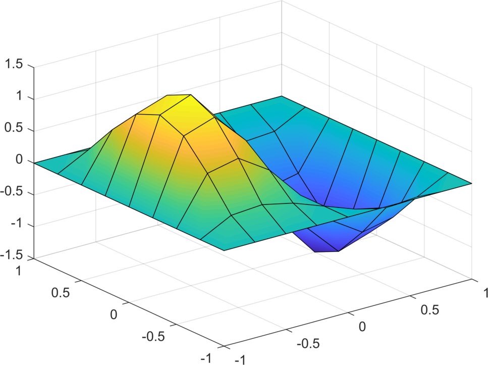
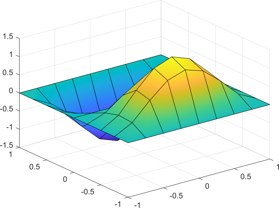
5.3. Implementation details
Our Matlab implementation is based on former vectorized codes of [4, 26, 39] that allow for a fast assembly of various finite element matrices. The code is available at
https://www.mathworks.com/matlabcentral/fileexchange/72991
for download. It includes an own implementation of the Bogner-Fox-Schmit (BFS) rectangular elements for a uniformly refined rectangular mesh, where all rectangular elements are for simplicity of the same size (in our computations ). The basis functions on each rectangle are based on bicubic polynomials, i.e., tensor products of 4 cubic (Hermite) polynomials. They have 16 degrees of freedom with 4 degrees in each of its 4 corner nodes approximating: a function value, its gradient (two components), and the second mixed derivative. Therefore, the initial function must have all these fields available in our simulations. Figure 4 depicts from (37) represented in terms of BFS elements. We recall that BFS elements were also successfully tested in [27] and their implementation was explained in detail in [35].
Acknowledgments
The research of MF was supported by the Deutsche Forschungsgemeinschaft (DFG, German Research Foundation) under Germany’s Excellence Strategy EXC 2044 -390685587, Mathematics Münster: “Dynamics–Geometry–Structure”. MK and JV acknowledge the support by GAČR project 17-04301S.
References
- [1] R.A. Adams, J.J.F. Fournier, Sobolev Spaces (2nd ed), Elsevier, Amsterdam, 2003.
- [2] L. Ambrosio, Minimizing movements, Rend. Accad. Naz. Sci. XL Mem. Mat. Appl., 19 (1995), 191-–246.
- [3] L. Ambrosio, N. Gigli, and G. Savaré, Gradient Flows in Metric Spaces and in the Space of Probability Measures, Lectures Math. ETH Zürich, Birkhäuser, Basel, 2005.
- [4] I. Anjam, J. Valdman, Fast MATLAB assembly of FEM matrices in 2D and 3D: edge elements, Appl. Math. Comput., 267 (2015), 252–263.
- [5] S.S. Antman, Physically unacceptable viscous stresses, Z. Angew. Math. Phys., 49 (1998), 980–988.
- [6] S.S. Antman, Nonlinear Problems of Elasticity, Springer, New York, 2004.
- [7] J.M. Ball, Convexity conditions and existence theorems in nonlinear elasticity, Arch. Ration. Mech. Anal., 63 (1977), 337–403.
- [8] J.M. Ball, J.C. Currie, P.L. Olver, Null Lagrangians, weak continuity, and variational problems of arbitrary order, J. Funct. Anal., 41 (1981), 135–174.
- [9] R.C. Batra, Thermodynamics of non-simple elastic materials, J. Elasticity, 6 (1976), 451–456.
- [10] I. Bock, On Von Kármán equations for viscoelastic plates, J. Comp. Appl. Math., 63 (1995), 277–282.
- [11] I. Bock, J. Jarušek, Solvability of dynamic contact problems for elastic von Kármán plates, SIAM J. Math. Anal., 41 (2009), 37–45.
- [12] I. Bock, J. Jarušek, M. Šilhavý, On the solutions of a dynamic contact problem for a thermoelastic von Kármán plate, Nonlin. Anal.: Real World Appl., 32 (2016), 111–135.
- [13] F.K. Bogner, R.L. Fox and L.A. Schmit, The generation of inter-element compatible stiffness and mass matrices by the use of interpolation formulas, Proceedings of the Conference on Matrix Methods in Structural Mechanics, (1965), 397–444.
- [14] S.C. Brenner, L.R. Scott, The Mathematical Theory of Finite Element Methods, 3rd ed., Springer, New York, 2008.
- [15] G. Capriz, Continua with latent microstructure, Arch. Ration. Mech. Anal., 90 (1985), 43–56.
- [16] V. Casarino, D. Percivale, A variational model for nonlinear elastic plates, J. Convex Anal., 3 (1996), 221–243.
- [17] P.G. Ciarlet, Mathematical Elasticity, Vol. I: Three-dimensional Elasticity, North-Holland, Amsterdam, 1988.
- [18] P.G. Ciarlet, The Finite Element Method for Elliptic Problems, SIAM, Philadelphia, 2002.
- [19] G. Dal Maso, An introduction to -convergence, Birkhäuser, Boston Basel Berlin 1993.
- [20] E. De Giorgi, A. Marino, M. Tosques, Problems of evolution in metric spaces and maximal decreasing curve, Att. Accad. Naz. Lincei Rend. Cl. Sci. Fis. Mat. Natur., 68 (1980), 180–187.
- [21] J.E. Dunn, J. Serrin, On the thermomechanics of interstitial working, Arch. Ration. Mech. Anal., 88 (1985), 95–133.
- [22] M. Friedrich, M. Kružík, On the passage from nonlinear to linearized viscoelasticity, SIAM J. Math. Anal., 50 (2018), 4426–4456.
- [23] M. Friedrich and M. Kružík, Derivation of von Kármán plate theory in the framework of three-dimensional viscoelasticity, preprint, arXiv 1902.10037.
- [24] G. Friesecke, R.D. James, S. Müller, A theorem on geometric rigidity and the derivation of nonlinear plate theory from three-dimensional elasticity, Comm. Pure Appl. Math., 55 (2002), 1461–1506.
- [25] G. Friesecke, R.D. James, S. Müller, A hierarchy of plate models derived from nonlinear elasticity by Gamma-convergence, Arch. Ration. Mech. Anal., 180 (2006), 183–236.
- [26] P. Harasim, J. Valdman, Verification of functional a posteriori error estimates for an obstacle problem in 2D, Kybernetika, 50 (6) (2014), 978–1002.
- [27] S. Krömer, J. Valdman, Global injectivity in second-gradient nonlinear elasticity and its approximation with penalty terms, Mathematics and Mechanics of Solids, 24 (11) (2018), 3644–3673.
- [28] M. Lecumberry, S. Müller, Stability of slender bodies under compression and validity of the von Kármán theory, Arch. Ration. Mech. Anal., 193 (2009), 255–310.
- [29] H. Le Dret, A. Raoult, The nonlinear membrane model as a variational limit of nonlinear three-dimensional elasticity, J. Math. Pures Appl., 73 (1995), 549–578.
- [30] H. Le Dret, A. Raoult, The membrane shell model in nonlinear elasticity: a variational asymptotic derivation, J. Nonl. Sci., 6 (1996), 59–84.
- [31] A. Mielke, C. Ortner, Y. Şengül, An approach to nonlinear viscoelasticity via metric gradient flows, SIAM J. Math. Anal., 46 (2014), 1317–1347.
- [32] A. Mielke, T. Roubíček, Rate-Independent Systems - Theory and Application, Springer, New York, 2015.
- [33] A. Mielke, T. Roubíček, Rate-independent elastoplasticity at finite strains and its numerical approximation, Math. Models & Methods in Appl. Sci., 26 (2016), 2203–2236.
- [34] C. Ortner, Two Variational Techniques for the Approximation of Curves of Maximal Slope, Technical report NA05/10, Oxford University Computing Laboratory, Oxford, UK, 2005.
- [35] J. Valdman, MATLAB Implementation of C1 finite elements: Bogner-Fox-Schmit rectangle, In: Wyrzykowski R., Dongarra J., Deelman E., Karczewski K. (eds) Parallel Processing and Applied Mathematics. PPAM 2019. LNCS, Springer, 2020. (accepted)
- [36] O. Pantz, On the justification of the nonlinear inextensional plate model, Arch. Ration. Mech. Anal., 167 (2003), 179–209.
- [37] J.Y. Park, J.R. Kang, Uniform decay of solutions for von Karman equations of dynamic viscoelasticity with memory, Acta Appl. Math., (2010) 110, 1461–1474.
- [38] P. Podio-Guidugli, Contact interactions, stress, and material symmetry for nonsimple elastic materials, Theor. Appl. Mech., 28–29 (2002), 261–276.
- [39] T. Rahman, J. Valdman, Fast MATLAB assembly of FEM matrices in 2D and 3D: nodal elements, Appl. Math. Comput., 219 (2013), 7151–7158.
- [40] E. Sandier, S. Serfaty, Gamma-convergence of gradient flows with applications to Ginzburg-Landau, Comm. Pure Appl. Math., 57 (2004), 1627-–1672.
- [41] S. Serfaty, Gamma-convergence of gradient flows on Hilbert and metric spaces and applications, Discrete Contin. Dyn. Syst. Ser. A, 31 (2011), 1427-–1451.
- [42] R.A. Toupin, Elastic materials with couple stresses, Arch. Ration. Mech. Anal., 11 (1962), 385–414.
- [43] R.A. Toupin, Theory of elasticity with couple stress, Arch. Ration. Mech. Anal., 17 (1964), 85–112.
- [44] T. von Kármán, Festigkeitsprobleme im Maschinenbau in Encyclopädie der Mathematischen Wissenschaften, vol. IV/4, Leipzig, 1910, 311–385.