A Fair Comparison Between Spatial Modulation and Antenna Selection in Massive MIMO SystemsThanks: This work has been accepted for presentation in the 23rd International ITG Workshop on Smart Antennas (WSA 2019) in Vienna, Austria. The link to the final version in the Proceedings of WSA will be available later.
Abstract
Both antenna selection and spatial modulation allow for low-complexity MIMO transmitters when the number of RF chains is much lower than the number of transmit antennas. In this manuscript, we present a quantitative performance comparison between these two approaches by taking into account implementational restrictions, such as antenna switching.
We consider a band-limited MIMO system, for which the pulse shape is designed, such that the outband emission satisfies a desired spectral mask. The bit error rate is determined for this system, considering antenna selection and spatial modulation. The results depict that for any array size at the transmit and receive sides, antenna selection outperforms spatial modulation, as long as the power efficiency is smaller than a certain threshold level. By passing this threshold, spatial modulation starts to perform superior. Our investigations show that the threshold takes smaller values, as the number of receive antennas grows large. This indi-cates that spatial modulation is an effective technique for uplink transmission in massive MIMO systems.
I Introduction
Recently, sm (sm) has been proposed for single rf (rf) chain multi-antenna transmission. This technique addresses various limitations in mimo (mimo) systems without significant degradation of the performance [1]. The main drawback of conventional mimo techniques arises from the non-negligible cost-complexity issue which is due to
1. inter-channel interference caused by multiple spatial symbols, 2. requiring strict synchronization among transmitting antennas, and 3. employment of a dedicated rf chain per transmit antenna [2, 3].sm is a novel digital modulation technique in which the indexes of active transmit antennas are used as means to convey additional information leading to higher spectral efficiency. More precisely, the incoming bit stream is mapped into two sub-blocks called the signal constellation diagram and spatial constellation diagram. The first sub-block is used to select a symbol from the signal constellation, e.g., phase shift keying, and the second sub-block specifies the position of the active transmit antenna. In the basic form of sm, only one of the transmit antenna is permitted to be active in each channel use. In addition to the overall complexity reduction, this approach leads to elimination of inter-channel interference. As a result, synchronisation of the transmit antennas is not required in this case.
Antenna selection vs. Spatial Modulation
An alternative approach to mitigate the hardware complexity in mimo settings is as (as) [4, 5]. Due to high implementational cost and complexity of massive mimo setups [6, 7], as has received a great deal of attention in the context of massive mimo systems; see for example [8, 9, 10] and the references therein.
In contrast to sm, as selects the transmit antennas based on the csi (csi). Hence, with a given constellation, the number of information bits transmitted in each channel use via as is less than the one achieved by sm. Despite this degradation, as enjoys several advantages compared to sm, such as
- •
- •
The above discussions bring this question into mind: Given a massive mimo setting with a single rf chain at the transmitter, which approach performs superior, when the time-frequency resources are strictly constrained? In this manuscript, we try to answer this question. Our investigations demonstrate that for any number of transmit and receive antennas, there exists a certain level of power efficiency, before which as outperforms sm. As the energy efficiency passes this threshold, sm starts to perform superior. It is further shown that by increasing the size of the receive antenna array, the threshold power efficiency becomes smaller. This observation indicates that sm is an effective technique for uplink transmission in massive mimo settings.
II System Model
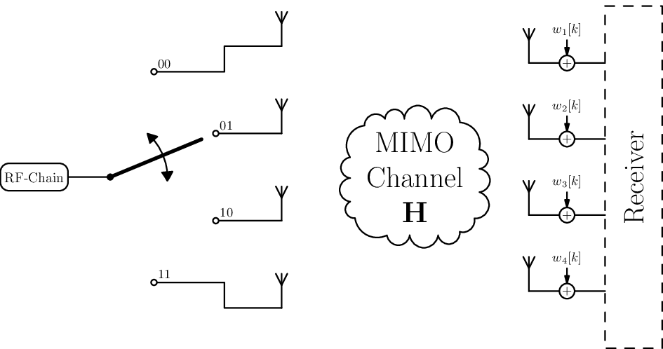
A mimo setting with transmit and receive antennas is considered. The transmitter is equipped with a single rf chain and a switching network which connects the rf chain to a desired transmit antenna at each transmission time interval. This means that at each time interval, only one of the transmit antennas is active. Hence, the receive signal at time interval is given by
| (1) |
In the above equation,
- •
denotes the transmit symbol at time interval drawn from a modulation alphabet .
- •
describes the switching network in time interval . We refer to this vector as the selection vector. It comprises a non-zero entry which corresponds to the active transmit antenna in interval . The selection vector is in general time varying, as the switching network is allowed to switch from one antenna to another, at the beginning of each transmission time interval.
- •
- •
is additive white complex Gaussian noise with zero mean and variance .
We assume that the transmission is performed in tdd (tdd) mode, and hence the channel is reciprocal. The csi is further assumed to be perfectly known at both ends.
II-A Transmission via AS
Under as, the transmit antenna is chosen via a selection algorithm which optimizes a desired performance metric, e.g. the average snr (snr) at the receive side, the achievable rate, or error rate. In the sequel, we consider a conventional selection algorithm. To illustrate the algorithm, let us write the channel matrix as
| (2) |
where for denotes the vector of channel gains between -th transmit antenna and the receive antenna array. The as at the transmit side is performed via the following algorithm:
Algorithm 1:
The transmitter selects the antenna whose corresponding channel gain is maximum. This means that transmit antenna is selected for which we have
It is worth to note that the snr at the receive side is linearly proportional to the channel gain of the transmit antenna. This means that the antenna selected by Algorithm 1 maximizes the receive snr. Since the selection is only based on csi, which is known at the receive side, the receiver can infer , as well.
The selection vector is constructed in this case by setting entry to and all other entries zero. Noting that is a stationary process and is almost constant over a coherence interval, is updated only once per coherence interval when the transmitter employs as. To reflect this, the dependence of on the transmission interval, i.e. argument , is dropped in the sequel under as.
II-B Transmission via SM
sm makes use of the fact that the choice of a particular antenna out of the set of available transmit antennas can also convey information when the index of the transmit antenna is selected via the information bits. To illustrate the idea further, let us assume that the number of transmit antennas is a power of two. In this case, the indices of the transmit antennas, i.e., , is represented via bits. As a result, at each transmission interval, extra bits of information, in addition to , are transmitted when we select the index of the active transmit antenna via the data sequence. Fig. 1 shows an example of sm with four transmit antennas. Here, the first transmit antenna is selected in transmission interval , when the first two bits of data sequence, transmitted in this interval, are . In this particular example, extra information of bits is transmitted in each interval by index modulation, compared to the case with as.
In sm, the selection vector is chosen by the data bits, which vary from one transmission interval to another. This means that, in contrast to as, in this case varies with respect to , and is not known at the receive side. The ml detection, hence, requires to recover both and . As a result, the detection algorithm in this case reads
| (4) |
where is the set of all vectors with a single entry and entries .
II-C Pulse Shaping for SM
As pointed out in [11], switching antennas in each transmission interval distorts pulse shapes if the impulse response of the pulse shaping filter exceeds a symbol duration. To prevent excessive bandwidth occupation, the standard rrc (rrc) filter impulse response is truncated to some acceptable duration. The symbol rate is then reduced such that the pulses are separated in time in order to prevent intersymbol interference. [11] suggests that an acceptable spectral shape is obtained by a rate reduction of factor . The suggested approach deteriorates the effective spectral efficiency.
To design a pulse shape for sm, we note that a square-root Nyquist pulse is not necessary if the symbols do not overlap in time-domain. We hence propose using standard fir (fir) low-pass filters, which are inherently time-limited. Literature knows many distinct fir filter design methods with different optimisation goals, such as linear-phase or minimum-order given a spectral mask with transition zones. However, in a matched filter receiver the actual transfer function form of the pulse shaping filter is irrelevant as long as out-of-band emissions are suppressed to a certain level. On the other hand, all energy which is transmitted out of band is inherently wasted even if a required minimum stopband attenuation is reached. Hence, the non-Nyquist pulse shaping filter should maximise the ratio of energy inside the intended band (passband) and the total energy of its transfer function. This criterion is fulfilled by the Slepian window which maximally concentrates the energy in the main lobe for a given window length [12]. The free design parameter defines the width of the main lobe, whereas increasing the filter length reduces the side lobe level.
To compare the Slepian window with the truncated rrc filter, we set the following requirements:
- 1.
Pulse shaping is accomplished in digital domain.
- 2.
The sampling rate is fixed for both pulse shaping filters to some . For the rrc filter, filter parameter is set to11 1 Note that . . Conventionally, this setting describes a system with symbol rate and fourfold oversampling for pulse shaping.
- 3.
A common roll-off factor is set.
- 4.
To limit emissions outside the bandwidth, a spectral mask is considered allowing a sidelobe level less than dB.
Fig. 2 shows a Slepian window of length and as well as an rrc filter of length samples. As the figure depicts, both filters fulfill the spectral mask. The spectral efficiency is reduced by and , if time-separated pulses of Slepian window and rrc shape are transmitted instead of square-root Nyquist pulses. This indicates that the loss of spectral efficiency, introduced by the Slepian window, is almost four times smaller than the loss imposed by the truncated rrc filter. We hence consider only Slepian pulse shaping in the remainder of this manuscript.
III Performance Comparison
Using sm for band-limited transmission, there exists a clear trade-off which indicates:
- •
On the one hand, sm increases spectral efficiency by exploiting the information conveyed in the index of the selected antenna.
- •
Considering both approaches, a fair comparison of the performance requires the band-limitation constraint to be taken into account. In this respect, we investigate the performance of as and sm in terms of the average bit error rate when the same number of information bits are transmitted per coherence time. Our investigations show that for a fixed number of transmit antennas, sm outperforms as in low and moderate snrs, when the number of receive antennas is relatively large. This observation suggests that in massive mimo settings with reduced hardware complexity, sm is an effective low-complexity scheme for uplink transmission.
III-A Scenario 1: QPSK Transmission for AS and SM
Fig. 3 depicts the average bit error rates, achieved under as and sm, in terms of power efficiency. For both approaches, the modulation scheme is set to qpsk (qpsk). This means that . The power efficiency is quantified in terms of which is defined as the snr divided by the number of bits transmitted in each channel use.
Considering the Slepian window of length , illustrated in Fig. 2, the symbol rate in sm transmission is downscaled by factor . To approximately compensate the reduced symbol rate, the number of transmit antennas is set for both approaches to
| (5) |
where denotes rounding to the nearest integer and bit per channel use is the spectral efficiency of qpsk. In this case, the total spectral efficiencies for as and sm considering a roll-off factor of and QPSK modulation read
| (6a) | ||||
| (6b) | ||||
To investigate the impact of receive array size, the number of receive antennas is swept over . As Fig.3 shows, for all choices of , the as approach initially performs superior to sm. However, as the snr grows, the curves for as and sm meet at some point from where sm starts to outperform as22 2 For small values of , this crossover point occurs at high snrs, and hence is not seen in the figure.. As grows, this crossover point moves to lower snrs, e.g. for , the point occurs around dB.
The above observation is illustrated considering the following aspects:
- •
- •
- •
Aspect C: With a fixed budget of energy for each channel use, the transmit symbol has higher energy under sm, compared to the case with as. In fact, in sm, bits of information is encoded in the modulation index. These bits do not require energy allocation. Under as, on the other hand, all information bits are transmitted by modulation over the active antenna, and hence the total energy is shared among all the transmitted bits.
At very low values of , Aspects A and B dominate the performance, and hence as outperform sm. As increases, Aspect C starts to be the dominate aspect, and sm becomes superior. Moreover, for a given , the growth in the number of receive antennas makes the impacts of Aspects A and B insignificant. Hence, as increases, sm outperforms as over a larger scope of snrs. This implies that in massive mimo setups, sm is an efficient technique for uplink transmission.
III-B Scenario 2: 8QAM Transmission for AS and QPSK for SM
The investigations on Scenario 1 is extended to the case with 8qam constellation for as in Fig. 4. For sm, the conventional modulation, i.e. qpsk remains unchanged. Instead, the number of bits comprised by the indexing is increased to allow for optimum performance of sm. The spectral efficiency of 8qam is bits per channel use. Hence, the loss in spectral efficiency, due to the reduction in symbol rate, weights more severe for sm. Similar to Scenario 1, we compensate this loss by setting the number of transmit antennas
| (7) |
As a result, the total spectral efficiencies for the both approaches are given by
| (8a) | ||||
| (8b) | ||||
Fig. 4 depicts similar behaviour as in Scenario 1. In this scenario, however, the crossover point occurs at lower snrs compared to qpsk transmission, the gap between the two approaches is larger. This follows from the fact that Aspect C, stated in previous scenario, becomes more significant as the size of transmit constellation set increases. On the other hand, for a low number of receive antennas, Aspect B gets more dominant as a larger support has to be recovered by a the same small number of observations.
III-C Influence of Finite Switching Time
In the above scenarios the switching time between the antennas was assumed to be negligible small. This assumption may not hold for practical systems and switching time needs to be considered [13]. However, finite switching time influences as and sm and in different ways. In as, switching takes place only once during a coherence interval, whereas in sm switching occurs with some probability after each symbol, depending on the data sequence [13]. In order to assure a deterministic (i.e. constant) symbol rate in sm, the switching time must be assumed to be a fixed part of the symbol duration. For completeness sake, it should also be mentioned that a non-negligible fraction of the coherence interval needs to be spent for channel estimation. Since for as and sm full knowledge of csi is assumed, we expect that this fraction is same in both cases and set it to zero for simplicity. Then, the spectral efficiencies of as and sm for a common conventional modulation with spectral efficiency are:
| (9a) | ||||
| (9b) | ||||
Note that in general is much smaller than such that is little influenced by the switching time. In contrast, is essentially inversely proportional to . For example, if sm shall achieve a comparable spectral efficiency as a conventional modulation of rate MSymb/s at some fixed and , needs to be significantly smaller than ns.
IV Conclusion
It has been shown that a Slepian window is well suited as a pulse shaping filter for band-limited sm, where standard square root Nyquist pulses cannot be used. As compared to a truncated rrc filter, the shorter length of the Slepian window at a given maximum sidelobe level allows for a significantly higher symbol rate.
Using the Slepian window sm, our comparison of as and sm under the constraint of equal band-limitation shows that sm performs superior to as for large receive arrays while as outperforms sm for receivers with a low number of antennas. For high data rates, sm requires a large number of transmit antennas to achieve comparable spectral efficiency as in as, which eventually may lead to infeasible antenna array sizes. Contrary to as, spectral efficiency of sm is strongly affected by finite antenna switching time, so that the switching time ultimately sets an upper limit on the symbol rate in sm. Therefore, sm appears to be mostly suited for uplink scenarios in which moderate data rates are required.
V Acknowledgment
The authors would like to thank Nikita Shanin for interesting discussions and his helpful comments on the work.
References
- [1] E. Basar, “Index modulation techniques for 5G wireless networks,” IEEE Communications Magazine, vol. 54, no. 7, pp. 168–175, 2016.
- [2] R. Mesleh, H. Haas, S. Sinanovic, C. W. Ahn, and S. Yun, “Spatial modulation,” IEEE Transactions on Vehicular Technology, vol. 57, no. 4, p. 2228, 2008.
- [3] J. Jeganathan, A. Ghrayeb, L. Szczecinski, and A. Ceron, “Space shift keying modulation for MIMO channels,” IEEE Transactions on Wireless Communications, vol. 8, no. 7, pp. 3692–3703, 2009.
- [4] A. F. Molisch, “MIMO systems with antenna selection-an overview,” in Radio and Wireless Conference, 2003. RAWCON’03. Proceedings. IEEE, 2003, pp. 167–170.
- [5] A. F. Molisch, M. Z. Win, Y.-S. Choi, and J. H. Winters, “Capacity of mimo systems with antenna selection,” IEEE Transactions on Wireless Communications, vol. 4, no. 4, pp. 1759–1772, 2005.
- [6] E. G. Larsson, O. Edfors, F. Tufvesson, and T. L. Marzetta, “Massive MIMO for next generation wireless systems,” IEEE communications magazine, vol. 52, no. 2, pp. 186–195, 2014.
- [7] J. Hoydis, S. Ten Brink, and M. Debbah, “Massive MIMO in the UL/DL of cellular networks: How many antennas do we need?” IEEE Journal on selected Areas in Communications, vol. 31, no. 2, pp. 160–171, 2013.
- [8] A. Bereyhi, S. Asaad, and R. R. Mueller, “Stepwise transmit antenna selection in downlink massive multiuser MIMO,” in WSA 2018; 22nd International ITG Workshop on Smart Antennas. VDE, 2018, pp. 1–8.
- [9] S. Asaad, A. M. Rabiei, and R. R. Müller, “Massive MIMO with antenna selection: Fundamental limits and applications,” IEEE Transactions on Wireless Communications, vol. 17, no. 12, pp. 8502–8516, 2018.
- [10] H. Li, L. Song, and M. Debbah, “Energy efficiency of large-scale multiple antenna systems with transmit antenna selection,” IEEE Transactions on Communications, vol. 62, no. 2, pp. 638–647, 2014.
- [11] K. Ishibashi and S. Sugiura, “Effects of antenna switching on band-limited spatial modulation,” IEEE Wireless Communications Letters, vol. 3, no. 4, pp. 345–348, 2014.
- [12] D. Slepian, “Prolate spheroidal wave functions, fourier analysis, and uncertainty — v: the discrete case,” The Bell System Technical Journal, vol. 57, no. 5, pp. 1371–1430, May 1978.
- [13] E. Soujeri and G. Kaddoum, “The impact of antenna switching time on spatial modulation,” IEEE Wireless Communications Letters, vol. 5, no. 3, pp. 256–259, June 2016.
- MIMO
- multiple-input multiple-output
- CSI
- channel state information
- TDD
- time division duplexing
- AWGN
- Additive White Gaussian Noise
- i.i.d.
- independent and identically distributed
- SM
- spatial modulation
- BS
- Base Station
- AS
- antenna selection
- LSE
- Least Squared Error
- r.h.s.
- right hand side
- l.h.s.
- left hand side
- w.r.t.
- with respect to
- RS
- Replica Symmetry
- RSB
- Replica Symmetry Breaking
- PAPR
- Peak-to-Average Power Ratio
- RZF
- Regularized Zero Forcing
- SNR
- Signal-to-Noise Ratio
- RF
- radio frequency
- ML
- maximum likelihood
- RRC
- root-raise-cosine
- BPSK
- binary phase shift keying
- QPSK
- quadrature phase shift keying
- 8QAM
- eight point quadrature amplitude modulation
- FIR
- finite impulse response