跳到论文正文
W Papers独立论文阅读器 arXiv:1904.01864 论文正文 计算阅读时间 · 0%
引用这篇论文根据当前论文元数据生成,正式投稿前建议核对。


License: arXiv.org perpetual non-exclusive license
arXiv:1904.01864v2 [eess.SP] 13 Nov 2020

Online Topology Identification from Vector Autoregressive Time Series Thanks: The work in this paper was supported by the SFI Offshore Mechatronics grant 237896/E30, the PETROMAKS Smart-Rig grant 244205 and the IKTPLUSS Indurb grant 270730/O70 from the Research Council of Norway. Thanks: The authors are with the WISENET Lab, Dept. of ICT, University of Agder, Jon Lilletunsvei 3, Grimstad, 4879 Norway. E-mails:{bakht.zaman, luismiguel.lopez, daniel.romero, baltasar.beferull}@uia.no.Thanks: The material in this work was presented, in part, at CAMSAP 2017 [1].

Bakht Zaman    Luis Miguel Lopez Ramos    Affiliation: Daniel Romero,  and Baltasar Beferull-Lozano, 
Abstract

Causality graphs are routinely estimated in social sciences, natural sciences, and engineering due to their capacity to efficiently represent the spatiotemporal structure of multi-variate data sets in a format amenable for human interpretation, forecasting, and anomaly detection. A popular approach to mathematically formalize causality is based on vector autoregressive (VAR) models and constitutes an alternative to the well-known, yet usually intractable, Granger causality. Relying on such a VAR causality notion, this paper develops two algorithms with complementary benefits to track time-varying causality graphs in an online fashion. Their constant complexity per update also renders these algorithms appealing for big-data scenarios. Despite using data sequentially, both algorithms are shown to asymptotically attain the same average performance as a batch estimator which uses the entire data set at once. To this end, sublinear (static) regret bounds are established. Performance is also characterized in time-varying setups by means of dynamic regret analysis. Numerical results with real and synthetic data further support the merits of the proposed algorithms in static and dynamic scenarios.

I Introduction

Inferring causal relations among time series finds countless applications in social sciences, natural sciences, and engineering. These relations are typically encoded as the edges of a causality graph, where each node corresponds to a time series, and oftentimes reveal the topology of e.g. an underlying social, biological, or brain network [2]. Causality graphs may also offer valuable insights into the spatio-temporal structure of time series and assist data processing tasks such as forecasting [3], signal reconstruction [4], anomaly detection [5], and dimensionality reduction [6]. In some applications, graphs capturing different forms of causality can be constructed based on domain knowledge; see e.g. [7, Ch. 8]. However, this approach is often impractical in the aforementioned applications due to the large dimension of the data or because such prior knowledge is unavailable. Instead, causality graphs need to be inferred from data in these situations. This paper accomplishes this task in an online fashion.

Identifying graphs capturing the spatiotemporal “interactions” among time series has attracted great attention [2, 8]. Some approaches focus on instantaneous interactions, i.e., they disregard the temporal structure. The simplest one is to connect two nodes if the sample correlation between the associated time series exceeds a certain threshold [2]. To distinguish mediated from unmediated interactions [2, Sec. 7.3.2], one may resort to conditional independence, partial correlations, Markov random fields, or other approaches in graph signal processing; see e.g. [9, 10, 11, 7, 12, 13]. For directed interactions, one may employ structural equation models (SEM) [14] (see also [15] and references therein) or Bayesian networks [7, Sec. 8.1]. However, these methods account only for memoryless interactions, i.e., they cannot accommodate delayed interactions where the value of a time series at a given time instant is related to the past values of other time series.

The earliest effort to formalize the notion of causality among time series is due to Granger [16] and relies on the rationale that the cause precedes the effect. A time series is said to be Granger-caused by another if the optimal prediction error of the former is decreased when the past of the latter is taken into account. Albeit elegant, this definition is generally impractical since the optimal prediction error is difficult to determine [17, p. 33], [18]. Thus, alternative causality definitions based on vector autoregressive (VAR) models are typically preferred [19, 20, 21]. VAR causality is determined from the support of VAR matrix parameters and is equivalent to Granger causality [22, Chap. 2] in certain cases (yet sometimes treated as equivalent [20, 21]). VAR causality is further motivated by the widespread usage of VAR models to approximate the response of systems of linear partial differential equations [23] and, more generally, in disciplines such as econometrics, bio-informatics, neuroscience, and engineering [24, 25, 26]. VAR topologies are estimated assuming Gaussianity and stationarity in [27, 28] and assuming sparsity in [29, 30, 31, 32]. All these approaches assume that the graph does not change over time. Since this is not the case in many applications, approaches have been devised to identify undirected time-varying topologies [33, 34] and directed piecewise-constant time-varying topologies [35].

The complexity of all previously discussed approaches becomes prohibitive for long observation windows since they process the entire data set at once and cannot accommodate data arriving sequentially. The modern approach to tackle these issues is online optimization, where an estimate is refined with every new data instance. Existing online topology identification algorithms include [36, 15],[37, 38, 39], and [40], but they only account for memoryless interactions.

The present work is the first to propose online algorithms to estimate the memory-aware causality graphs associated with a collection of time series11 1 The related work in [41] was run in parallel and published after the conference version [1] of this work.. We take as a starting point an online algorithm for estimating directed VAR causality graphs which basically minimizes a sequential, sparse topology identification criterion by means of a composite-objective iteration [42]. This procedure, which we termed TISO (Topology Identification via Sparse Online learning) throughout the paper, promotes sparse updates and enjoys constant computational complexity and memory requirements per iteration, which renders it suitable for sequential and big-data scenarios. Building upon this basic algorithm, the contributions of the present paper include the derivation of a more advanced algorithm, theoretical results that characterize the performance of both algorithms, and empirical validation of their performance through extensive experiments with synthetic and real data sets.

The proposed algorithm is named Topology Identification via Recursive Sparse Online learning (TIRSO), which substantially improves the tracking performance of TISO and robustness to input variability by minimizing a novel estimation criterion inspired by recursive least squares (RLS) where the instantaneous loss function accounts for past samples. TIRSO inherits certain benefits of TISO but incurs a moderate increase in computational complexity, which is still constant per iteration.

We summarize our theoretical results, which constitute the main contribution of our paper: (R1) it is established that the hindsight solution of TISO and TIRSO are asymptotically the same; (R2) The performance of TISO and TIRSO is analyzed in terms of static regret bounds, which are sublinear and suggest that TIRSO outperforms TISO. Hence, in the long run, these algorithms perform as well as the best (batch) predictor in hindsight, which supports their adoption for online topology identification. The static regret analysis goes beyond simply stating that the regret is sublinear (which is a direct consequence of applying the algorithm in [42] to the aforementioned criterion), but rather establishes a bound based on properties of the time series that can be checked in practice; (R3) A logarithmic regret bound is proved for TIRSO (such a bound has been proven for TIRSO and could not be proven for TISO thanks to the strong convexity of the loss function). (R4) To analyze the performance of TIRSO when the topology is time-varying, a dynamic regret bound is derived. Moreover, the steady-state error of TIRSO in time-varying scenarios is quantified in terms of the data properties. Remarkably, the performance (regret) analysis does not require probabilistic assumptions, which endows the developed approaches with high generality.

The conference version [1] of this work presents two online algorithms that are different from the algorithms presented here. One is based on the subgradient approximation for regularized RLS proposed in [43] and has computational complexity comparable to that of TIRSO, and the other one is based on a block coordinate minimization via Newton’s method and has lower computational complexity for large networks with small process order. In addition, no convergence guarantees were provided.

The rest of the paper is organized as follows: Sec. II presents the model, a batch estimation criterion, and background on online optimization. Sec. III develops TISO and TIRSO. Sec. IV and Sec. V respectively assess performance analytically and via simulations, whereas Sec. VI concludes the paper. All code will be made public at the authors’ websites.

Notation. Bold lowercase (uppercase) letters denote column vectors (matrices). Operators 𝔼⁡[⋅]\mathbb{E}[\cdot], ∇\nabla, ∇~\tilde{\nabla}, ∂\partial, (⋅)⊤(\cdot)^{\top}, vec⁡(⋅)\mathrm{vec}(\cdot), λmax​(⋅)\lambda_{\mathrm{max}}(\cdot), ℛ⁡(⋅)\mathcal{R}(\cdot), (⋅)†(\cdot)^{\dagger}, and diag⁡(⋅)\mathrm{diag}(\cdot) respectively denote expectation, gradient, subgradient, sub-differential, matrix transpose, vectorization, maximum eigenvalue, range or column space, pseudo-inverse, and diagonal of a matrix. Symbols 𝟎N\bm{0}_{N}, 𝟏N\bm{1}_{N}, 𝟎N×N\bm{0}_{N\times N}, and 𝑰N\bm{I}_{N} respectively represent the all-zero vector of size NN, the all-ones vector of size NN, the all-zero matrix of size N×NN\times N, and the size-NN identity matrix. Also, [⋅]+=max⁡(⋅,0)[\cdot]_{+}=\mathrm{max}(\cdot,0). For functions f⁡(x)f(x) and g⁡(x)g(x), the notation f⁡(x)∝g⁡(x)f(x)\propto g(x) means ∃a>0,b:f⁡(x)=a​g​(x)+b\exists a>0,b:f(x)=ag(x)+b. The operator 𝟙\mathds{1} is the indicator satisfying 𝟙​{x}=1\mathds{1}\{x\}=1 if xx is true and 𝟙​{x}=0\mathds{1}\{x\}=0 otherwise. Finally, for time series, the notation {yn​[t]}t\{y_{n}[t]\}_{t} corresponds to {yn​[t]}t∈ℤ\{y_{n}[t]\}_{t\in\mathbb{Z}}.

II Preliminaries

After outlining the notion of directed causality graphs, this section reviews how these graphs can be identified in a batch fashion. Later, the basics of online optimization are described.

II-A Directed Causality Graphs

Consider a collection of NN time series {yn​[t]}t\{y_{n}[t]\}_{t}, n=1,…,Nn=1,...,N, where yn​[t]y_{n}[t] denotes the value of the nn-th time series at time tt. A causality graph 𝒢≜(𝒱,ℰ)\mathcal{G}\!\triangleq\!(\mathcal{V},\mathcal{E}) is a graph where the nn-th vertex in 𝒱={1,…,N}\mathcal{V}\!=\!\{1,\ldots,N\} is identified with the nn-th time series {yn​[t]}t\{y_{n}[t]\}_{t} and there is an edge (or arc) from n′n^{\prime} to nn (i.e. (n,n′)∈ℰ(n,n^{\prime})\in\mathcal{E}) if and only if (iff) {yn′​[t]}t\{y_{n^{\prime}}[t]\}_{t} causes {yn​[t]}t\{y_{n}[t]\}_{t} according to a certain causality notion. For the reasons outlined in Sec. I, a prominent notion of causality described later in this section can be defined using VAR models. To this end, let 𝒚⁡[t]≜[y1​[t],…,yN​[t]]⊤\bm{y}[t]\!\triangleq\![y_{1}[t],\ldots,y_{N}[t]]^{\top} and define a VAR time series {𝒚⁡[t]}t\{\bm{y}[t]\}_{t} as a sequence generated by the order-PP VAR model[22]

𝒚⁡[t]=∑p=1P𝑨p​𝒚​[t−p]+𝒖⁡[t],\bm{y}[t]=\textstyle{\sum_{p=1}^{P}}\bm{A}_{p}\bm{y}[t-p]+\bm{u}[t], (1)

where 𝑨p∈ℝN×N,p=1,…,P\bm{A}_{p}\!\in\!\mathbb{R}^{N\times N},p=~\!1,\ldots,P, are the VAR parameters22 2 For the sake of clarity, matrices {𝑨p}p=1P\{\bm{A}_{p}\}_{p=1}^{P} are deemed constant throughout this section. However, all the notions explained here can be easy generalized to time-varying scenarios, as detailed in subsequent sections. and 𝒖⁡[t]≜[u1​[t],…,uN​[t]]⊤\bm{u}[t]\!\triangleq\![u_{1}[t],\ldots,u_{N}[t]]^{\top} is the innovation process. This process is generally assumed to be a temporally white, zero-mean stochastic process, i.e., 𝔼⁡[𝒖⁡[t]]=𝟎N\mathbb{E}[\bm{u}[t]]=\bm{0}_{N} and 𝔼⁡[𝒖⁡[t]​𝒖⊤​[τ]]=𝟎N×N\mathbb{E}[\bm{u}[t]\bm{u}^{\top}[\tau]]\!=\!\bm{0}_{N\times N} for t≠τt\!\neq\!\tau. Yet, the present work does not even need to assume that 𝒖⁡[t]\bm{u}[t] is random, which benefits its generality; see the remark at the end of Sec. IV. With an,n′(p)a_{n,n^{\prime}}^{(p)} the n,n′n,n^{\prime}-th entry of 𝑨p\bm{A}_{p}, expression (1) becomes

yn​[t]\displaystyle y_{n}[t] =∑n′=1N∑p=1Pan,n′(p)​yn′​[t−p]+un​[t]\displaystyle=\textstyle{\sum_{n^{\prime}=1}^{N}\sum_{p=1}^{P}}a_{n,n^{\prime}}^{(p)}y_{n^{\prime}}[t-p]+u_{n}[t]
=∑n′∈𝒩⁡(n)∑p=1Pan,n′(p)​yn′​[t−p]+un​[t]\displaystyle=\textstyle{\sum_{n^{\prime}\in\mathcal{N}(n)}\sum_{p=1}^{P}}a_{n,n^{\prime}}^{(p)}y_{n^{\prime}}[t-p]+u_{n}[t] (2)

for n=1,…,Nn=1,\ldots,N, where 𝒩⁡(n)≜{n′:𝒂n,n′≠𝟎P}\mathcal{N}(n)\!\triangleq\!\{n^{\prime}\!:\!\bm{a}_{n,n^{\prime}}\neq\bm{0}_{P}\} and 𝒂n,n′≜[an,n′(1),…,an,n′(P)]⊤\bm{a}_{n,n^{\prime}}\!\triangleq\![a_{n,n^{\prime}}^{(1)},\ldots,a_{n,n^{\prime}}^{({P})}]^{\top}. Recognizing the convolution operation in the right-hand side enables one to express (2) as yn​[t]=∑n′∈𝒩⁡(n)an,n′(t)∗yn′​[t]+un​[t]y_{n}[t]=\textstyle{\sum_{n^{\prime}\in\mathcal{N}(n)}}a_{n,n^{\prime}}^{(t)}\ast y_{n^{\prime}}[t]\!+\!u_{n}[t] in signal processing notation. Thus, in a VAR model, yn​[t]y_{n}[t] equals the sum of noise and the output of |𝒩⁡(n)||\mathcal{N}(n)| linear time-invariant filters where the n,n′n,n^{\prime}-th filter has input {yn′​[t]}t\{y_{n^{\prime}}[t]\}_{t} and coefficients {an,n′(p)}p=1P\{a_{n,n^{\prime}}^{(p)}\}_{p=1}^{P}.

When 𝒖⁡[t]\bm{u}[t] is a zero-mean and temporally white stochastic process, the term y^n​[t]≜∑n′∈𝒩⁡(n)∑p=1Pan,n′(p)​yn′​[t−p]\hat{y}_{n}[t]\!\triangleq\!\sum_{n^{\prime}\in\mathcal{N}(n)}\sum_{p=1}^{P}a_{n,n^{\prime}}^{(p)}y_{n^{\prime}}[t-p] in (2) is the minimum mean square error estimator of yn​[t]y_{n}[t] given the previous values of all time series {yn′​[τ],n′=1,…,N,τ<t}\{y_{n^{\prime}}[\tau],n^{\prime}\!=\!1,...,N,\tau<\!t\}; see e.g. [18, Sec. 12.7]. The set 𝒩⁡(n)\mathcal{N}(n) therefore collects the indices of those time series that participate in this optimal predictor of yn​[t]y_{n}[t] or, alternatively, the information provided by time series {yn′​[τ]}τ<t\{y_{n^{\prime}}[\tau]\}_{\tau<t} with n′∉𝒩⁡(n)n^{\prime}\!\notin\!\mathcal{N}(n) is not informative to predict yn​[t]y_{n}[t]. This motivates the following definition of causality, which embodies the spirit of Granger causality (see Sec. I): {yn′​[t]}t\{y_{n^{\prime}}[t]\}_{t} VAR-causes {yn​[t]}t\{y_{n}[t]\}_{t} whenever n′∈𝒩⁡(n)n^{\prime}\!\in\!\mathcal{N}(n). Equivalently, {yn′​[t]}t\{y_{n^{\prime}}[t]\}_{t} VAR-causes {yn​[t]}t\{y_{n}[t]\}_{t} if 𝒂n,n′≠𝟎P\bm{a}_{n,n^{\prime}}\!\neq\!\bm{0}_{P}. A detailed comparison with Granger causality lies out of scope, yet it is worth mentioning that the main distinction lies in the prediction horizon33 3 Whereas VAR causality just pertains to prediction 1 time instant ahead, Granger causality involves prediction of all future samples yn​[t′],t′≥ty_{n}[t^{\prime}],~t^{\prime}\geq t, given the ones up to a certain time instant {yn′​[τ],n′=1,…,N,τ<t}\{y_{n^{\prime}}[\tau],~n^{\prime}=1,\ldots,N,~\tau<t\}. Therefore VAR causality implies Granger causality, but the converse is false.; see [22, Sec. 2.3.1] for a more detailed comparison. VAR causality relations among the NN time series can be represented using a causality graph where ℰ≜{(n,n′):𝒂n,n′≠𝟎P}\mathcal{E}\triangleq\{(n,n^{\prime})\!:\!\bm{a}_{n,n^{\prime}}\!\neq\!\bm{0}_{P}\}. Clearly, in such a graph, 𝒩⁡(n)\mathcal{N}(n) is the in-neighborhood of node nn. To quantify the strength of these causality relations, a weighted graph can be constructed by assigning e.g. the weight ‖𝒂n,n′‖2\|\bm{a}_{n,n^{\prime}}\|_{2} to the edge (n,n′)(n,n^{\prime}).

Refer to caption
Fig. 1: Tensor 𝒜\mathcal{A} collecting the VAR parameter matrices.

With these definitions, the batch problem of identifying a VAR causality graph reduces to estimating the VAR coefficient matrices {𝑨p}p=1P\{\bm{A}_{p}\}_{p=1}^{P} given PP and the observations {𝒚⁡[t]}t=0T−1\{\bm{y}[t]\}_{t=0}^{T-1}. To simplify notation, form the tensor 𝒜\mathcal{A} by stacking the matrices {𝑨p}p=1P\{\bm{A}_{p}\}_{p=1}^{P} along the third dimension as shown in Fig. 1.

II-B Batch Estimation Criterion for Topology Identification

This section presents an estimation criterion to address the batch problem formulated in Sec. II-A. A natural estimate could be pursued through least-squares by minimizing [22]

ℒ(𝒜)≜1 2​(T−P)∑τ=PT−1∥𝒚[τ]−∑p=1P𝑨p𝒚[τ−p]∥22\displaystyle\mathcal{L}\left(\mathcal{A}\right)\triangleq\frac{1}{\,2(T-P)}\sum_{\tau=P}^{T-1}\Big\lVert\bm{y}[\tau]-\sum_{p=1}^{P}\bm{A}_{p}\,\bm{y}[\tau-p]\Big\lVert_{2}^{2}
=12​(T−P)​∑n=1N∑τ=PT−1[yn​[τ]−∑n′=1N∑p=1Pan,n′(p)​yn′​[τ−p]]2.\displaystyle=\frac{1}{2\,(T-P)}\sum_{n=1}^{N}\sum_{\tau=P}^{T-1}\Big[y_{n}[\tau]-\sum_{n^{\prime}=1}^{N}\sum_{p=1}^{P}a_{n,n^{\prime}}^{(p)}\,y_{n^{\prime}}[\tau-p]\Big]^{2}.

This estimation task becomes underdetermined unless the number N​TNT of available data samples meaningfully exceeds the number of unknowns P​N2PN^{2}, or, equivalently, T≥P​N+PT\geq PN+P. Even more, to obtain a reasonable performance, one requires T≫P​N+PT\gg PN+P which may not be possible in practice, especially if the parameters {𝑨p}p=1P\{\bm{A}_{p}\}_{p=1}^{P} remain constant only for short periods of time. To circumvent this limitation, one may note that most causality relations between two time series will be mediated by one or more time series. This means that the causality graph introduced in Sec. II-A is expected to be sparse, meaning that many of the vectors 𝒂n,n′\bm{a}_{n,n^{\prime}} equal zero. Such a sparsity structure can be promoted by properly regularizing the aforementioned least squares objective. To this end, the following criterion has been proposed in [29]:

arg⁡min𝒜​ℒ​(𝒜)+λ​∑n=1N∑n′=1,n′≠nN‖𝒂n,n′‖2,\displaystyle\textstyle\underset{\mathcal{A}}{\arg\min}~\mathcal{L}\left(\mathcal{A}\right)\!+\!\lambda\sum_{n=1}^{N}\sum_{\begin{subarray}{c}n^{\prime}=1,n^{\prime}\neq n\end{subarray}}^{N}\left\lVert\bm{a}_{n,n^{\prime}}\right\rVert_{2}, (3)

where λ>0\lambda>0 is a regularization parameter that can be adjusted e.g. via cross-validation [7, Ch. 1]. The second term in (3) is conventionally referred to as a group-lasso44 4 Although other norms (such as the sum of infinity norms) can be used to enforce group sparsity, recoverability results associated with this norm are provided in [29]. regularizer and the solution to (3) as a group-lasso estimate [44]. This promotes a group-sparse structure in {𝑨p}p=1P\{\bm{A}_{p}\}_{p=1}^{P} to exploit the information that the number of edges in ℰ\mathcal{E} is typically small. Self-connections (𝒂n,n\bm{a}_{n,n},​ n=1,…,Nn=1,...,N) are excluded from the regularization term so that the inferred causal relations pertain to the component of each time series that cannot be predicted using its own past. This is motivated by the improvement in consistency reported in [29]. The criterion (3) can be further motivated on the grounds of the consistency of group-lasso estimators [45].

Remarkably, (3) separates along nn. To see this, let 𝒂n≜[𝒂n,1⊤,𝒂n,2⊤,…,𝒂n,N⊤]⊤∈ℝN​P\bm{a}_{n}\triangleq[\bm{a}_{n,1}^{\top},\bm{a}_{n,2}^{\top},...,\,\bm{a}_{n,N}^{\top}]^{\top}\!\in\!\mathbb{R}^{NP} and

𝒈⁡[t]≜vec⁡([𝒚⁡[t−1],…,𝒚⁡[t−P]]⊤)∈ℝN​P,\displaystyle\bm{g}[t]\triangleq\mathrm{vec}\big(\left[\bm{y}[t-1],\ldots,\bm{y}[t-P]\right]^{\top}\!\big)\in\mathbb{R}^{NP}, (4)

and express ℒ⁡(𝒜)\mathcal{L}(\mathcal{A}) as ℒ⁡(𝒜)=∑n=1Nℓ(n)​(𝒂n)\mathcal{L}(\mathcal{A})\!=\!{\sum_{n=1}^{N}{\ell}^{(n)}(\bm{a}_{n})}, where ℓ(n)(𝒂n)≜1/(T−P)∑t=PT−1ℓt(n)(𝒂n){\ell}^{(n)}(\bm{a}_{n})\!\triangleq\!{1}/(T-P)\sum_{t=P}^{T-1}\ell_{t}^{(n)}(\bm{a}_{n}) and ℓt(n)​(𝒂n)≜1/2​(yn​[t]−𝒈⊤​[t]​𝒂n)2\ell_{t}^{(n)}(\bm{a}_{n})\!\triangleq\!{1}/{2}(y_{n}[t]-\bm{g}^{\top}[t]\bm{a}_{n})^{2}. Then, (3) becomes {𝒂n∗}n=1N=arg​min{𝐚n}n=1N∑n=1N[ℓ(n)(𝐚n)+λ∑n′=1,n′≠nN‖𝐚n,n′‖2],\{{\bm{a}}_{n}^{*}\}_{n=1}^{N}\!=\!\argmin_{\{\bm{a}_{n}\}_{n=1}^{N}}\!\sum_{n=1}^{N}\![{\ell}^{(n)}(\bm{a}_{n})\!\!+\!\!{\lambda}\!\sum_{\begin{subarray}{c}n^{\prime}=1,n^{\prime}\neq n\end{subarray}}^{N}\!\left\lVert\bm{a}_{n,n^{\prime}}\right\rVert_{2}], with

𝒂n∗=arg⁡min𝒂n​ℓ(n)​(𝒂n)+λ​∑n′=1,n′≠nN‖𝒂n,n′‖2\textstyle{\bm{a}}_{n}^{*}=\underset{\bm{a}_{n}}{\arg\min}~{\ell}^{\left(n\right)}(\bm{a}_{n})+{\lambda}\sum_{\begin{subarray}{c}n^{\prime}=1,n^{\prime}\neq n\end{subarray}}^{N}\left\lVert\bm{a}_{n,n^{\prime}}\right\rVert_{2} (5)

for n=1,…,Nn=1,\ldots,N. Thus, the VAR causality graph can be identified by separately estimating the VAR coefficients, and hence incoming edge weights, for each node.

The batch estimation criterion in (5) requires all data {𝒚⁡[t]}t=0T−1\{\bm{y}[t]\}_{t=0}^{T-1} before an estimate can be obtained and cannot track changes. Furthermore, solving (5) eventually becomes prohibitively complex for sufficiently large TT. To address these challenges, this paper adopts the framework of online optimization, which is reviewed in the following subsection.

Remark: As seen in (3), λ\lambda is the same for all candidate edges (n,n′)(n,n^{\prime}). This can be readily replaced with an edge-dependent regularization parameter λn,n′\lambda_{n,n^{\prime}} without any complexity increase to exploit possibly available prior-information about edges.

II-C Background on Online Optimization

This section reviews the fundamental notions of online optimization from a general perspective, not necessarily applied to the problem of topology identification. To this end, consider the generic unconstrained optimization problem

minimize𝒂⁡1T0​∑t=0T0−1ht​(𝒂),\displaystyle\mathop{\text{minimize}}_{\bm{a}}~\frac{1}{T_{0}}\sum_{t=0}^{T_{0}-1}~h_{t}(\bm{a}), (6)

where ht​(𝒂)h_{t}(\bm{a}) is a convex function, which in many applications depends on the data received at time tt. For example, in least squares ht​(𝒂)=∥𝑿⁡[t]​𝒂−𝒚⁡[t]∥22h_{t}(\bm{a})\!=\!\lVert\bm{X}[t]\bm{a}-\bm{y}[t]\rVert_{2}^{2}, where 𝒚⁡[t]\bm{y}[t] and 𝑿⁡[t]\bm{X}[t] are the data vector and matrix made available at time tt. To solve (6), it is necessary that all {ht​(𝒂)}t=0T0−1\{h_{t}(\bm{a})\}_{t=0}^{T_{0}-1} be available. Approaches that process all data at once are termed batch and, hence, suffer from potentially long waiting times, which generally render them inappropriate for real-time operation. Besides, computational complexity and memory generally grow super-linearly with T0T_{0}, which eventually becomes prohibitive.

Online algorithms alleviate these limitations. Let 𝒂⁡[t+1]\bm{a}[t+1] denote an estimate of the solution to (6) at time tt produced by an online algorithm. Online algorithms compute a new 𝒂⁡[t+1]\bm{a}[t+1] every time a new (𝑿⁡[t],𝒚⁡[t])(\bm{X}[t],\bm{y}[t]) data element (or, more generally, a new ht​(𝒂)h_{t}(\bm{a})) is processed. At every iteration, also known as update, 𝒂⁡[t+1]\bm{a}[t+1] is obtained from 𝒂⁡[t]\bm{a}[t], 𝒚⁡[t]\bm{y}[t], 𝑿⁡[t]\bm{X}[t], and possibly some additional information carried from each update to the next. The memory requirements and number of arithmetic operations per iteration must not grow unbounded for increasing tt. This requirement rules out approaches involving solving (6) as a batch problem per update or carrying all the past data {(𝑿⁡[τ],𝒚⁡[τ])}τ=0t−1\{(\bm{X}[\tau],\bm{y}[\tau])\}_{\tau=0}^{t-1} from the (t−1)(t\!-\!1)-th update to the tt-th update. Thus, online algorithms are especially appealing when data vectors are received sequentially or T0T_{0} is so large that batch solvers are not computationally affordable. Additionally, online algorithms can track changes in the underlying model. When 𝒂\bm{a} represents a probabilistic model parameter that must be estimated, the estimate obtained through an online method is generally capable of tracking variations in 𝒂\bm{a} so long as they do not occur too rapidly.

The most common performance metric to evaluate online algorithms is the regret, which quantifies the cumulative loss incurred by an online algorithm relative to the loss corresponding to the optimal constant solution in hindsight. Formally, the (static) regret55 5 The static regret is known simply as regret in earlier works, e.g. [46], and different types of regret were formalized later, see e.g. [47]. at iteration T0−1T_{0}-1 is given by [46]:

Rs[T0]≜∑t=0T0−1[ht​(𝒂⁡[t])−ht​(𝒂∗​[T0])],\displaystyle\begin{aligned} R{{}_{s}[T_{0}]}\triangleq&\sum_{t=0}^{T_{0}-1}[h_{t}\left(\bm{a}[t]\right)-h_{t}\left(\bm{a}^{\ast}[T_{0}]\right)],\end{aligned} (7)

where 𝒂∗​[T0]≜arg​min𝐚⁡(1/T0)​∑t=0T0−1ht​(𝐚)\bm{a}^{\ast}[T_{0}]\triangleq\argmin_{\bm{a}}~({1}/{T_{0}})\sum_{t=0}^{T_{0}-1}h_{t}(\bm{a}) is the optimal constant hindsight solution, i.e., the batch solution after T0T_{0} data vectors have been processed. Observe that the regret in (7) may be negative since the estimates {𝒂⁡[t]}t\{\bm{a}[t]\}_{t} are allowed to depend on tt and, hence, it may hold that ht​(𝒂⁡[t])≤ht​(𝒂∗​[T0])h_{t}(\bm{a}[t])\leq h_{t}(\bm{a}^{\ast}[T_{0}]) for multiple (potentially all) values of tt. In practice, nevertheless, the regret will typically be positive and increase with T0T_{0}. To be deemed admissible, online algorithms must yield a sublinear regret, i.e., R[T0]s/T0→0R{{}_{s}[T_{0}]}/T_{0}\!\rightarrow\!0 as T0→∞T_{0}\!\rightarrow\!\infty. Thus, online algorithm with sublinear regret perform asymptotically as well as the batch solution on average. It is worth noting that the online learning framework does not involve statistical assumptions on the data, which can even be generated by an “adversary” [48].

In dynamic settings where the parameters of the data generating process vary over time, 𝒂∗​[T0]\bm{a}^{\ast}[T_{0}] may not be a suitable reference since its computation involves potentially very old data, namely {ht}t≪T0\{h_{t}\}_{t\ll T_{0}}, which is informative about old values of the true parameters but not about the new values. In those cases, it is customary to compare against the instantaneous minimizer 𝒂∘​[t]≜arg​min𝐚⁡ht​(𝐚)\bm{a}^{\circ}[t]\!\triangleq\!\argmin_{\bm{a}}h_{t}(\bm{a}) by means of the so-called dynamic regret [47], [49]:

Rd​[T0]≜∑t=0T0−1[ht​(𝒂⁡[t])−ht​(𝒂∘​[t])].\displaystyle\begin{aligned} R_{d}[T_{0}]\triangleq&\sum_{t=0}^{T_{0}-1}[h_{t}\left(\bm{a}[t]\right)-h_{t}\left(\bm{a}^{\circ}[t]\right)].\end{aligned}

More details about the dynamic regret are given in Sec. IV-C.

III Online Topology Identification

This section develops online algorithms for the considered problem of topology identification from time series. To this end, cast (5) for the nn-th node in the form (6) by setting

ht​(𝒂n)=ℓt+P(n)​(𝒂n)+λ​∑n′=1,n′≠nN‖𝒂n,n′‖2,\textstyle h_{t}(\bm{a}_{n})=\ell^{(n)}_{t+P}(\bm{a}_{n})+\lambda\sum_{\begin{subarray}{c}n^{\prime}=1,n^{\prime}\neq n\end{subarray}}^{N}\left\lVert\bm{a}_{n,n^{\prime}}\right\rVert_{2}, (8)

for t=0,…,T−P−1t=0,...,T-P-1. The most immediate approach to solve (6) would be applying online subgradient descent (OSGD), whose updates are given by 𝒂n​[t+1]=𝒂n​[t]−αt​𝐰~n​[t]\bm{a}_{n}[t+1]=\bm{a}_{n}[t]-\alpha_{t}\tilde{\mathbf{w}}_{n}[t] with 𝐰~n​[t]\tilde{\mathbf{w}}_{n}[t] a subgradient of hth_{t} at 𝒂n​[t]\bm{a}_{n}[t] and αt\alpha_{t} the step size at time tt. From (8), 𝐰~n​[t]\tilde{\mathbf{w}}_{n}[t] equals ∇ℓt+P(n)​(𝒂n​[t])\nabla\ell^{(n)}_{t+P}(\bm{a}_{n}[t]) plus λ\lambda times a valid subgradient of the form

∇~𝒂n∑n′=1n′≠nN‖𝒂n,n′‖2≜[∇~𝒂n,1⊤‖𝒂n,1‖2,…,∇~𝒂n,n−1⊤‖𝒂n,n−1‖2,𝟎P,∇~𝒂n,n+1⊤‖𝒂n,n+1‖2,…,∇~𝒂n,N⊤‖𝒂n,N‖2]⊤,\textstyle\hskip-14.22636pt\tilde{\nabla}_{\bm{a}_{n}}\!\!\sum_{\begin{subarray}{c}n^{\prime}=1\\ n^{\prime}\neq n\end{subarray}}^{N}\!\left\lVert\bm{a}_{n,n^{\prime}}\right\rVert_{2}\!\triangleq\![\tilde{\nabla}_{\bm{a}_{n,1}}^{\top}\!\left\lVert\bm{a}_{n,1}\right\rVert_{2},\ldots,\tilde{\nabla}_{\bm{a}_{n,n-1}}^{\top}\!\left\lVert\bm{a}_{n,n-1}\right\rVert_{2},\\ \bm{0}_{P},\tilde{\nabla}_{\bm{a}_{n,n+1}}^{\top}\left\lVert\bm{a}_{n,n+1}\right\rVert_{2},\ldots,\tilde{\nabla}_{\bm{a}_{n,N}}^{\top}\left\lVert\bm{a}_{n,N}\right\rVert_{2}]^{\top},

evaluated at 𝒂n​[t]\bm{a}_{n}[t]. For example, for 𝒙∈ℝP\bm{x}\in\mathbb{R}^{P}, set ∇~𝒙​∥𝒙∥2=𝒙/∥𝒙∥2\tilde{\nabla}_{\bm{x}}\lVert\bm{x}\rVert_{2}\!=\!\bm{x}/\lVert\bm{x}\rVert_{2} for 𝒙≠𝟎P\bm{x}\!\neq\!\bm{0}_{P} and ∇~𝒙​∥𝒙∥2=𝟎P\tilde{\nabla}_{\bm{x}}\lVert\bm{x}\rVert_{2}\!=\!\bm{0}_{P} for 𝒙=𝟎P\bm{x}=\bm{0}_{P}. It is easy to see that the resulting iterates 𝒂n​[t]\bm{a}_{n}[t] are not necessarily sparse; see also [42]. Since the solution to the batch problem is indeed sparse for a properly selected λ\lambda, alternative approaches are required

To this end, note that OSGD fails to provide sparse iterates because it implicitly linearizes the instantaneous objective ht​(𝒂n)h_{t}(\bm{a}_{n}). Since the regularizer (last term in (8)) is not differentiable, it is not well approximated by a linear function and, as a result, it fails to promote sparsity. To address this issue, composite algorithms decompose ht​(𝒂n)h_{t}(\bm{a}_{n}) as ht​(𝒂n)=ft(n)​(𝒂n)+Ω(n)​(𝒂n)h_{t}(\bm{a}_{n})\!=\!{f_{t}^{(n)}}(\bm{a}_{n})+{{\Omega}^{(n)}}(\bm{a}_{n}), where ft(n)​(𝒂n){f_{t}^{(n)}}(\bm{a}_{n}) is a convex loss function and Ω(n)​(𝒂n){{\Omega}^{(n)}}(\bm{a}_{n}) is a convex regularizer, and linearize only ft(n)​(𝒂n){f_{t}^{(n)}}(\bm{a}_{n}). Algorithms of this family, which include regularized dual averaging (RDA) [50] and composite objective mirror descent (COMID) [42], solve the generic problem

minimize𝒂n​1T0​∑t=0T0−1[ft(n)​(𝒂n)+Ω(n)​(𝒂n)],\underset{\bm{a}_{n}}{\mathop{\text{minimize}}}~\frac{1}{T_{0}}\sum_{t=0}^{T_{0}-1}\big[{f_{t}^{(n)}}(\bm{a}_{n})+{{\Omega}^{(n)}}(\bm{a}_{n})\big], (9)

by linearizing ft(n)​(𝒂n){f_{t}^{(n)}}(\bm{a}_{n}) but not Ω(n)​(𝒂n){\Omega}^{(n)}(\bm{a}_{n}). This work focuses on COMID since, unlike RDA, there exist bounds for its regret for constant step size when the regularizer is not strongly convex. The COMID update is

𝒂n[t+1]=arg⁡min𝒂n[αt∇~ft(n)⊤(𝒂n[t])(𝒂n−𝒂n[t])+Bψ(𝒂n,𝒂n[t])+αtΩ(n)(𝒂n)],\textstyle{\bm{a}_{n}}[t+1]=\underset{\bm{a}_{n}}{\arg\min}\big[{\alpha_{t}}\tilde{\nabla}{f_{t}^{(n)}}^{\top}(\bm{a}_{n}[t])\left(\bm{a}_{n}-\bm{a}_{n}[t]\right)\\ +B_{\psi}\left(\bm{a}_{n},\bm{a}_{n}[t]\right)+{\alpha_{t}{\Omega}^{(n)}}(\bm{a}_{n})\big], (10)

where ∇~​ft(n)​(𝒂n​[t])\tilde{\nabla}{f_{t}^{(n)}}(\bm{a}_{n}[t]) is a subgradient of ft(n){f_{t}^{(n)}} at point 𝒂n​[t]\bm{a}_{n}[t] (that is, ∇~​ft(n)​(𝒂⁡[t])∈∂ft(n)​(𝒂n​[t])\tilde{\nabla}{f_{t}^{(n)}}(\bm{a}[t])\!\in\!\partial f_{t}^{(n)}(\bm{a}_{n}[t])), αt>0\alpha_{t}\!>\!0 is a step size, and Bψ​(𝒘,𝒗)≜ψ⁡(𝒘)−ψ⁡(𝒗)−∇ψ⊤​(𝒗)​(𝒘−𝒗)B_{\psi}(\bm{w},\bm{v})\triangleq\psi(\bm{w})-\psi(\bm{v})-\nabla\psi^{\top}\left(\bm{v}\right)(\bm{w}-\bm{v}) is the so-called Bregman divergence associated with a ζ\zeta-strongly convex and continuously differentiable function ψ\psi. The strong convexity condition means that Bψ​(𝒘,𝒗)≥(ζ/2)​∥𝒘−𝒗∥2B_{\psi}(\bm{w},\bm{v})\geq({\zeta}/{2})\lVert\bm{w}-\bm{v}\rVert^{2}, which motivates using Bψ​(𝒘,𝒗)B_{\psi}(\bm{w},\bm{v}) as a surrogate of a distance between 𝒘\bm{w} and 𝒗\bm{v}. Thus, the Bregman divergence in (10) penalizes updates 𝒂n​[t+1]\bm{a}_{n}[t+1] lying far from the previous one 𝒂n​[t]\bm{a}_{n}[t], which essentially smoothes the sequence of iterates.

Relative to each term in (9), the loss ft(n){f_{t}^{(n)}} in (10) has been linearized but the regularizer Ω(n)​(𝒂n){{\Omega}^{(n)}}(\bm{a}_{n}) has been kept intact. When Ω(n)​(𝒂n){{\Omega}^{(n)}}(\bm{a}_{n}) is a sparsity-promoting regularizer, then the online estimate 𝒂n​[t+1]\bm{a}_{n}[t+1] is therefore expected to be sparse.

In view of these appealing features, the algorithm proposed in Sec. III-A builds upon COMID to address the problem of online causality graph identification from time series.

III-A Topology Identification via Sparse Online optimization

This section proposes topology identification via sparse online optimization (TISO), an online algorithm for the problem in Sec. II-B that provides a causality graph estimate every time a new 𝒚⁡[t]\bm{y}[t] is processed. The key idea of this first algorithm is to refine the previous topology estimate with the information provided by the new data vector by means of a COMID update.

To this end, express hth_{t} in (8) in the form ht​(𝒂n)=ft(n)​(𝒂n)+Ω(n)​(𝒂n)h_{t}(\bm{a}_{n})={f_{t}^{(n)}}(\bm{a}_{n})+{{\Omega}^{(n)}}(\bm{a}_{n}) by setting

ft(n)​(𝒂n)\displaystyle\textstyle{f_{t}^{(n)}}(\bm{a}_{n}) =ℓt+P(n)​(𝒂n),\displaystyle=\ell_{t+P}^{(n)}(\bm{a}_{n}), (11a)
Ω(n)​(𝒂n)\displaystyle{{\Omega}^{(n)}}(\bm{a}_{n}) =λ​∑n′=1,n′≠nN‖𝒂n,n′‖2,\displaystyle=\lambda\textstyle\sum_{\begin{subarray}{c}n^{\prime}=1,n^{\prime}\neq n\end{subarray}}^{N}\left\lVert\bm{a}_{n,n^{\prime}}\right\rVert_{2}, (11b)

for t=0,…,T−P−1.t\!=\!0,...,T-P-1. To choose Bψ​(𝒘,𝒗)B_{\psi}(\bm{w},\bm{v}), note that (10) with ft(n)​(𝒂n){f_{t}^{(n)}}(\bm{a}_{n}) and Ω(n)​(𝒂n){{\Omega}^{(n)}}(\bm{a}_{n}) given by (11) can be solved in closed form when ψ⁡(⋅)=1/2​∥⋅∥22\psi(\cdot)=1/2\lVert\cdot\rVert_{2}^{2}. In that case, Bψ​(𝒘,𝒗)=1/2​∥𝒘−𝒗∥22B_{\psi}(\bm{w},\bm{v})\!=\!1/2\lVert\bm{w}-\bm{v}\rVert_{2}^{2} and 𝒂n​[t+1]\bm{a}_{n}[t+1] can be found via a modified group soft-thresholding operator, as detailed next. With these expressions, the TISO update after processing {𝒚⁡[τ]}τ=0t\{\bm{y}[\tau]\}_{\tau=0}^{t} is

𝒂n​[t+1]\displaystyle\textstyle{\bm{a}}_{n}[t+1] =arg⁡min𝒂nJ(𝒂n)(n)t,\displaystyle=\underset{\bm{a}_{n}}{\arg\min}~J{{}_{t}^{(n)}}(\bm{a}_{n}), (12)

where

Jt(n)(𝒂n)≜𝒗n⊤[t](𝒂n−𝒂n[t])+12​αt‖𝒂n−𝒂n[t]‖22+λ∑n′=1,n′≠nN‖𝒂n,n′‖2J{{}_{t}^{(n)}}(\bm{a}_{n})\triangleq\bm{v}_{n}^{\top}[t](\bm{a}_{n}-\bm{a}_{n}[t])+\frac{1}{2\alpha_{t}}\left\lVert\bm{a}_{n}-\bm{a}_{n}[t]\right\rVert_{2}^{2}\\ +\lambda\textstyle\sum_{\begin{subarray}{c}n^{\prime}=1,n^{\prime}\neq n\end{subarray}}^{N}\left\lVert\bm{a}_{n,n^{\prime}}\right\rVert_{2} (13)

and (using the vector 𝒈⁡[t]\bm{g}[t] defined in (4))

𝒗n​[t]≜∇ℓt(n)​(𝒂n​[t])=𝒈⁡[t]​(𝒈⊤​[t]​𝒂n​[t]−yn​[t]).\vskip-2.84526pt\bm{v}_{n}[t]\triangleq\nabla{\ell}_{t}^{(n)}(\bm{a}_{n}[t])=\bm{g}[t]\,(\bm{g}^{\top}[t]\,\bm{a}_{n}[t]-y_{n}[t]). (14)

To solve (12) in closed form, expand the squared norm in (13) to obtain

J(𝒂n)(n)t\displaystyle J{{}_{t}^{(n)}}(\bm{a}_{n}) ∝‖𝒂n‖222​αt+𝒂n⊤​(𝒗n​[t]−1αt​𝒂n​[t])+λ​∑n′=1n′≠nN‖𝒂n,n′‖2\displaystyle\propto\!\frac{\|\bm{a}_{n}\|_{2}^{2}}{2\alpha_{t}}\!+\!\bm{a}_{n}^{\top}\big(\bm{v}_{n}[t]\!-\!\frac{1}{\alpha_{t}}\bm{a}_{n}[t]\big)\!+\!\lambda\textstyle\sum_{\begin{subarray}{c}n^{\prime}=1\\ n^{\prime}\neq n\end{subarray}}^{N}\left\lVert\bm{a}_{n,n^{\prime}}\right\rVert_{2}
=∑n′=1N[12​αt∥𝒂n,n′∥22+𝒂n,n′⊤(𝒗n,n′[t]−1αt𝒂n,n′[t])\displaystyle=\sum_{n^{\prime}=1}^{N}\Big[\frac{1}{2\alpha_{t}}\|\bm{a}_{n,n^{\prime}}\|_{2}^{2}\!+\!\bm{a}_{n,n^{\prime}}^{\top}\big(\bm{v}_{n,n^{\prime}}[t]\!-\!\frac{1}{\alpha_{t}}\,\bm{a}_{n,n^{\prime}}[t]\big)
+λ‖𝒂n,n′‖2𝟙{n′≠n}],\displaystyle\quad+\lambda\left\lVert\bm{a}_{n,n^{\prime}}\right\rVert_{2}\mathds{1}\{n^{\prime}\neq n\}\Big], (15)

where 𝒗n​[t]≜[𝒗n,1⊤​[t],…,𝒗n,N⊤​[t]]⊤\bm{v}_{n}[t]\triangleq[\,\bm{v}_{n,1}^{\top}[t],...,\bm{v}_{n,N}^{\top}[t]\,]^{\top} and 𝒗n,n′​[t]∈ℝP​∀n′\bm{v}_{n,n^{\prime}}[t]\!\in\!\mathbb{R}^{P}~\forall n^{\prime}. From (15), it can be observed that the updates in (12) can be computed separately for each group n′=1,…,Nn^{\prime}=1,...,N.

For n′≠nn^{\prime}\neq n, the n′n^{\prime}-th subvector of 𝒂n​[t+1]\bm{a}_{n}[t+1] (or n′n^{\prime}-th group) can be expressed in terms of the so-called multidimensional shrinkage-thresholding operator [51] as:

𝒂n,n′​[t+1]=𝒂n,n′f​[t]​[1−αt​λ‖𝒂n,n′f​[t]‖2]+,{\bm{a}}_{n,n^{\prime}}\left[t+1\right]=\bm{a}_{n,n^{\prime}}^{\text{f}}\left[t\right]\left[1-\frac{\alpha_{t}\,\lambda}{\textstyle\left\lVert\bm{a}_{n,n^{\prime}}^{\text{f}}\left[t\right]\right\rVert_{2}}\right]_{+}, (16)

where 𝒂n,n′f​[t]≜𝒂n,n′​[t]−αt​𝒗n,n′​[t]\bm{a}_{n,n^{\prime}}^{\text{f}}\left[t\right]\!\triangleq\!\bm{a}_{n,n^{\prime}}[t]\!-\!\alpha_{t}\bm{v}_{n,n^{\prime}}[t]. Expression (16) is composed of two terms: whereas 𝒂n,n′f​[t]\bm{a}_{n,n^{\prime}}^{\text{f}}[t] is the result of performing a gradient-descent step in a direction that decreases the instantaneous loss ℓt(n)​(𝒂n){\ell}_{t}^{(n)}(\bm{a}_{n}), the second term promotes group sparsity by setting 𝒂n,n′​[t+1]=𝟎P\bm{a}_{n,n^{\prime}}[t+1]\!=\!\bm{0}_{P} for those groups n′n^{\prime} with ∥𝒂n,n′f​[t]∥2≤αt​λ\lVert\bm{a}_{n,n^{\prime}}^{\text{f}}[t]\rVert_{2}\leq\alpha_{t}\,\lambda. Recalling that each vector 𝒂n,n′\bm{a}_{n,n^{\prime}} corresponds to an edge in the estimated causality graph (see Sec. II-A), expression (16) indicates that only the relatively strong edges (i.e. causality relations) survive. In view of such a shrinkage operation, a larger λ\lambda will result in sparser estimates.

On the other hand, when n′=nn^{\prime}\!=\!n, the n′n^{\prime}-th subvector of 𝒂n​[t+1]\bm{a}_{n}[t+1] in (12) is given by:

𝒂n,n′​[t+1]=𝒂n,n′​[t]−αt​𝒗n,n′​[t]=𝒂n,n′f​[t]{\bm{a}}_{n,n^{\prime}}[t+1]=\bm{a}_{n,n^{\prime}}[t]-\alpha_{t}\bm{v}_{n,n^{\prime}}[t]=\bm{a}_{n,n^{\prime}}^{\text{f}}[t] (17)

and, as intended, no sparsity is promoted on self-connections; see Sec. II-B. Combining (16) and (17), the estimate of the n′n^{\prime}-th group at time t+1t+1 is given by:

𝒂n,n′​[t+1]=𝒂n,n′f​[t]​[1−αtλ𝟙{n≠n′}‖𝒂n,n′f​[t]‖2]+.{\bm{a}}_{n,n^{\prime}}[t+1]=\bm{a}_{n,n^{\prime}}^{\text{f}}\left[t\right]\left[1-\frac{\alpha_{t}\lambda~\mathds{1}\{n\neq n^{\prime}\}}{\textstyle\left\lVert\bm{a}_{n,n^{\prime}}^{\text{f}}\left[t\right]\right\rVert_{2}}\right]_{+}. (18)

The performance of TISO depends on the choice of the step-size sequence {αt}t\{\alpha_{t}\}_{t}, as discussed in Sec. IV. The overall TISO algorithm is listed as Procedure 1. It only requires 𝒪⁡(N2​P)\mathcal{O}(N^{2}P) memory entries to store the last PP data vectors and the last estimate. On the other hand, each update requires 𝒪⁡(N2​P)\mathcal{O}(N^{2}P) arithmetic operations, which is in the same order as the number of parameters to be estimated. Thus, TISO can arguably be deemed a low-complexity algorithm.

Procedure 1 Topology Identification via Sparse Online optimization (TISO)

Input: λ,{αt}t,{𝒚⁡[τ]}τ=0P−1\lambda,\{\alpha_{t}\}_{t},\{\bm{y}[\tau]\}_{\tau=0}^{P-1}
Output: {𝒂n​[τ]}n=1N,τ=P+1,…\{{\bm{a}}_{n}[\tau]\}_{n=1}^{N},\tau=P+1,\ldots
Initialization: 𝒂n[P]=𝟎N​P,n=1,…,N{\bm{a}}_{n}[P]=\bm{0}_{NP},n=1,\ldots,N


1: for t=P,P+1,…t=P,P+1,\ldots do
2:   Receive data vector 𝒚⁡[t]\bm{y}[t]
3:   Form 𝒈⁡[t]\bm{g}[t] via (4)
4:   for n=1,2,…,Nn=1,2,\ldots,N do
5:    𝒗n​[t]=(𝒈⊤​[t]​𝒂n​[t]−yn​[t])​𝒈​[t]\bm{v}_{n}[t]=(\bm{g}^{\top}[t]\,{\bm{a}}_{n}[t]-y_{n}[t])\bm{g}[t]
6:    for n′=1,2,…,Nn^{\prime}=1,2,\ldots,N do
7:      𝒂n,n′f​[t]=𝒂n,n′​[t]−αt​𝒗n,n′​[t]\bm{a}_{n,n^{\prime}}^{\text{f}}[t]=\bm{a}_{n,n^{\prime}}[t]-\alpha_{t}\bm{v}_{n,n^{\prime}}[t]
8:      Compute 𝒂n,n′​[t+1]{\bm{a}}_{n,n^{\prime}}[t+1] via (18)    
9:    end for   
10:   end for
11: end for

The next section will build upon TISO to develop an algorithm with increased robustness to input variability.

III-B Topology Identification via Recursive Sparse Online optimization

As seen in Sec. III-A, each update of TISO depends on the data through the instantaneous loss ℓt(n)​(𝒂n​[t])\ell_{t}^{(n)}(\bm{a}_{n}[t]), which quantifies the prediction error of the newly received vector 𝒚⁡[t]\bm{y}[t] when the VAR parameters 𝒜\mathcal{A} are given by the previous estimate 𝒂n​[t]\bm{a}_{n}[t]. Thus, the residual of predicting each data vector is used only in a single TISO update. Although this renders TISO a computationally efficient algorithm for online topology identification, it also increases sensitivity to noise and input variability. To this end, this section pursues an alternative approach at the expense of a moderate increase in computational complexity and memory requirements.

It is clear from (12) that 𝒂n​[t+1]\bm{a}_{n}[t+1] is determined by 𝒂n​[t]\bm{a}_{n}[t] and 𝒗n​[t]\bm{v}_{n}[t]. The latter incorporates the residual only at time tt. The step size αt\alpha_{t} controls how much variability in the input data propagates to the estimates {𝒂n​[t]}t\{\bm{a}_{n}[t]\}_{t}. When a diminishing step-size sequence is adopted, the influence of each new 𝒚⁡[t]\bm{y}[t] on the estimate becomes arbitrarily small, and the variability of the estimates fades away. However, decreasing sequences cannot be utilized when the application at hand demands tracking changes in the coefficients 𝒜\mathcal{A}. In these settings, a constant step size αt=α\alpha_{t}\!=\!\alpha is preferable. In such a scenario, a desire to reduce output variability would therefore force one to adopt a small α\alpha, but this would hinder TISO from tracking changes in the topology.

An approach to reduce output variability without sacrificing tracking capability will be developed next by drawing inspiration from the connections between TISO, the least mean squares (LMS) algorithm, and the recursive least squares (RLS) algorithm [52]. Indeed, observe that TISO generalizes LMS, which is recovered for λ=0\lambda\!=\!0. To speed up convergence and reduce variability in the output of LMS, it is customary to resort to RLS, which accommodates the received data in a more sophisticated fashion, allowing to control the influence of each data vector on future estimates through forgetting factors.

Along these lines, the trick is to replace the instantaneous loss ℓt(n)​(𝒂n)\ell_{t}^{(n)}(\bm{a}_{n}) in (11) with a running average loss. To maintain tracking capabilities, a heavier weight is assigned to recent data using the exponential window customarily adopted by RLS. Specifically, consider setting ft(n)​(𝒂n)=ℓ~t(n)​(𝒂n){f_{t}^{(n)}}(\bm{a}_{n})\!=\!\tilde{\ell}_{t}^{(n)}(\bm{a}_{n}) in (11) with

ℓ~t(n)​(𝒂n)≜μ​∑τ=Ptγt−τ​ℓτ(n)​(𝒂n),\textstyle\tilde{\ell}_{t}^{(n)}(\bm{a}_{n})\triangleq\mu\sum_{\tau=P}^{t}\gamma^{t-\tau}\ell_{\tau}^{(n)}(\bm{a}_{n}), (19)

where γ∈(0,1)\gamma\!\in\!(0,1) is the user-selected forgetting factor and μ=1−γ\mu\!=\!1-\gamma is set to normalize the exponential weighting window, i.e., μ​∑τ=0∞γτ=1\mu\sum_{\tau=0}^{\infty}\gamma^{\tau}\!=\!1.

Having specified a loss function, the next step is to derive the update equation. In a direct application of COMID to solve (9) with ft(n)​(𝒂n)=ℓ~t(n)​(𝒂n){f_{t}^{(n)}}(\bm{a}_{n})\!=\!\tilde{\ell}_{t}^{(n)}(\bm{a}_{n}), each iteration would involve the evaluation of the gradient of the t−P+1t\!-\!P\!+\!1 terms of ℓ~t(n)\tilde{\ell}_{t}^{(n)}. The computational complexity per iteration would grow with tt and, therefore, the resulting updates would not make up a truly online algorithm according to the requirements expressed in Sec. II-C. To remedy this issue, the structure of (19) will be exploited next to develop an algorithm with constant memory and complexity per iteration. To this end, expand and rewrite (19) to obtain

ℓ~t(n)​(𝒂n)=\displaystyle\tilde{\ell}_{t}^{(n)}\!(\bm{a}_{n})\!= μ2​∑τ=Ptγt−τ​(yn2​[τ]+𝒂n⊤​𝒈​[τ]​𝒈⊤​[τ]​𝒂n−2​yn​[τ]​𝒈⊤​[τ]​𝒂n)\displaystyle\frac{\mu}{2}\!\sum_{\tau=P}^{t}\!\gamma^{t-\tau}\big(y_{n}^{2}[\tau]\!+\!\bm{a}_{n}^{\top}\bm{g}[\tau]\bm{g}^{\top}\![\tau]\bm{a}_{n}\!\!-\!2y_{n}[\tau]\bm{g}^{\top}\![\tau]\bm{a}_{n}\big)
=\displaystyle= 12​𝒂n⊤​𝚽​[t]​𝒂n−𝒓n⊤​[t]​𝒂n+μ2​∑τ=Ptγt−τ​yn2​[τ],\displaystyle\frac{1}{2}\bm{a}_{n}^{\top}\bm{\Phi}[t]\bm{a}_{n}\!-\!\bm{r}_{n}^{\top}[t]\bm{a}_{n}\!+\!\frac{\mu}{2}\sum_{\tau=P}^{t}\gamma^{t-\tau}y_{n}^{2}[\tau], (20)

where

𝚽⁡[t]≜μ​∑τ=Ptγt−τ​𝒈​[τ]​𝒈⊤​[τ],\textstyle\bm{\Phi}[t]\triangleq\mu\sum_{\tau=P}^{t}\,\gamma^{t-\tau}\bm{g}[\tau]\,\bm{g}^{\top}[\tau], (21a)
𝒓n​[t]≜μ​∑τ=Ptγt−τ​yn​[τ]​𝒈​[τ].\textstyle\bm{r}_{n}[t]\triangleq\mu\sum_{\tau=P}^{t}\,\gamma^{t-\tau}y_{n}[\tau]\,\bm{g}[\tau]. (21b)

The variables 𝚽⁡[t]\bm{\Phi}[t] and 𝒓n​[t]\bm{r}_{n}[t] can be respectively thought of as a weighted sample autocorrelation matrix and a weighted sample cross-correlation vector. The key observation here is that, as occurs in RLS, these quantities can be updated recursively as 𝚽⁡[t]=γ​𝚽​[t−1]+μ​𝒈​[t]​𝒈⊤​[t]\bm{\Phi}[t]=\gamma\,\bm{\Phi}[t-1]+\mu\,\bm{g}[t]\,\bm{g}^{\top}[t] and 𝒓n​[t]=γ​𝒓n​[t−1]+μ​yn​[t]​𝒈​[t]\bm{r}_{n}[t]=\gamma\,\bm{r}_{n}[t-1]+\mu\,y_{n}[t]\,\bm{g}[t]. Noting that

∇ℓ~t(n)​(𝒂n)=𝚽⁡[t]​𝒂n−𝒓n​[t],\nabla\tilde{\ell}_{t}^{(n)}(\bm{a}_{n})=\bm{\Phi}[t]\bm{a}_{n}-\bm{r}_{n}[t], (22)

and letting 𝒗~n​[t]≜[𝒗~n,1⊤​[t],…,𝒗~n,N⊤​[t]]⊤≜∇ℓ~t(n)​(𝒂n​[t]){\tilde{\bm{v}}}_{n}[t]\triangleq[{\tilde{\bm{v}}}_{n,1}^{\top}[t],\ldots,{\tilde{\bm{v}}}_{n,N}^{\top}[t]]^{\top}\!\triangleq\!\nabla\tilde{\ell}_{t}^{(n)}(\bm{a}_{n}[t]), the estimate 𝒂~n​[t+1]{{\tilde{\bm{a}}}}_{n}[t+1] after receiving {𝒚⁡[τ]}τ=0t\{\bm{y}[\tau]\}_{\tau=0}^{t} becomes

𝒂~n​[t+1]\displaystyle\textstyle{{\tilde{\bm{a}}}}_{n}[t+1] =arg⁡min𝒂~nJ~(𝒂~n)(n)t,\displaystyle=\underset{{\tilde{\bm{a}}}_{n}}{\arg\min}~\tilde{J}{{}_{t}^{(n)}}({\tilde{\bm{a}}}_{n}),\vskip-5.69054pt (23)

where

J~t(n)(𝒂~n)≜𝒗~n⊤[t](𝒂~n−𝒂~n[t])+12​αt‖𝒂~n−𝒂~n[t]‖22+λ∑n′=1,n′≠nN‖𝒂~n,n′‖2.\tilde{J}{{}_{t}^{(n)}}({\tilde{\bm{a}}}_{n})\triangleq{\tilde{\bm{v}}}_{n}^{\top}[t]({\tilde{\bm{a}}}_{n}-{\tilde{\bm{a}}}_{n}[t])+\frac{1}{2\alpha_{t}}\left\lVert{\tilde{\bm{a}}}_{n}-{\tilde{\bm{a}}}_{n}[t]\right\rVert_{2}^{2}\\ +\lambda\textstyle\sum_{\begin{subarray}{c}n^{\prime}=1,n^{\prime}\neq n\end{subarray}}^{N}\left\lVert{\tilde{\bm{a}}}_{n,n^{\prime}}\right\rVert_{2}. (24)

Proceeding similarly to Sec. III-A yields the update

𝒂~n,n′​[t+1]=𝒂~n,n′f​[t]​[1−αtλ𝟙{n≠n′}‖𝒂~n,n′f​[t]‖2]+,{{\tilde{\bm{a}}}}_{n,n^{\prime}}[t+1]={\tilde{\bm{a}}}^{\text{f}}_{n,n^{\prime}}[t]\bigg[1-\frac{\alpha_{t}\lambda~\mathds{1}\{n\neq n^{\prime}\}}{\left\lVert{\tilde{\bm{a}}}^{\text{f}}_{n,n^{\prime}}[t]\right\rVert_{2}}\bigg]_{+}, (25)

where 𝒂~n,n′f​[t]≜𝒂~n,n′​[t]−αt​𝒗~n,n′​[t]{\tilde{\bm{a}}}^{\text{f}}_{n,n^{\prime}}[t]\!\triangleq\!{\tilde{\bm{a}}}_{n,n^{\prime}}[t]\!-\!\alpha_{t}{\tilde{\bm{v}}}_{n,n^{\prime}}[t]. Due to the recursive nature of the updates for 𝚽⁡[t]\bm{\Phi}[t] and 𝒓n​[t]\bm{r}_{n}[t], the resulting algorithm is termed Topology Identification via Recursive Sparse Online optimization (TIRSO) and tabulated as Procedure 2.

The choice of the step size affects the convergence properties of TIRSO, as analyzed in Sec. IV. Regarding step size selection, natural choices include (i) constant step size, which is convenient in dynamic setups where changes in the coefficients 𝒜\mathcal{A} need to be tracked over time (see ?THM? ) but also gives rise to performance guarantees in static scenarios (?THM?  and ?THM?  in the supplementary material); (ii) diminishing step size, commonly in the form of 𝒪⁡(1/t)\mathcal{O}(1/\sqrt{t}) or 𝒪⁡(1/t)\mathcal{O}(1/t) (see ?THM? ); or (iii) an adaptive step size that depends on the data, as discussed at the end of Sec. IV-C.

Observe that 𝚽⁡[t]\bm{\Phi}[t] only needs to be updated once per observed sample tt, whereas the vector 𝒓n​[t]\bm{r}_{n}[t] need to be updated for each nn at every tt. The computational complexity is dominated by step 7, which is 𝒪⁡(N3​P2)\mathcal{O}(N^{3}P^{2}) operations per tt. However, exploiting the group-sparse structure of 𝒂~n​[t]{{\tilde{\bm{a}}}}_{n}[t] may reduce the computation by disregarding the columns of 𝚽⁡[t]\bm{\Phi}[t] corresponding to the zero entries of 𝒂~n​[t]{\tilde{\bm{a}}}_{n}[t]. If, for instance, the number of edges is 𝒪⁡(N)\mathcal{O}(N), then the complexity of TIRSO becomes 𝒪⁡(N2​P2)\mathcal{O}(N^{2}P^{2}) per tt. Regarding memory complexity, TIRSO requires N2​P2N^{2}P^{2} memory positions to store 𝚽⁡[t]\bm{\Phi}[t] and N2​PN^{2}P positions to store {𝒓n​[t]}n=1N\{\bm{r}_{n}[t]\}_{n=1}^{N}.

Procedure 2 Topology Identification via Recursive Sparse Online optimization (TIRSO)

Input: γ,μ,P,λ,σ2,{αt}t,{𝒚⁡[τ]}τ=0P−1\gamma,\mu,P,\lambda,\sigma^{2},\{\alpha_{t}\}_{t},\{\bm{y}[\tau]\}_{\tau=0}^{P-1}
Output: {𝒂~n​[t]}n=1N,t=P+1,…\{{{\tilde{\bm{a}}}}_{n}[t]\}_{n=1}^{N},t=P+1,...
Initialization: 𝒂~n[P]=𝟎N​P,n=1,…,N,𝚽[P−1]=σ2𝑰N​P𝒓n[t]=𝟎N​P,n=1,…,N{{\tilde{\bm{a}}}}_{n}[P]=\bm{0}_{NP},n=\!1,...,N,\,\bm{\Phi}[P-1]\!=\!\sigma^{2}\bm{I}_{NP}\\ \bm{r}_{n}[t]=\bm{0}_{NP},n=1,...,N


1: for t=P,P+1,…t=P,P+1,\ldots do
2:   Receive data vector 𝒚⁡[t]\bm{y}[t]
3:   Form 𝒈⁡[t]\bm{g}[t] via (4)
4:   𝚽⁡[t]=γ​𝚽​[t−1]+μ​𝒈​[t]​𝒈⊤​[t]\bm{\Phi}[t]=\gamma\,\bm{\Phi}[t-1]+\mu\,\bm{g}[t]\,\bm{g}^{\top}[t]
5:   for n=1,…,Nn=1,\ldots,N do
6:    𝒓n​[t]=γ​𝒓n​[t−1]+μ​yn​[t]​𝒈​[t]\bm{r}_{n}[t]=\gamma\,\bm{r}_{n}[t-1]+\mu\,y_{n}[t]\,\bm{g}[t]
7:    𝒗~n​[t]=𝚽⁡[t]​𝒂~n​[t]−𝒓n​[t]{\tilde{\bm{v}}}_{n}[t]=\bm{\Phi}[t]\,{{\tilde{\bm{a}}}}_{n}[t]-\bm{r}_{n}[t]
8:    for n′=1,2,…,Nn^{\prime}=1,2,\ldots,N do
9:      𝒂~n,n′f​[t]=𝒂~n,n′​[t]−αt​𝒗~n,n′​[t]{\tilde{\bm{a}}}^{\text{f}}_{n,n^{\prime}}[t]={\tilde{\bm{a}}}_{n,n^{\prime}}[t]-\alpha_{t}{\tilde{\bm{v}}}_{n,n^{\prime}}[t]
10:      Compute 𝒂~n,n′​[t+1]{{\tilde{\bm{a}}}}_{n,n^{\prime}}[t+1] via (25)    
11:    end for   
12:   end for
13: end for

IV Theoretical Results

In this section, the performance of TISO and TIRSO is analyzed. The upcoming results will make use of one or more of the following assumptions:

  1. A1.

    Bounded samples: There exists By>{\color[rgb]{0,0,0}B}_{y}\!>0\! such that |yn​[t]|2≤By​∀n,t|y_{n}[t]|^{2}\leq{\color[rgb]{0,0,0}B}_{y}~\forall\,n,t.

  2. A2.

    Bounded minimum eigenvalue of 𝚽⁡[t]\bm{\Phi}[t]: There exists βℓ~>0\beta_{\tilde{\ell}}~>~0 such that λmin​(𝚽⁡[t])≥βℓ~,∀t≥P\lambda_{\mathrm{min}}(\bm{\Phi}[t])\geq\beta_{\tilde{\ell}},~\forall\,t\geq P.

  3. A3.

    Bounded maximum eigenvalue of 𝚽⁡[t]\bm{\Phi}[t]: There exists L>0L~>~0 such that λmax​(𝚽⁡[t])≤L,∀t≥P\lambda_{\mathrm{max}}(\bm{\Phi}[t])\leq L,~\forall\,t\geq P.

  4. A4.

    Asymptotically invertible sample covariance: There exists TmT_{m} and β\beta such that

    λmin​(1t−P​∑τ=Pt𝒈⁡[τ]​𝒈⊤​[τ])≥β​∀t≥Tm.\textstyle\lambda_{\mathrm{min}}\left(\frac{1}{t-P}\sum_{\tau=P}^{t}\bm{g}[\tau]\,\bm{g}^{\top}[\tau]\right)\geq\beta~~\forall\,t\geq T_{m}. (26)

Note that A1 entails no loss of generality in real-world applications, where data are bounded and thus By{\color[rgb]{0,0,0}B}_{y} necessarily exists. A2 usually holds in practice unless the data is redundant, meaning that some time series can be obtained as a linear combination of the others. In general, the latter will not be the case e.g. if the data {𝒚⁡[t]}t\{\bm{y}[t]\}_{t} adheres to a continuous probability distribution, in which case 𝚽⁡[t]\bm{\Phi}[t] is positive definite for all t≥Pt\geq P with probability 1. A3 will also hold in practice since it can be shown that it is implied by A1. In particular, if A1 holds, then A3 holds with L=P​N​ByL=PN{\color[rgb]{0,0,0}B}_{y}. Similarly, A26 will also generally hold since it is a weaker version of A2.

Next, the asymptotic equivalence of the batch solutions for TISO and TIRSO is established.

IV-A Asymptotic Equivalence between TISO and TIRSO

To complement the arguments given in Sec. III-B to support the decision of setting ft(n)​(𝒂n)=ℓ~t(n)​(𝒂n){f_{t}^{(n)}}(\bm{a}_{n})\!\!=\!\!\tilde{\ell}_{t}^{(n)}(\bm{a}_{n}), which laid the grounds to develop TIRSO, we establish that the batch problems that TISO and TIRSO implicitly solve become asymptotically equivalent as T→∞T\!\rightarrow\!\infty. To this end, let 𝒂n∗​[T]\bm{a}_{n}^{*}[T] denote the hindsight solution for TISO, which is given by

𝒂n∗​[T]=arg⁡min𝒂n​CT​(𝒂n),\displaystyle\bm{a}_{n}^{*}[T]\!=\!\underset{\bm{a}_{n}}{\arg\min}~{\color[rgb]{0,0,0}C}_{T}(\bm{a}_{n}), (27)

where

CT​(𝒂n)≜1T−P​∑t=PT−1[ℓt(n)​(𝒂n)+λ​∑n′=1,n′≠nN‖𝒂n,n′‖2].\displaystyle\textstyle{\color[rgb]{0,0,0}C}_{T}(\bm{a}_{n})\!\triangleq\!\frac{1}{T-P}\!\sum_{t=P}^{T-1}\!\Big[\ell_{t}^{(n)}(\bm{a}_{n})\!+\!\!\lambda\!\sum_{\begin{subarray}{c}n^{\prime}=1,n^{\prime}\neq n\end{subarray}}^{N}\!\left\lVert\bm{a}_{n,n^{\prime}}\right\rVert_{2}\!\Big]. (28)

Observe that (28) is identical to the objective in the batch criterion (5). Likewise, let 𝒂~n∗​[T]{\tilde{\bm{a}}}^{*}_{n}[T] denote the hindsight solution of TIRSO, which is given by

𝒂~n∗​[T]=arg⁡min𝒂n​C~T​(𝒂n)\displaystyle{\tilde{\bm{a}}}^{*}_{n}[T]=\underset{\bm{a}_{n}}{\arg\min}~~{\color[rgb]{0,0,0}\tilde{C}}_{T}(\bm{a}_{n})\vskip-5.69054pt (29)

with

C~T​(𝒂n)≜1T−P​∑t=PT−1[ℓ~t(n)​(𝒂n)+λ​∑n′=1,n′≠nN‖𝒂n,n′‖2].\displaystyle\textstyle{\color[rgb]{0,0,0}\tilde{C}}_{T}(\bm{a}_{n})\!\triangleq\!\!\frac{1}{T-P}\!\sum_{t=P}^{T-1}\!\Big[\tilde{\ell}_{t}^{(n)}(\bm{a}_{n})\!+\!\lambda\!\sum_{\begin{subarray}{c}n^{\prime}=1,n^{\prime}\neq n\end{subarray}}^{N}\!\left\lVert\bm{a}_{n,n^{\prime}}\right\rVert_{2}\!\Big]. (30)

In this case, (30) no longer coincides with the objective in (5). Therefore, one can argue that the TIRSO algorithm is not pursuing the estimates that minimize the batch criterion (5). This idea is dispelled next by establishing the asymptotic equivalence between minimizing C~T​(𝒂n){\color[rgb]{0,0,0}\tilde{C}}_{T}(\bm{a}_{n}) and minimizing CT​(𝒂n){\color[rgb]{0,0,0}C}_{T}(\bm{a}_{n}), since the latter is identical to (5).

Theorem 1.

Under assumption A1:

  1. 1.

    It holds for all 𝒂n\bm{a}_{n} that limT→∞|CT​(𝒂n)−C~T​(𝒂n)|=0.\displaystyle\lim_{T\rightarrow\infty}|{\color[rgb]{0,0,0}C}_{T}(\bm{a}_{n})-{\color[rgb]{0,0,0}\tilde{C}}_{T}(\bm{a}_{n})|=0.

  2. 2.

    It holds that limT→∞|inf𝒂nCT​(𝒂n)−inf𝒂nC~T​(𝒂n)|=0.\displaystyle\lim_{T\rightarrow\infty}\big|\inf_{\bm{a}_{n}}{\color[rgb]{0,0,0}C}_{T}(\bm{a}_{n})-\inf_{\bm{a}_{n}}{\color[rgb]{0,0,0}\tilde{C}}_{T}(\bm{a}_{n})\big|=0.

  3. 3.

    If, additionally, assumption A2 holds, then limT→∞‖𝒂n∗​[T]−𝒂~n∗​[T]‖2=0.\lim_{T\rightarrow\infty}\|\bm{a}_{n}^{*}[T]-{\tilde{\bm{a}}}_{n}^{*}[T]\|_{2}=0.

Proof:

See Appendix A in the supplementary material. ∎?THM?  essentially establishes not only that the TISO and TIRSO hindsight objectives are asymptotically the same but also that their minima and minimizers asymptotically coincide. Since the TISO hindsight objective equals the batch objective (5), it follows that the TIRSO hindsight objective asymptotically approaches the batch objective (5). This observation is very important since the regret analysis from Sec. IV-B will establish that the TISO and TIRSO estimates asymptotically match their hindsight counterparts.

IV-B Static Regret Analysis

This section characterizes the performance of TISO and TIRSO analytically. Specifically, it is shown that the sequences of estimates produced by these algorithms yield a sublinear static regret, which is a basic requirement in online optimization; see Sec. II-C. Broadly speaking, this property means that, on average and asymptotically, the online estimates perform as well as their hindsight counterparts.

A general definition of the regret metric is given in (7). Since the problem at hand is separable across nodes, it is natural to separately quantify the regret for each node. The total regret will be the sum of the regret for all nodes. Applying this idea and shifting the time index to simplify notation, one can replace Rs​[T0]R_{{s}}[T_{0}] in (7) with Rs(n)​[T0+P−1]R_{s}^{(n)}[T_{0}+P-1], function hth_{t} with ht+P(n)h_{t+P}^{(n)}, and T0T_{0} with T−P+1T-P+1 to write the regret of TISO for the nn-th node at time TT as

Rs(n)​[T]≜∑t=PT[ht(n)​(𝒂n​[t])−ht(n)​(𝒂n∗​[T])],R_{s}^{(n)}[T]\triangleq\sum_{t=P}^{T}\big[h_{t}^{(n)}(\bm{a}_{n}[t])-h_{t}^{(n)}(\bm{a}_{n}^{*}[T])\big], (31)

where ht(n)​(⋅)=ℓt(n)​(⋅)+Ω(n)​(⋅)h_{t}^{(n)}(\cdot)={\ell_{t}^{(n)}}(\cdot)+{{\Omega}^{(n)}}(\cdot) and 𝒂n∗​[T]\bm{a}_{n}^{*}[T] is defined in (27). For TIRSO, the regret for the nn-th node is given by

R~s(n)​[T]≜∑t=PT[h~t(n)​(𝒂~n​[t])−h~t(n)​(𝒂~n∗​[T])],\tilde{R}_{s}^{(n)}[T]\triangleq\sum_{t=P}^{T}\big[\tilde{h}_{t}^{(n)}({\tilde{\bm{a}}}_{n}[t])-\tilde{h}_{t}^{(n)}({\tilde{\bm{a}}}_{n}^{*}[T])\big], (32)

where h~t(n)​(⋅)=ℓ~t(n)​(⋅)+Ω(n)​(⋅)\tilde{h}_{t}^{(n)}(\cdot)={\tilde{\ell}_{t}^{(n)}}(\cdot)+{{\Omega}^{(n)}}(\cdot) and 𝒂~n∗​[T]{\tilde{\bm{a}}}_{n}^{*}[T] is defined in (29).

Since constant step size sequences allow tracking time-varying topologies, one could think of seeking a sublinear bound for the regret. However, it is easy to see (cf. (17) and (18) in the case of TISO) that the sequences of estimates in this case are generally noisy, unless the innovation process 𝒖⁡[t]\bm{u}[t] in (1) is 𝟎N\bm{0}_{N}. For this reason, a sublinear regret bound cannot be obtained for a constant αt\alpha_{t}. However, it is possible to establish sublinear regret when the step size is “asymptotically constant,” as described next.

The idea is to run the selected algorithm in time windows of exponentially increasing length with a step size that differs across windows but is constant within each one. Specifically, let the (m+1)(m+1)-th window, m=1,…,Mm=1,\ldots,M, comprise the time indices t0​2m−1<t≤t0​2mt_{0}2^{m-1}<t\leq t_{0}2^{m} for some user-selected t0≥Pt_{0}\geq P. Set αt=α[m]\alpha_{t}=\alpha_{[m]} for those tt satisfying t0​2m−1<t≤t0​2mt_{0}2^{m-1}<t\leq t_{0}2^{m}. The following result proves sublinear regret for TISO.

Theorem 2.

Let {𝐚n​[t]}t=PT\{\bm{a}_{n}[t]\}_{t=P}^{T} be generated by applying TISO (Procedure 1) with step size αt=α[m]=𝒪⁡(1/t0​2m−1)\alpha_{t}=\alpha_{[m]}=\mathcal{O}(1/\sqrt{t_{0}2^{m-1}}) in the window t0​2m−1<t≤t0​2mt_{0}2^{m-1}<t\leq t_{0}2^{m}, m=1,2,…m=1,2,\ldots Then, the regret of TISO under assumptions A1 and A26 is

Rs(n)​[T]=𝒪⁡(P​N​By​B𝒂2​T),R_{s}^{(n)}[T]=\mathcal{O}\left(PN{\color[rgb]{0,0,0}B}_{y}B_{\bm{a}}^{2}\sqrt{T}\right), (33)

where B𝐚=1/β⁡(By​P​N+By2​P​N+β​By)B_{\bm{a}}=1/\beta({\color[rgb]{0,0,0}B}_{y}\sqrt{PN}+\sqrt{{\color[rgb]{0,0,0}B}_{y}^{2}PN+\beta{\color[rgb]{0,0,0}B}_{y}}).

Proof:

See Appendix B in the supplementary material. ∎

Similarly, the regret of TIRSO is characterized as follows:

Theorem 3.

Let {𝐚~n​[t]}t=PT\{{\tilde{\bm{a}}}_{n}[t]\}_{t=P}^{T} be generated by applying TIRSO (Procedure 2) with step size αt=α[m]=𝒪⁡(1/t0​2m−1)\alpha_{t}=\alpha_{[m]}=\mathcal{O}(1/\sqrt{t_{0}2^{m-1}}) in the window t0​2m−1<t≤t0​2mt_{0}2^{m-1}<t\leq t_{0}2^{m}, m=1,2,…m=1,2,\ldots Then, the regret of TIRSO under assumptions A1, A2, and A3, is

Rs(n)​[T]=𝒪⁡(L​B𝒂~2​T),R_{s}^{(n)}[T]=\mathcal{O}\left(LB_{{\tilde{\bm{a}}}}^{2}\sqrt{T}\right), (34)

where B𝐚~≜1/βℓ~​(By​P​N+By2​P​N+βℓ~​By)B_{{\tilde{\bm{a}}}}\triangleq 1/\beta_{\tilde{\ell}}({\color[rgb]{0,0,0}B}_{y}\sqrt{PN}+\sqrt{{\color[rgb]{0,0,0}B}_{y}^{2}PN+\beta_{\tilde{\ell}}{\color[rgb]{0,0,0}B}_{y}}).

Proof:

See Appendix D in the supplementary material. ∎?THM?  has the same form as ?THM?  with the exception of (79), where the constant term multiplying T\sqrt{T} differs from the one in (33). However, it can be readily shown that L≤P​N​ByL\leq PN{\color[rgb]{0,0,0}B}_{y}, which implies that TIRSO also satisfies (33).

To sum up, both TISO and TIRSO behave asymptotically in the same fashion and provide, on average, the same performance as the hindsight solution of TISO, which coincides with the batch solution in (5). The difference between TISO and TIRSO is, therefore, in the non-asymptotic regime, where TIRSO can track changes in the estimated graph more swiftly than TISO. This is at the expense of a slight increase in the number of arithmetic operations and required memory. Note, however, that TIRSO offers an additional degree of freedom through the selection of the forgetting factor γ\gamma. This enables the user to select the desired point in the trade-off between adaptability to changes and low variability in the estimates.

As demonstrated next, tighter regret bounds can be obtained when a diminishing step size sequence is adopted. Such sequences are of special interest when the VAR coefficients do not change over time. Even in this scenario, the application of online algorithms such as TISO or TIRSO is well-motivated when the number or dimension of the data vectors is prohibitively large to tackle with a batch algorithm.

Theorem 4.

Under assumptions A1, A2, and A3, let {𝐚~n​[t]}t=PT\{{\tilde{\bm{a}}}_{n}[t]\}_{t=P}^{T} be generated by TIRSO (Procedure 2) with αt=1/(βℓ~​t)\alpha_{t}=1/(\beta_{\tilde{\ell}}t). Then, the static regret of TIRSO satisfies

R~s(n)​[T]≤Gℓ~22​βℓ~​(log⁡(T−P+1)+1)+12​αP−1​B𝒂~2,\tilde{R}_{s}^{(n)}[T]\leq\frac{G_{\tilde{\ell}}^{2}}{2\beta_{\tilde{\ell}}}\left(\mathrm{log}(T-P+1)+1\right)+\frac{1}{2\alpha_{P-1}}B_{{\tilde{\bm{a}}}}^{2}, (35)

where Gℓ~≜(1+κ𝚽)​P​N​ByG_{\tilde{\ell}}\triangleq(1+\kappa_{\bm{\Phi}})\sqrt{PN}{\color[rgb]{0,0,0}B}_{y} with κ𝚽=L/βℓ~\kappa_{\bm{\Phi}}=L/\beta_{\tilde{\ell}} and B𝐚~B_{{\tilde{\bm{a}}}} is defined in ?THM? .

Proof:

See Appendix F in the supplementary material. ∎Next, we analyze the performance of TIRSO in dynamic environments.

IV-C Dynamic Regret Analysis of TIRSO

In this section, the performance of TIRSO is analyzed in dynamic settings. Specifically, a dynamic regret bound is derived for TIRSO, and its steady-state tracking error in dynamic scenarios is also discussed. To characterize the performance of TIRSO in dynamic setups, the dynamic regret is defined as:

R~d(n)​[T]≜∑t=PT[h~t(n)​(𝒂~n​[t])−h~t(n)​(𝒂~n∘​[t])],\textstyle\tilde{R}_{d}^{(n)}[T]\triangleq\sum_{t=P}^{T}\big[\tilde{h}_{t}^{(n)}({\tilde{\bm{a}}}_{n}[t])-\tilde{h}_{t}^{(n)}({\tilde{\bm{a}}}_{n}^{\circ}[t])\big], (36)

where 𝒂~n​[t]{\tilde{\bm{a}}}_{n}[t] is the TIRSO estimate and 𝒂~n∘​[t]=arg⁡min𝒂~n​h~t(n)​(𝒂~n){\tilde{\bm{a}}}_{n}^{\circ}[t]=\arg\min_{{\tilde{\bm{a}}}_{n}}\tilde{h}_{t}^{(n)}({\tilde{\bm{a}}}_{n}). The dynamic regret in (36) compares the estimate 𝒂~n​[t]{\tilde{\bm{a}}}_{n}[t] with 𝒂~n∘​[t]{\tilde{\bm{a}}}_{n}^{\circ}[t] in terms of the metric h~t(n)​(⋅)\tilde{h}_{t}^{(n)}(\cdot). As opposed to 𝒂~n∘​[t]{\tilde{\bm{a}}}_{n}^{\circ}[t], estimate 𝒂~n​[t]{\tilde{\bm{a}}}_{n}[t] does not “know” h~t(n)​(⋅)\tilde{h}_{t}^{(n)}(\cdot) since 𝒂~n​[t]{\tilde{\bm{a}}}_{n}[t] is obtained from {𝒚⁡[τ]}τ<t\{\bm{y}[\tau]\}_{\tau<t} whereas h~t(n)​(⋅)\tilde{h}_{t}^{(n)}(\cdot) depends on both {𝒚⁡[τ]}τ<t\{\bm{y}[\tau]\}_{\tau<t} and 𝒚⁡[t]\bm{y}[t]. This means that the dynamic regret captures the ability of an algorithm to attain small future residuals. Furthermore, note that comparing with 𝒂~n∘​[t]{\tilde{\bm{a}}}_{n}^{\circ}[t] is highly meaningful in the present case since, by definition, 𝒂~n∘​[t]=arg⁡min𝒂~n​μ​∑τ=Ptγt−τ​ℓτ(n)​(𝒂~n)+λ​∑n′=1,n′≠nN‖𝒂~n,n′‖2{\tilde{\bm{a}}}_{n}^{\circ}[t]=\arg\min_{{\tilde{\bm{a}}}_{n}}\mu\sum_{\tau=P}^{t}\gamma^{t-\tau}\ell_{\tau}^{(n)}({\tilde{\bm{a}}}_{n})+\lambda\textstyle\sum_{\begin{subarray}{c}n^{\prime}=1,n^{\prime}\neq n\end{subarray}}^{N}\left\lVert{\tilde{\bm{a}}}_{n,n^{\prime}}\right\rVert_{2}, which therefore minimizes a version of the batch (5) or hindsight (29) objectives where the more recent residuals are weighted more heavily. Thus, 𝒂~n∘​[t]{\tilde{\bm{a}}}_{n}^{\circ}[t] constitutes a significant estimator in dynamic setups and therefore the dynamic regret also quantifies the ability of an estimator to track changes.

It can be easily shown that the static regret is upper-bounded by the dynamic regret. The dynamic regret in (36) would coincide with the static regret if 𝒂~n∘​[t]{\tilde{\bm{a}}}_{n}^{\circ}[t] were replaced with arg⁡min⁡∑t=PT𝒂~n⁡h~t(n)​(𝒂~n)\arg\min_{{\tilde{\bm{a}}}_{n}}\sum_{t=P}^{T}\tilde{h}_{t}^{(n)}({\tilde{\bm{a}}}_{n}). Attaining a low dynamic regret is therefore more challenging because the estimator under consideration is compared with a time-varying reference. This implies that a sublinear dynamic regret may not be attained if this time-varying reference changes too rapidly, which generally occurs when the tracked parameters vary too quickly. For this reason, the dynamic regret is commonly upper-bounded in terms of the cumulative distance between two consecutive instantaneous optimal solutions, known as path length:

W(n)​[T]≜∑t=P+1T‖𝒂~n∘​[t]−𝒂~n∘​[t−1]‖2.\textstyle W^{(n)}[T]\triangleq\sum_{t=P+1}^{T}\left\lVert{\tilde{\bm{a}}}_{n}^{\circ}[t]-{\tilde{\bm{a}}}_{n}^{\circ}[t-1]\right\rVert_{2}. (37)

Next, we bound the dynamic regret of TIRSO.

Theorem 5.

Under assumptions A1, A2, and A3, let {𝐚~n​[t]}t=PT\{{\tilde{\bm{a}}}_{n}[t]\}_{t=P}^{T} be generated by TIRSO (Procedure 2) with a constant step size α∈(0,1/L]\alpha\in(0,1/L]. If there exists σ\sigma such that

‖𝒂~n∘​[t]−𝒂~n∘​[t−1]‖2≤σ,∀t≥P+1,\left\lVert{\tilde{\bm{a}}}_{n}^{\circ}[t]-{\tilde{\bm{a}}}_{n}^{\circ}[t-1]\right\rVert_{2}\leq\sigma,~\forall\,t\geq P+1, (38)

then the dynamic regret of TIRSO satisfies:

R~d(n)​[T]≤\displaystyle\tilde{R}_{d}^{(n)}[T]\leq (39)
1α​βℓ~​((1+κ𝚽)​P​N​By+λ​N)​(∥𝒂~n∘​[P]∥2+W(n)​[T]),\displaystyle\frac{1}{\alpha\beta_{\tilde{\ell}}}\left(\left(1+\kappa_{\bm{\Phi}}\right)\sqrt{PN}{\color[rgb]{0,0,0}B}_{y}+\lambda N\right)\big(\lVert{\tilde{\bm{a}}}_{n}^{\circ}[P]\rVert_{2}+W^{(n)}[T]\big),

where κ𝚽≜L/βℓ~\kappa_{\bm{\Phi}}\triangleq L/\beta_{\tilde{\ell}}.

Proof:

See Appendix G in the supplementary material. ∎The derivation of the dynamic regret bound above relies on the strong convexity of (20), and thus cannot be done for TISO. The derivation of a different dynamic regret bound in [53] relies on the strong convexity of the quadratic term of an elastic-net regularizer, which is not necessary here. Several remarks about ?THM?  are in order. If the path length W(n)​[T]W^{(n)}[T] is sublinear in TT, then the dynamic regret is also sublinear in TT. When the path length is not sublinear, the dynamic regret may not be sublinear, but we can still bound the steady-state error under certain conditions:

Theorem 6.

Under assumptions A1, A2, and A3, let {𝐚~n​[t]}t=PT\{{\tilde{\bm{a}}}_{n}[t]\}_{t=P}^{T} be generated by TIRSO (Procedure 2) with a constant step size α∈(0,1/L]\alpha\in(0,1/L]. If there exists σ\sigma such that (38) holds, then

lim supt→∞‖𝒂~n​[t]−𝒂~n∘​[t]‖2≤σα​βℓ~.\limsup_{t\rightarrow\infty}\left\lVert{\tilde{\bm{a}}}_{n}[t]-{\tilde{\bm{a}}}_{n}^{\circ}[t]\right\rVert_{2}\leq\frac{\sigma}{\alpha\beta_{\tilde{\ell}}}. (40)
Proof:

Following similar arguments as in the proof of ?THM? , (40) follows by applying [54, Lemma 4]. ∎This theorem establishes that the steady-state error incurred by TIRSO with α∈(0,1/L]\alpha\in(0,1/L] in dynamic scenarios eventually becomes bounded, which shows its tracking capability in time-varying environments. If α=1/L\alpha=1/L, then the upper bound on the steady-state error becomes σ​κ𝚽\sigma\kappa_{\bm{\Phi}}, where κ𝚽≜L/βℓ~\kappa_{\bm{\Phi}}\triangleq L/\beta_{\tilde{\ell}} is an upper bound on the condition number of 𝚽⁡[t],t≥P\bm{\Phi}[t],\,t\geq P. This clearly agrees with intuition. In practice, one may not know the value of LL and therefore selecting an α\alpha guaranteed to be in (0,1/L](0,1/L] would not be possible. In those cases, it makes sense to compute a running approximation of LL given by L^t=maxP≤τ≤t⁡λmax​(𝚽⁡[τ])\hat{L}_{t}=\max_{P\leq\tau\leq t}\lambda_{\mathrm{max}}(\bm{\Phi}[\tau]) and adopt the approximately constant step size αt=c/L^t\alpha_{t}=c/\hat{L}_{t}, where c∈(0,1]c\in(0,1]. However, in setups where the true VAR parameters change over time, the max\max operation may lead the algorithm to use an overly pessimistic approximation of LL. Thus, it may be preferable to directly adopt the adaptive step size αt=c/λmax​(𝚽⁡[t])\alpha_{t}=c/\lambda_{\mathrm{max}}(\bm{\Phi}[t]), as analyzed in Sec. V.
Remark. None of the algorithms and analytical results in this paper require any probabilistic assumption or mention to probability theory, making our results fully compatible with the deterministic interpretation of the estimator at hand. This is because these results establish performance guarantees for the proposed online algorithms relative to the batch estimator or hindsight solutions. If one wished to obtain performance guarantees in terms of probabilistic metrics, such as consistency of the estimators, probabilistic assumptions would of course be required. For example, when λ=0\lambda=0, the batch estimator in (3) boils down to the ordinary least squares estimator, which is consistent if the VAR process is stable and the noise is standard white [22, Lemma 3.1]. When λ>0\lambda>0, consistency of (3) is discussed in [29]. Remarkably, consistency of the VAR coefficient estimates is not enough to ensure the correct identification of the true graph. Theorem 1 in [29] provides conditions that depend on the true VAR parameters that guarantee that the graph is successfully recovered.

V Numerical Results and Analysis

Simulation tests for the proposed algorithms are performed on both synthetic and real data. All code will be made public at the authors’ websites.

Refer to caption
Fig. 2: Performance of TISO and TIRSO on stationary time series for different degrees of sparsity-promoting regularization (N=12N=12, P=2P=2, pe=0.2p_{e}=0.2, σu=0.005\sigma_{u}=0.005, γ=0.99\gamma=0.99, T=3000T=3000, T1=500T_{1}=500, T2=3000T_{2}=3000, 300 Monte Carlo runs).
Fig. 3: NMSD vs. time: comparison of TISO and TIRSO for various options of step sizes (N=10N=10, P=3P=3, pe=0.2p_{e}=0.2, σu=0.1\sigma_{u}=0.1, γ=0.99\gamma=0.99, λ=8×10⁻⁴\lambda=8\times 10^{-4}, T=2000T=2000, 50 Monte Carlo runs). Moreover, Lmax​(t):=maxτ=1t​L​(τ)L_{\mathrm{max}}(t):=\mathrm{max}_{\tau=1}^{t}L(\tau).
Fig. 4: NMSD vs. time: comparison of TISO and TIRSO with other algorithms. (N=10N=10, P=2P=2, pe=0.2p_{e}=0.2, σu=0.01\sigma_{u}=0.01, αt=0.1/L\alpha_{t}=0.1/L, γ=0.99\gamma=0.99, T=3000T=3000, KPGD=5K_{\text{PGD}}=5, 200 Monte Carlo runs). The parameter λ\lambda for each algorithm is selected based on minimum NMSD.
Fig. 5: EIER vs time for δ=0\delta=0, same parameters as of Fig. 4. The parameter λ\lambda for each algorithm is selected based on minimum EIER.

The proposed algorithms are evaluated based on the performance metrics described next, where expectations are approximated by the Monte Carlo method. For synthetic-data experiments, the normalized mean square deviation

NMSD​[t]≜𝔼[∑n=1N∥𝒂^n[t]−𝒂ntrue[t]∥22]𝔼[∑n=1N∥𝒂ntrue[t]∥22]\text{NMSD}[t]\triangleq\frac{\mathbb{E}\big[\textstyle\sum_{n=1}^{N}\lVert\hat{\bm{a}}_{n}[t]-\bm{a}_{n}^{\text{true}}[t]\lVert_{2}^{2}\big]}{\mathbb{E}\big[\textstyle\sum_{n=1}^{N}\lVert\bm{a}_{n}^{\text{true}}[t]\lVert_{2}^{2}\big]} (41)

measures the difference between the estimates {𝒂^n​[t]}t\{{\hat{\bm{a}}}_{n}[t]\}_{t} and the (possibly time-varying) true VAR coefficients {𝒂ntrue​[t]}t\{\bm{a}_{n}^{\text{true}}[t]\}_{t}. The ability to detect edges of the true VAR-causality graph is assessed using the probability of miss detection

PMD​[t]≜∑n≠n′𝔼[𝟙{‖𝒂^n,n′[t]‖2<δ}𝟙{‖𝒂n,n′‖2≠0}]∑n≠n′𝔼[𝟙{‖𝒂n,n′‖2≠0}]P_{\text{MD}}[t]\triangleq\frac{\sum_{n\neq n^{\prime}}\mathbb{E}\left[\mathds{1}\{\left\lVert{\hat{\bm{a}}}_{n,n^{\prime}}[t]\right\rVert_{2}<\delta\}\mathds{1}\{\left\lVert\bm{a}_{n,n^{\prime}}\right\rVert_{2}\neq 0\}\right]}{\sum_{n\neq n^{\prime}}\mathbb{E}\left[\mathds{1}\{\left\lVert\bm{a}_{n,n^{\prime}}\right\rVert_{2}\neq 0\}\right]}

for a given threshold δ\delta, which is the probability of not identifying an edge that actually exists, and the probability of false alarm

PFA​[t]≜∑n≠n′𝔼[𝟙{‖𝒂^n,n′[t]‖2≥δ}𝟙{‖𝒂n,n′‖2=0}]∑n≠n′𝔼[𝟙{‖𝒂n,n′‖2=0}],\displaystyle P_{\text{FA}}[t]\triangleq\frac{\sum_{n\neq n^{\prime}}\mathbb{E}\left[\mathds{1}\{\left\lVert{\hat{\bm{a}}}_{n,n^{\prime}}[t]\right\rVert_{2}\geq\delta\}\mathds{1}\{\left\lVert\bm{a}_{n,n^{\prime}}\right\rVert_{2}=0\}\right]}{\sum_{n\neq n^{\prime}}\mathbb{E}\left[\mathds{1}\{\left\lVert\bm{a}_{n,n^{\prime}}\right\rVert_{2}=0\}\right]},

which is the probability of detecting an edge that does not exist. Another relevant metric is the edge identification error rate (EIER), which measures how many edges are misidentified relative to the number of possible edges [55]:

EIER[t]=1N⁡(N−1)∑n′≠n𝔼[|𝟙{‖𝒂^n,n′[t]‖2≥δ}−𝟙{‖𝒂n,n′‖2≠0}|].\text{EIER}[t]=\textstyle\frac{1}{N(N-1)}\textstyle\sum_{n^{\prime}\neq n}\mathbb{E}\big[\big|\mathds{1}\{\left\lVert{\hat{\bm{a}}}_{n,n^{\prime}}[t]\right\rVert_{2}\geq\delta\}\\ \quad-\mathds{1}\{\left\lVert\bm{a}_{n,n^{\prime}}\right\rVert_{2}\neq 0\}\big|\big]. (42)

Note that self-loops are excluded in these metrics. To quantify the forecasting performance, define recursively the hh-step ahead predictor given {𝒚⁡[τ]}τ≤t\{\bm{y}[\tau]\}_{\tau\leq t} as:

𝒚^​[t+h|t]≜∑p=1P𝐀^p​[t]​𝒚^​[t+h−p|t],\textstyle\hat{\bm{y}}[t+h|t]\triangleq\sum_{p=1}^{P}\mathbf{\hat{A}}_{p}[t]\hat{\bm{y}}\left[t+h-p|t\right], (43)

where {𝐀^p​[t]}p=1P\{\mathbf{\hat{A}}_{p}[t]\}_{p=1}^{P} are the estimated VAR coefficients at time tt and 𝒚^​[t+j|t]=𝒚​[t+j]\hat{\bm{y}}[t+j|t]=\bm{y}[t+j] for j≤0j\leq 0. The hh-step normalized mean square error is given by

NMSEh​[t]\displaystyle\text{NMSE}_{h}[t] =𝔼⁡[‖𝒚⁡[t+h]−𝒚^​[t+h|t]‖22]𝔼[∥𝒚[t+h]∥22].\displaystyle=\frac{\mathbb{E}\big[\left\lVert\bm{y}[t+h]-\hat{\bm{y}}[t+h|t]\right\rVert_{2}^{2}\big]}{\mathbb{E}\left[\lVert\bm{y}[t+h]\lVert_{2}^{2}\right]}. (44)

The values of all parameters involved in the experiments are listed in the captions and legends of the figures.

V-A Synthetic Data Tests

Throughout this section, unless otherwise stated, the expectations in (41) to (44) are taken with respect to realizations of the graph, VAR parameters, and innovation process 𝒖⁡[t]\bm{u}[t]. Similarly, the step size is set to αt=1/(4​λmax​(𝚽⁡[t]))\alpha_{t}=1/(4\lambda_{\max}(\bm{\Phi}[t])); see Sec. IV-C. The regularization parameter is selected to approximately minimize NMSD.

V-A1 Stationary VAR Processes

An Erdős-Rényi random graph is generated with edge probability pep_{e} and self-loop probability 1. This graph determines which entries of the matrices {𝑨p}p=0P\{\bm{A}_{p}\}_{p=0}^{P} are zero. The rest of entries are drawn i.i.d. from a standard normal distribution. Matrices {𝑨p}p=0P\{\bm{A}_{p}\}_{p=0}^{P} are scaled down afterwards by a constant that ensures that the VAR process is stable [22]. The innovation process samples are drawn independently as 𝒖⁡[t]∼𝒩⁡(𝟎,σu2​𝑰N)\bm{u}[t]\sim\mathcal{N}(\bm{0},\sigma_{u}^{2}\bm{I}_{N}).

The first experiment analyzes TISO and TIRSO in a stationary setting. Figs. 2(a) and 2(b) depict the NMSD and NMSE1\text{NMSE}_{1} for three different values of λ\lambda. As a benchmark, Fig. 2(b) includes the NMSE1\text{NMSE}_{1} of the genie-aided predictor, obtained from (43) after replacing 𝐀^p\mathbf{\hat{A}}_{p} with 𝑨p\bm{A}_{p}. It is observed that λ=10−6\lambda=10^{-6} yields a better NMSD and NMSE1\text{NMSE}_{1} than lower and higher values of λ\lambda. This corroborates the importance of promoting sparse solutions, as done in TISO and TIRSO. Furthermore, as expected, TIRSO generally converges faster than TISO. Fig. 2(c) shows the receiver operating characteristic (ROC) curve, composed of pairs (PFA,PMD)(\text{P}_{\text{FA}},\text{P}_{\text{MD}}) for different values of the threshold δ\delta. The values of these pairs are obtained by respectively averaging PFA​[t]\text{P}_{\text{FA}}[t] and PMD​[t]\text{P}_{\text{MD}}[t] over time in the interval [T1,T2][T_{1},T_{2}]. Remarkably, both TISO and TIRSO can simultaneously attain PFA\text{P}_{\text{FA}} and PMD\text{P}_{\text{MD}} below 10%. This ability to satisfactorily detect edges is further investigated in Figs. 2(d-f), where δ\delta is set for each algorithm so that PFA​[t]\text{P}_{\text{FA}}[t] and PMD​[t]\text{P}_{\text{MD}}[t] have the same average over the time interval [T1,T2][T_{1},T_{2}].

Fig. 3 analyzes different step size sequences. Because the true VAR parameters remain constant, the diminishing sequence yields the best performance; see ?THM? . Besides, TISO and TIRSO are compared with benchmarks in Fig. 4, namely online subgradient descent (OSGD) and proximal gradient descent (PGD). The former obtains a minimizer for (5) in an online fashion (labeled as OSGDTISO since it uses the same information as TISO at each iteration). The latter approximates 𝒂~n∘​[t]=arg⁡min𝒂~n​h~t(n)​(𝒂~n){\tilde{\bm{a}}}_{n}^{\circ}[t]=\arg\min_{{\tilde{\bm{a}}}_{n}}\tilde{h}_{t}^{(n)}({\tilde{\bm{a}}}_{n}) by using the (batch) algorithm PGD for KPGDK_{\text{PGD}} iterations over h~t(n)​(𝒂~n)\tilde{h}_{t}^{(n)}({\tilde{\bm{a}}}_{n}) (labeled as PGDTIRSO since it uses the same information as TIRSO at each iteration). Fig. 4 shows that TISO outperforms OSGDTISO in terms of NMSD, and TIRSO eventually attains better NMSD level than PGDTIRSO. Note that the computational complexity of PGDTIRSO is significantly larger than the complexity of TIRSO. Although the NMSD of TISO in Fig. 4 is close to that of OSGD, a more in-depth study reveals that the former yields sparse iterates without any thresholding; moreover, TIRSO offers a significantly improved edge-detection performance (EIER), see Fig. 5. Fig. 6 compares the true (left) and recovered (right) graphs via TIRSO and TISO by thresholding the average of the estimated VAR coefficients across the intervals [k/(3​T),(k+1)/(3​T)][k/(3T),(k+1)/(3T)], k=0,1,2k=0,1,2. The threshold δ\delta is selected to detect pe​(N2−N)p_{e}(N^{2}-N) edges. Note that this is displayed for a single graph and realization of the VAR process; in other words, this is not a Monte Carlo experiment. It is observed that both TIRSO and TISO can identify the true graph quite accurately and approximate the true VAR coefficients soon afterwards.

V-A2 Non-stationary VAR Processes

The next experiment analyzes TISO and TIRSO when 𝒚⁡[t]\bm{y}[t] is a (non-stationary) smooth-transition VAR process [56, Ch. 18] 𝒚⁡[t]=∑p=1P(𝑨p+sf​[t]​(𝑩p−𝑨p))​𝒚​[t−p]+𝒖⁡[t].\bm{y}[t]=\sum_{p=1}^{P}\big(\bm{A}_{p}+s_{f}[t](\bm{B}_{p}-\bm{A}_{p})\big)\bm{y}[t-p]+\bm{u}[t]. The signal sf​[t]s_{f}[t] determines the transition profile from a VAR model with parameters {𝑨p}p\{\bm{A}_{p}\}_{p} to a VAR model with parameters {𝑩p}p\{\bm{B}_{p}\}_{p}. In this experiment, sf​[t]=1−exp​(−κ​([t−TB]+)2),s_{f}[t]=1-\text{exp}(-\kappa([t-T_{B}]_{+})^{2}), where κ>0\kappa>0 controls the transition speed and TBT_{B} denotes transition starting instant. Over an Erdős-Rényi random graph, {𝑨p}\{\bm{A}_{p}\} and {𝑩p}\{\bm{B}_{p}\} are generated independently as in Sec. V-A1. It is easy to show that the coefficients 𝑨p+sf​[t]​(𝑩p−𝑨p)\bm{A}_{p}+s_{f}[t](\bm{B}_{p}-\bm{A}_{p}) yield a stable VAR process for all tt.

Figs. 7(a) and 7(b) illustrate the influence of the forgetting factor γ\gamma, of critical importance in non-stationary setups. TISO and TIRSO are seen to satisfactorily estimate and track the model coefficients. As intuition predicts, the lower γ\gamma is, the more rapidly TIRSO can adapt to changes, but after a sufficiently long time after the transition, a higher γ\gamma is preferred.

Finally, to demonstrate that TISO and TIRSO successfully leverage sparsity to track time-varying topologies, Fig. 8 illustrates an approximately optimal point in the trade-off of selecting λ\lambda.

Refer to caption
Fig. 6: True and recovered graphs (N=12N=12, P=2P=2, pe=0.2p_{e}=0.2, σu=0.005\sigma_{u}=0.005, γ=0.98\gamma=0.98, λ=10−6\lambda=10^{-6}, T=600T=600).

V-B Real-Data Tests

The real data is taken from Lundin’s offshore oil and gas (O&G) platform Edvard-Grieg66 6 https://www.lundin-petroleum.com/operations/production/norway-edvard-grieg. Each node corresponds to a temperature, pressure, or oil-level sensor placed in the decantation system that separates oil, gas, and water. The measured time series are physically coupled due to the pipelines connecting the system parts and due to the control systems. Hence, causal relations among time series are expected. Topology identification is motivated to forecast the short-term future state of the system and to unveil dependencies that cannot be detected by simple inspection. All time series are resampled to a common set of equally-spaced sampling instants using linear interpolation. Since the data was quantized and compressed using a lossy scheme, a significant amount of noise is expected. Each time series is normalized to have zero mean and unit sample standard deviation.
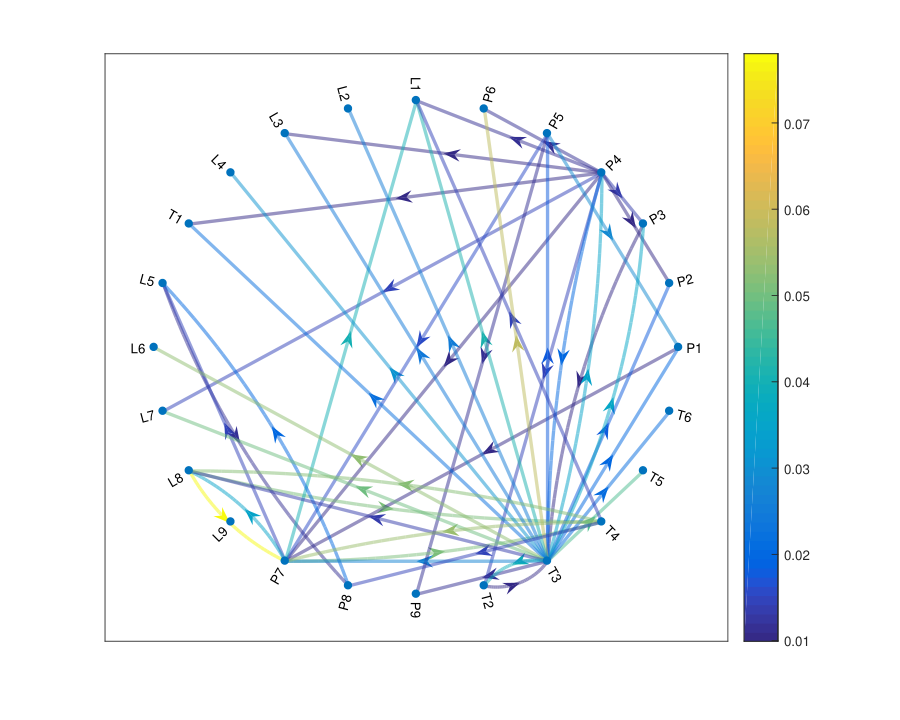
(a) NMSD vs. time
(b) NMSE1 vs. time
Fig. 7: Effect of the forgetting factor on the performance in a smooth-transition VAR model (κ=0.99\kappa=0.99, TB=1000T_{B}=1000, N=12N=12, P=2P=2, pe=0.2p_{e}=0.2, 300 Monte Carlo runs).
(a) NMSD vs. time
(b) NMSE1 vs. time
Fig. 8: Effect of the regularization parameter on the performance in a smooth-transition VAR model (κ=0.99\kappa=0.99, TB=1000T_{B}=1000, N=12N=12, T=3000T=3000 P=2P=2, pe=0.2p_{e}=0.2, γ=0.98\gamma=0.98, 200 Monte Carlo runs).
Fig. 9: Prediction NMSE vs. prediction horizon for individual variables of oil, gas, and water separation system. TIRSO is used with P=8P=8, γ=0.9\gamma=0.9, T=4T=4 hours, sampling interval = 10 s. The parameter λ\lambda is selected based on minimum average NMSE.
Refer to caption
Fig. 10: The estimated topology of a subset of the variables. The sampling interval is set to 10 seconds. The topology is obtained via TIRSO with γ=0.9\gamma=0.9, T=3T=3 hours, and P=8P=8. The parameter λ\lambda is selected based on minimum average NMSE.

Here, the step size is set to αt=1/(λmax​(𝚽⁡[t]))\alpha_{t}\!=\!1/(\lambda_{\max}(\bm{\Phi}[t])) and the NMSE is defined as NMSEh=1/(∑t∥𝒚[t+h]∥22)∑t‖𝒚[t+h]−𝒚^[t+h|t]‖22.\text{NMSE}_{h}=1/(\sum_{t}\lVert\bm{y}[t+h]\lVert_{2}^{2})\sum_{t}\left\lVert\bm{y}[t+h]-\hat{\bm{y}}[t+h|t]\right\rVert_{2}^{2}.

Fig. 9 shows the NMSEh\text{NMSE}_{h} vs. the prediction horizon hh for the time series in the data set. The temperature, pressure, and oil level time series are respectively denoted by T, P, and L and an identifying index. As expected, the prediction error increases with hh. The NMSE ranges from 10−410^{-4} to 11 due to the different predictability of each time series.

Fig. 10 presents the graph obtained by thresholding the average coefficient estimates over a three-hour duration. The threshold is such that the number of reported edges is 4​N4N. Self-loops are omitted for clarity, and arrow colors encode edge weights. It is observed that most identified edges connect sensors within each subsystem.

VI Conclusions

Two online algorithms were proposed for identifying and tracking VAR-causality graphs from time series. These algorithms sequentially accommodate data and refine their sparse topology estimates accordingly. The proposed algorithms offer complementary benefits: whereas TISO is computationally simpler, TIRSO showcases improved tracking behavior. Performance is assessed theoretically and empirically. Asymptotic equivalence of the hindsight solutions of the proposed algorithms is established and sublinear regret bounds are derived. Experiments with synthetic and real data validate the conclusions of the theoretical analysis. Future directions include explicitly modeling the variations in the VAR coefficients, possibly along the lines of [57, 58, 59], as well as identifying topologies whose adjacency matrix has a low-rank plus sparse structure along the lines of [60] to account for clusters.

References

  • [1] B. Zaman, L. M. López-Ramos, D. Romero, and B. Beferull-Lozano, “Online topology estimation for vector autoregressive processes in data networks,” in Proc. IEEE Int. Workshop Comput. Advan. Multi-Sensor Adapt. Process., Curaçao, Dutch Antilles, Dec. 2017.
  • [2] E. D. Kolaczyk, Statistical Analysis of Network Data: Methods and Models, Springer, New York, 2009.
  • [3] E. Isufi, A. Loukas, N. Perraudin, and G. Leus, “Forecasting time series with varma recursions on graphs,” arXiv preprint arXiv:1810.08581, 2018.
  • [4] P. Di Lorenzo, S. Barbarossa, P. Banelli, and S. Sardellitti, “Adaptive least mean squares estimation of graph signals,” IEEE Trans. Signal Info. Process. Netw., vol. 2, no. 4, pp. 555–568, Dec. 2016.
  • [5] C. Liu, S. Ghosal, Z. Jiang, and S. Sarkar, “An unsupervised spatiotemporal graphical modeling approach to anomaly detection in distributed CPS,” in ACM/IEEE Int. Conf. Cyber-Physical Syst., Apr. 2016, pp. 1–10.
  • [6] Y. Shen, P. A. Traganitis, and G. B. Giannakis, “Nonlinear dimensionality reduction on graphs,” in Proc. IEEE Int. Workshop Comput. Advan. Multi-Sensor Adapt. Process., Curacao, Netherlands Antilles, Dec. 2017.
  • [7] C. M. Bishop, Pattern Recognition and Machine Learning, Information Science and Statistics. Springer, 2006.
  • [8] G. Mateos, S. Segarra, A. G. Marques, and A. Ribeiro, “Connecting the dots: Identifying network structure via graph signal processing,” arXiv preprint arXiv:1810.13066, 2018.
  • [9] D. Angelosante and G. B. Giannakis, “Sparse graphical modeling of piecewise-stationary time series,” in Proc. IEEE Int. Conf. Acoust., Speech, Signal Process., Prague, Czech Republic, 2011, pp. 1960–1963.
  • [10] J. Friedman, T. Hastie, and R. Tibshirani, “Sparse inverse covariance estimation with the graphical lasso,” Biostatistics, vol. 9, no. 3, pp. 432–441, 2008.
  • [11] S. L. Lauritzen, Graphical Models, vol. 17, Clarendon Press, 1996.
  • [12] X. Dong, D. Thanou, P. Frossard, and P. Vandergheynst, “Learning Laplacian matrix in smooth graph signal representations,” IEEE Trans. Signal Process., vol. 64, no. 23, pp. 6160–6173, Dec. 2016.
  • [13] S. Segarra, A. G. Marques, G. Mateos, and A. Ribeiro, “Network topology inference from spectral templates,” IEEE Trans. Signal Info. Process. Netw., vol. 3, no. 3, pp. 467–483, Sep. 2017.
  • [14] R. B. Kline, Principles and Practice of Structural Equation Modeling, Guilford Publications, 2015.
  • [15] Y. Shen, B. Baingana, and G. B. Giannakis, “Tensor decompositions for identifying directed graph topologies and tracking dynamic networks,” IEEE Trans. Signal Process., vol. 65, no. 14, pp. 3675–3687, Jul. 2017.
  • [16] C. W. J. Granger, “Some recent development in a concept of causality,” J. Econometrics, vol. 39, no. 1-2, pp. 199–211, Sep. 1988.
  • [17] A. Zellner, “Causality and econometrics,” in Carnegie-Rochester Conference series on Public Policy. Elsevier, 1979, vol. 10, pp. 9–54.
  • [18] S. M. Kay, Fundamentals of Statistical Signal Processing, Vol. I: Estimation Theory, Prentice-Hall, 1993.
  • [19] R. Goebel, A. Roebroeck, D.S. Kim, and E. Formisano, “Investigating directed cortical interactions in time-resolved fmri data using vector autoregressive modeling and Granger causality mapping,” Magnet. Reson. Imag., vol. 21, no. 10, pp. 1251–1261, 2003.
  • [20] S. Basu, A. Shojaie, and G. Michailidis, “Network Granger causality with inherent grouping structure.,” J. Mach. Learn. Res., vol. 16, no. 2, pp. 417–453, Mar. 2015.
  • [21] A. Tank, I. Covert, N. Foti, A. Shojaie, and E. Fox, “Neural Granger causality for nonlinear time series,” arXiv preprint arXiv:1802.05842, 2018.
  • [22] H. Lütkepohl, New Introduction to Multiple Time Series Analysis, Springer, 2005.
  • [23] J. L. Lions, Optimal Control of Systems Governed by Partial Differential Equations, vol. 170, Springer Berlin, 1971.
  • [24] H. Lütkepohl, M. Krätzig, and P. CB Phillips, Applied Time Series Econometrics, Cambridge University Press, 2004.
  • [25] A. Fujita, J. R. Sato, H. M. Garay-Malpartida, R. Yamaguchi, S. Miyano, M. C. Sogayar, and C. E. Ferreira, “Modeling gene expression regulatory networks with the sparse vector autoregressive model,” BMC Syst. Bio., vol. 1, no. 1, pp. 39, 2007.
  • [26] P. A. Valdés-Sosa, J. M. Sánchez-Bornot, A. Lage-Castellanos, M. Vega-Hernández, J. Bosch-Bayard, L. Melie-García, and E. Canales-Rodríguez, “Estimating brain functional connectivity with sparse multivariate autoregression,” Philosoph. Trans. Royal Soc. London B: Bio. Sci., vol. 360, no. 1457, pp. 969–981, 2005.
  • [27] F. R. Bach and M. I. Jordan, “Learning graphical models for stationary time series,” IEEE Trans. Signal Process., vol. 52, no. 8, pp. 2189–2199, Aug. 2004.
  • [28] J. Songsiri and L. Vandenberghe, “Topology selection in graphical models of autoregressive processes,” J. Mach. Learn. Res., vol. 11, pp. 2671–2705, Oct. 2010.
  • [29] A. Bolstad, B. D. Van Veen, and R. Nowak, “Causal network inference via group sparse regularization,” IEEE Trans. Signal Process., vol. 59, no. 6, pp. 2628–2641, Jun. 2011.
  • [30] J. Songsiri, “Sparse autoregressive model estimation for learning Granger causality in time series,” in Proc. IEEE Int. Conf. Acoust., Speech, Signal Process., Vancouver, BC, May 2013, pp. 3198–3202.
  • [31] J. Mei and J. M. F. Moura, “Signal processing on graphs: Causal modeling of unstructured data,” IEEE Trans. Signal Process., vol. 65, no. 8, pp. 2077–2092, Apr. 2017.
  • [32] M. Ayazoglu, M. Sznaier, and N. Ozay, “Blind identification of sparse dynamic networks and applications,” in IEEE Conf. Decision Control Eur. Control Conf., 2011, pp. 2944–2950.
  • [33] M. Kolar, L. Song, A. Ahmed, and E. P. Xing, “Estimating time-varying networks,” Ann. Appl. Statist, pp. 94–123, 2010.
  • [34] J. Lee, G. Li, and J. D. Wilson, “Varying-coefficient models for dynamic networks,” arXiv preprint arXiv:1702.03632, 2017.
  • [35] L. M. Lopez-Ramos, D. Romero, B. Zaman, and B. Beferull-Lozano, “Dynamic network identification from non-stationary vector autoregressive time series,” in Proc. IEEE Global Conf. Signal Inf. Process., 2018, pp. 773–777.
  • [36] D. Hallac, Y. Park, S. Boyd, and J. Leskovec, “Network inference via the time-varying graphical lasso,” in Proc. ACM SIGKDD Int. Conf. Knowl. Discov. Data Min., 2017, pp. 205–213.
  • [37] B. Baingana, G. Mateos, and G. B. Giannakis, “Proximal-gradient algorithms for tracking cascades over social networks,” IEEE J. Sel. Topics Signal Process., vol. 8, no. 4, pp. 563–575, Aug. 2014.
  • [38] M. G. Rodriguez, J. Leskovec, and B. Schölkopf, “Structure and dynamics of information pathways in online media,” in Proc. ACM Int. Conf. Web Search Data Mining, 2013, pp. 23–32.
  • [39] B. Zaman, L. M. Lopez-Ramos, and B. Beferull-Lozano, “Dynamic regret analysis for online tracking of time-varying structural equation model topologies,” arXiv preprint arXiv:2003.08145, 2020.
  • [40] R. Shafipour, A. Hashemi, G. Mateos, and H. Vikalo, “Online topology inference from streaming stationary graph signals,” in IEEE Data Sci. Workshop, Jun. 2019, pp. 140–144.
  • [41] Y. Shen and G. B. Giannakis, “Online identification of directional graph topologies capturing dynamic and nonlinear dependencies,” in IEEE Data Sci. Workshop, 2018, pp. 195–199.
  • [42] J. Duchi, S. Shalev-Shwartz, Y. Singer, and A. Tewari, “Composite objective mirror descent,” in Proc. of Annu. Conf. Computat. Learn. Theory, 2010, pp. 14–26.
  • [43] E. M. Eksioglu and A K. Tanc, “RLS algorithm with convex regularization,” IEEE Signal Process. Lett., vol. 18, no. 8, pp. 470–473, Aug. 2011.
  • [44] M. Yuan and Y. Lin, “Model selection and estimation in regression with grouped variables,” J. Royal Statist. Soc.: Series B (Statist. Method.), vol. 68, no. 1, pp. 49–67, 2006.
  • [45] H. Liu and J. Zhang, “Estimation consistency of the group lasso and its applications,” in Artificial Intell. and Stat., 2009, pp. 376–383.
  • [46] S. Shalev-Shwartz, “Online learning and online convex optimization,” Found. Trends Mach. Learn., vol. 4, no. 2, pp. 107–194, 2011.
  • [47] E. C. Hall and R. M. Willett, “Online convex optimization in dynamic environments,” IEEE J. Sel. Topics Signal Process., vol. 9, no. 4, pp. 647–662, Jun. 2015.
  • [48] E. Hazan, “Introduction to online convex optimization,” Found. Trends Mach. Learn., vol. 2, no. 3-4, pp. 157–325, 2016.
  • [49] A. Mokhtari, S. Shahrampour, A. Jadbabaie, and A. Ribeiro, “Online optimization in dynamic environments: Improved regret rates for strongly convex problems,” arXiv preprint arXiv:1603.04954, 2016.
  • [50] L. Xiao, “Dual averaging methods for regularized stochastic learning and online optimization,” J. Mach. Learn. Res., vol. 11, pp. 2543–2596, 2010.
  • [51] A. T. Puig, A. Wiesel, G. Fleury, and A. O. Hero, “Multidimensional shrinkage-thresholding operator and group lasso penalties,” IEEE Signal Process. Lett., vol. 18, no. 6, pp. 363–366, Jun. 2011.
  • [52] A. H. Sayed, Fundamentals of Adaptive Filtering, John Wiley & Sons, 2003.
  • [53] S. M. Fosson, “Online optimization in dynamic environments: A regret analysis for sparse problems,” in IEEE Conf. Decision Control, Dec. 2018, pp. 7225–7230.
  • [54] R. Dixit, A. S. Bedi, R. Tripathi, and K. Rajawat, “Online learning with inexact proximal online gradient descent algorithms,” IEEE Trans. Signal Process., vol. 67, no. 5, pp. 1338–1352, Mar. 2019.
  • [55] G. B. Giannakis, Y. Shen, and G. V. Karanikolas, “Topology identification and learning over graphs: Accounting for nonlinearities and dynamics,” Proc. IEEE, vol. 106, no. 5, pp. 787–807, May 2018.
  • [56] L. Kilian and H. Lütkepohl, Structural Vector Autoregressive Analysis, Cambridge University Press, 2017.
  • [57] Y. I. Abramovich, N. K. Spencer, and M. D. E. Turley, “Time-varying autoregressive (TVAR) adaptive order and spectrum estimation,” in Proc. Asilomar Conf. Signal, Syst., Comput., Pacific Grove, CA, 2005.
  • [58] Y. I. Abramovich, N. K. Spencer, and M. D. E. Turley, “Order estimation and discrimination between stationary and time-varying (TVAR) autoregressive models,” IEEE Trans. Signal Process., vol. 55, no. 6, pp. 2861–2876, Jun. 2007.
  • [59] S. Lundbergh, T. Teräsvirta, and D. V. Dijk, “Time-varying smooth transition autoregressive models,” J. Bus. Econ. Stat., vol. 21, no. 1, pp. 104–121, Jan. 2003.
  • [60] T. Kanada, M. Onuki, and Y. Tanaka, “Low-rank sparse decomposition of graph adjacency matrices for extracting clean clusters,” in Asia-Pacific Signal Inf. Process. Assoc. Annu. Summit Conf., 2018, pp. 1153–1159.
  • [61] S. Boyd and L. Vandenberghe, Convex Optimization, Cambridge University Press, Cambridge, UK, 2004.
  • [62] C. D. Meyer, Matrix Analysis and Applied Linear Algebra, vol. 71, Siam, 2000.
  • [63] R. A. Horn and C. R. Johnson, Matrix Analysis, Cambridge Univ. Press, Cambridge, U.K., 1985.
  • [64] G. H. Golub, C. F. Van Loan, C. F. Van Loan, and P. C. F. Van Loan, Matrix Computations, The Johns Hopkins Univ. Press, 1996.
  • [65] N. Parikh and S. Boyd, “Proximal algorithms,” Found. Trends Optim., vol. 1, no. 3, pp. 127–239, 2014.

Supplementary Material

Appendix A Proof of ?THM? 

The first step is to rewrite (30) to be able to obtain a simple expression for CT​(𝒂n)−C~T​(𝒂n){\color[rgb]{0,0,0}C}_{T}(\bm{a}_{n})-{\color[rgb]{0,0,0}\tilde{C}}_{T}(\bm{a}_{n}). To this end, substitute (19) into (30) and exchange the order of the summations to obtain

C~T​(𝒂n)\displaystyle{\color[rgb]{0,0,0}\tilde{C}}_{T}(\bm{a}_{n}) =1T−P​∑τ=PT−1[∑t=τT−1γt−τ​μ​ℓτ(n)​(𝒂n)+λ​∑n′=1n′≠nN‖𝒂n,n′‖2]\displaystyle=\textstyle\frac{1}{T-P}\displaystyle\sum_{\tau=P}^{T-1}\Big[\sum_{t=\tau}^{T-1}\gamma^{t-\tau}\mu\,\ell_{\tau}^{(n)}(\bm{a}_{n})+\lambda\sum_{\begin{subarray}{c}n^{\prime}=1\\ n^{\prime}\neq n\end{subarray}}^{N}\left\lVert\bm{a}_{n,n^{\prime}}\right\rVert_{2}\Big]
=1T−P​∑τ=PT−1θτ,T​μ​ℓτ(n)​(𝒂n)+λ​∑n′=1,n′≠nN‖𝒂n,n′‖2,\displaystyle=\textstyle\frac{1}{T-P}\displaystyle\sum_{\tau=P}^{T-1}{\theta_{\tau,T}}\,\mu\,\ell_{\tau}^{(n)}(\bm{a}_{n})+\lambda\sum_{\begin{subarray}{c}n^{\prime}=1,n^{\prime}\neq n\end{subarray}}^{N}\left\lVert\bm{a}_{n,n^{\prime}}\right\rVert_{2},

where θτ,T≜∑t=τT−1γt−τ\theta_{\tau,T}\triangleq\sum_{t=\tau}^{T-1}\gamma^{t-\tau}. From the geometric series summation formula, which establishes that θτ,T=(1−γT−τ)/(1−γ)\theta_{\tau,T}=({1-\gamma^{T-\tau}})/({1-\gamma}), and noting that μ=1−γ\mu=1-\gamma, the above equation becomes

C~T​(𝒂n)=1T−P​∑τ=PT−1(1−γT−τ)​ℓτ(n)​(𝒂n)+λ​∑n′=1n′≠nN‖𝒂n,n′‖2.{\color[rgb]{0,0,0}\tilde{C}}_{T}(\bm{a}_{n})=\textstyle\frac{1}{T-P}\displaystyle\sum_{\tau=P}^{T-1}(1-\gamma^{T-\tau})\,\ell_{\tau}^{(n)}(\bm{a}_{n})+\lambda\sum_{\begin{subarray}{c}n^{\prime}=1\\ n^{\prime}\neq n\end{subarray}}^{N}\left\lVert\bm{a}_{n,n^{\prime}}\right\rVert_{2}.

From (28) and the equation above, the difference dT​(𝒂n)≜CT​(𝒂n)−C~T​(𝒂n)d_{T}(\bm{a}_{n})\triangleq{\color[rgb]{0,0,0}C}_{T}(\bm{a}_{n})-{\color[rgb]{0,0,0}\tilde{C}}_{T}(\bm{a}_{n}) between the TISO and TIRSO hindsight objectives is given by:

dT​(𝒂n)\displaystyle d_{T}(\bm{a}_{n}) =1T−P​∑τ=PT−1γT−τ​ℓτ(n)​(𝒂n).\displaystyle=\textstyle\frac{1}{T-P}\sum_{\tau=P}^{T-1}\gamma^{T-\tau}\,\ell_{\tau}^{(n)}(\bm{a}_{n}). (45)

To prove part 1, it suffices to show that dT​(𝒂n)→0d_{T}(\bm{a}_{n})\rightarrow 0 as T→∞T\rightarrow\infty for all 𝒂n\bm{a}_{n}. To this end, expand ℓt(n)​(𝒂n)\ell_{t}^{(n)}(\bm{a}_{n})

ℓt(n)​(𝒂n)=12​(yn2​[t]+𝒂n⊤​𝒈​[t]​𝒈⊤​[t]​𝒂n−2​yn​[t]​𝒈⊤​[t]​𝒂n),\displaystyle\ell_{t}^{(n)}(\bm{a}_{n})\!=\!\frac{1}{2}\left(y_{n}^{2}[t]+\bm{a}_{n}^{\top}\,\bm{g}[t]\,\bm{g}^{\top}[t]\,\bm{a}_{n}\!-\!2\,y_{n}[t]\,\bm{g}^{\top}[t]\,\bm{a}_{n}\right), (46)

and apply Cauchy-Schwarz inequality to obtain

ℓt(n)​(𝒂n)≤12​[‖𝒂n‖2⋅‖𝒈⁡[t]‖2]2+12​By+By​‖𝒈⁡[t]‖2⋅‖𝒂n‖2.\displaystyle\ell_{t}^{(n)}(\bm{a}_{n})\!\leq\!\frac{1}{2}\left[\left\lVert\bm{a}_{n}\right\rVert_{2}\cdot\left\lVert\bm{g}[t]\right\rVert_{2}\right]^{2}\!+\!\frac{1}{2}{\color[rgb]{0,0,0}B}_{y}\!+\!\sqrt{{\color[rgb]{0,0,0}B}_{y}}\left\lVert\bm{g}[t]\right\rVert_{2}\cdot\left\lVert\bm{a}_{n}\right\rVert_{2}. (47)

On the other hand, the hypothesis |yn​[t]|2≤By​∀n,t|y_{n}[t]|^{2}\leq{\color[rgb]{0,0,0}B}_{y}\forall n,t implies that ∥𝒚⁡[t]∥22≤N​By\lVert\bm{y}[t]\rVert_{2}^{2}\leq N{\color[rgb]{0,0,0}B}_{y}, and hence

‖𝒈⁡[t]‖22=∑τ=t−Pt−1‖𝒚⁡[τ]‖22≤P​maxt−P≤τ≤t−1​‖𝒚⁡[τ]‖22≤P​N​By.\left\lVert\bm{g}[t]\right\rVert_{2}^{2}\!=\sum_{\tau=t-P}^{t-1}\left\lVert\bm{y}[\tau]\right\rVert_{2}^{2}\leq P\!\underset{t-P\leq\tau\leq t-1}{\text{max}}\!\left\lVert\bm{y}[\tau]\right\rVert_{2}^{2}\leq PN{\color[rgb]{0,0,0}B}_{y}.

Substituting the upper bound of ∥𝒈⁡[t]∥22\lVert\bm{g}[t]\rVert_{2}^{2} into (47) yields

ℓt(n)​(𝒂n)\displaystyle\ell_{t}^{(n)}(\bm{a}_{n}) ≤12​N​P​By​‖𝒂n‖22+12​By+N​P​By​‖𝒂n‖2≜G⁡(𝒂n)\displaystyle\leq\frac{1}{2}NP{\color[rgb]{0,0,0}B}_{y}\left\lVert\bm{a}_{n}\right\rVert_{2}^{2}+\!\frac{1}{2}{\color[rgb]{0,0,0}B}_{y}\!+\!\sqrt{NP}{\color[rgb]{0,0,0}B}_{y}\left\lVert\bm{a}_{n}\right\rVert_{2}\triangleq G(\bm{a}_{n}) (48)

Applying the latter bound to (45) results in

dT​(𝒂n)\displaystyle d_{T}(\bm{a}_{n}) ≤1T−P​∑τ=PT−1γT−τ​G​(𝒂n)\displaystyle\leq\frac{1}{T-P}\sum_{\tau=P}^{T-1}\gamma^{T-\tau}\,G(\bm{a}_{n})
=G⁡(𝒂n)​γTT−P​∑τ=PT−1γ−τ=G⁡(𝒂n)​(1−γT−P)(T−P)​(γ−1−1).\displaystyle=\frac{G(\bm{a}_{n})\gamma^{T}}{T-P}\sum_{\tau=P}^{T-1}\gamma^{-\tau}=\frac{G(\bm{a}_{n})\left(1-\gamma^{T-P}\right)}{(T-P)(\gamma^{-1}-1)}. (49)

Taking the limit of the right-hand side clearly yields

limT→∞G⁡(𝒂n)​(1−γT−P)(T−P)​(γ−1−1)=0.\lim\limits_{T\rightarrow\infty}\frac{G(\bm{a}_{n})\left(1-\gamma^{T-P}\right)}{(T-P)(\gamma^{-1}-1)}=0. (50)

Noting from (45) that dT​(𝒂n)≥0d_{T}(\bm{a}_{n})\geq 0, it follows that limT→∞dT​(𝒂n)=0\lim_{T\rightarrow\infty}d_{T}(\bm{a}_{n})=0, which concludes the proof of part 1.

To prove part 2, note from (45) that dT​(𝒂n)≥0d_{T}(\bm{a}_{n})\geq 0, which in turn implies that

C~T​(𝒂n)≤CT​(𝒂n),{\color[rgb]{0,0,0}\tilde{C}}_{T}(\bm{a}_{n})\leq{\color[rgb]{0,0,0}C}_{T}(\bm{a}_{n}), (51)

for all 𝒂n\bm{a}_{n} and T>PT>P. On the other hand, it follows from (29) that

C~T​(𝒂~n∗​[T])≤C~T​(𝒂n∗​[T]).{\color[rgb]{0,0,0}\tilde{C}}_{T}({\tilde{\bm{a}}}_{n}^{*}[T])\leq{\color[rgb]{0,0,0}\tilde{C}}_{T}(\bm{a}_{n}^{*}[T]). (52)

Thus, by combining (51) and (52),

C~T​(𝒂~n∗​[T])≤CT​(𝒂n∗​[T]).{\color[rgb]{0,0,0}\tilde{C}}_{T}({\tilde{\bm{a}}}_{n}^{*}[T])\leq{\color[rgb]{0,0,0}C}_{T}(\bm{a}_{n}^{*}[T]). (53)

Similarly, from (27), it holds that CT​(𝒂n∗​[T])≤CT​(𝒂~n∗​[T]){\color[rgb]{0,0,0}C}_{T}(\bm{a}_{n}^{*}[T])\leq{\color[rgb]{0,0,0}C}_{T}({\tilde{\bm{a}}}_{n}^{*}[T]). Subtracting C~T​(𝒂~n∗​[T]){\color[rgb]{0,0,0}\tilde{C}}_{T}({\tilde{\bm{a}}}_{n}^{*}[T]) from both sides of the latter inequality yields

CT​(𝒂n∗​[T])−C~T​(𝒂~n∗​[T])≤CT​(𝒂~n∗​[T])−C~T​(𝒂~n∗​[T])\displaystyle{\color[rgb]{0,0,0}C}_{T}(\bm{a}_{n}^{*}[T])-{\color[rgb]{0,0,0}\tilde{C}}_{T}({\tilde{\bm{a}}}_{n}^{*}[T])\leq{\color[rgb]{0,0,0}C}_{T}({\tilde{\bm{a}}}_{n}^{*}[T])-{\color[rgb]{0,0,0}\tilde{C}}_{T}({\tilde{\bm{a}}}_{n}^{*}[T])
=dT​(𝒂~n∗​[T]).\displaystyle=d_{T}({\tilde{\bm{a}}}_{n}^{*}[T]). (54)

By combining (53) and (A), it holds that

0≤CT​(𝒂n∗​[T])−C~T​(𝒂~n∗​[T])≤dT​(𝒂~n∗​[T]).0\leq{\color[rgb]{0,0,0}C}_{T}(\bm{a}_{n}^{*}[T])-{\color[rgb]{0,0,0}\tilde{C}}_{T}({\tilde{\bm{a}}}_{n}^{*}[T])\leq d_{T}({\tilde{\bm{a}}}_{n}^{*}[T]). (55)

Since limT→∞dT​(𝒂~n∗​[T])=0\lim_{T\rightarrow\infty}d_{T}({\tilde{\bm{a}}}_{n}^{*}[T])=0, (55) implies that

limT→∞CT​(𝒂n∗​[T])−C~T​(𝒂~n∗​[T])=0.\lim_{T\rightarrow\infty}{\color[rgb]{0,0,0}C}_{T}(\bm{a}_{n}^{*}[T])-{\color[rgb]{0,0,0}\tilde{C}}_{T}({\tilde{\bm{a}}}_{n}^{*}[T])=0. (56)

Finally, to establish part 3, note that it follows from assumption A2, (20) and (30) that C~T{\color[rgb]{0,0,0}\tilde{C}}_{T} is β~\tilde{\beta}-strongly convex for some β~>0,∀T\tilde{\beta}>0,\forall\,T. Thus, from (29), one finds that

C~T​(𝒂n∗​[T])≥C~T​(𝒂~n∗​[T])+β~2​‖𝒂n∗​[T]−𝒂~n∗​[T]‖22.{\color[rgb]{0,0,0}\tilde{C}}_{T}(\bm{a}_{n}^{*}[T])\geq{\color[rgb]{0,0,0}\tilde{C}}_{T}({\tilde{\bm{a}}}_{n}^{*}[T])+\frac{{\tilde{\beta}}}{2}\left\lVert\bm{a}_{n}^{*}[T]-{\tilde{\bm{a}}}_{n}^{*}[T]\right\rVert_{2}^{2}. (57)

By combining (51) and (57), it follows that

CT​(𝒂n∗​[T])≥C~T​(𝒂~n∗​[T])+β~2​‖𝒂n∗​[T]−𝒂~n∗​[T]‖22,{\color[rgb]{0,0,0}C}_{T}(\bm{a}_{n}^{*}[T])\geq{\color[rgb]{0,0,0}\tilde{C}}_{T}({\tilde{\bm{a}}}_{n}^{*}[T])+\frac{{\tilde{\beta}}}{2}\left\lVert\bm{a}_{n}^{*}[T]-{\tilde{\bm{a}}}_{n}^{*}[T]\right\rVert_{2}^{2}, (58)

or, equivalently,

CT​(𝒂n∗​[T])−C~T​(𝒂~n∗​[T])≥β~2​‖𝒂n∗​[T]−𝒂~n∗​[T]‖22≥0.{\color[rgb]{0,0,0}C}_{T}(\bm{a}_{n}^{*}[T])-{\color[rgb]{0,0,0}\tilde{C}}_{T}({\tilde{\bm{a}}}_{n}^{*}[T])\geq\frac{{\tilde{\beta}}}{2}\left\lVert\bm{a}_{n}^{*}[T]-{\tilde{\bm{a}}}_{n}^{*}[T]\right\rVert_{2}^{2}\geq 0. (59)

Taking limits gives rise to

limT→∞[CT(𝒂n∗[T])−C~T(𝒂~n∗[T])]≥limT→∞[β~2∥𝒂n∗[T]−𝒂~n∗[T]∥22]≥0.\hskip-14.22636pt\lim_{T\rightarrow\infty}\big[{\color[rgb]{0,0,0}C}_{T}(\bm{a}_{n}^{*}[T])-{\color[rgb]{0,0,0}\tilde{C}}_{T}({\tilde{\bm{a}}}_{n}^{*}[T])\big]\geq\lim_{T\rightarrow\infty}\Big[\frac{{\tilde{\beta}}}{2}\lVert\bm{a}_{n}^{*}[T]\\ -{\tilde{\bm{a}}}_{n}^{*}[T]\rVert_{2}^{2}\Big]\geq 0. (60)

From (56) and the sandwich theorem applied to (60), we have

limT→∞[β~2​∥𝒂n∗​[T]−𝒂~n∗​[T]∥22]=0,\lim_{T\rightarrow\infty}\Big[\frac{{\tilde{\beta}}}{2}\lVert\bm{a}_{n}^{*}[T]-{\tilde{\bm{a}}}_{n}^{*}[T]\rVert_{2}^{2}\Big]=0, (61)

which concludes the proof.

Appendix B Proof of ?THM? 

Consider first the regret of TISO with constant step size.

Lemma 1.

Let {𝐚n​[t]}t=PT\{\bm{a}_{n}[t]\}_{t=P}^{T} be generated by TISO (Procedure 1) with constant step size αt=α=𝒪⁡(1/T)\alpha_{t}\!=\alpha\!=\!\mathcal{O}\big(1/\sqrt{T}\big). Under assumptions A1 and A26, we have

R[T](n)s=𝒪(PNByB𝒂2T).\displaystyle R{{}_{s}^{(n)}[T]}=\mathcal{O}\left(PN{\color[rgb]{0,0,0}B}_{y}\,{B_{\bm{a}}^{2}}\,\sqrt{T}\right). (62)
Proof:

See Appendix C. ∎Observe that the step size in ?THM?  depends on TT and therefore (62) cannot be interpreted as directly establishing sublinear regret for TISO. To understand this result, consider a sequence of copies of TISO, each one for a value of TT. Each copy has a (potentially) different step size, but uses the same step size for all tt. Expression (62) bounds the regret of the TT-th copy at time TT. However, ?THM?  can be used next to establish sublinear regret for step size sequences that remain constant over windows of exponentially increasing length; see the doubling trick [46].

To this end, let the regret in the window [t1,t2][t_{1},t_{2}] be

Rs(n)​[t1,t2]≜∑t=t1t2ht(n)​(𝒂n​[t])−ht(n)​(𝒂n∗​[t1,t2]),R_{s}^{(n)}[t_{1},t_{2}]\triangleq\sum_{t=t_{1}}^{t_{2}}h_{t}^{(n)}(\bm{a}_{n}[t])-h_{t}^{(n)}(\bm{a}_{n}^{*}[t_{1},t_{2}]), (63)

where {𝒂n​[t]}t⊂ℝN​P\{\bm{a}_{n}[t]\}_{t}\subset\mathbb{R}^{NP} is an arbitrary sequence and

𝒂n∗[t1,t2]≜arg​min𝐚n∑t=t1t2ht(n)(𝐚n).\bm{a}_{n}^{*}[t_{1},t_{2}]\triangleq\argmin_{\bm{a}_{n}}\sum_{t=t_{1}}^{t_{2}}h_{t}^{(n)}(\bm{a}_{n}). (64)

The next result establishes a bound on the static regret given the regret at each window.

Lemma 2.

For T=t0​2MT=t_{0}2^{M} and for an arbitrary sequence {𝐚n​[t]}t⊂ℝN​P\{\bm{a}_{n}[t]\}_{t}\subset\mathbb{R}^{NP}, the regret in (31) is bounded as:

Rs(n)​[T]≤Rs(n)​[P,t0]+∑m=1MRs(n)​[t0​2m−1+1,t0​2m].\displaystyle R_{s}^{(n)}[T]\leq R_{s}^{(n)}[P,t_{0}]+\sum_{m=1}^{M}R_{s}^{(n)}[t_{0}2^{m-1}\!\!+\!1,t_{0}2^{m}]. (65)
Proof:

For T=t0​2MT=t_{0}2^{M}, expression (31) can be written as:

Rs(n)​[T]\displaystyle R_{s}^{(n)}[T] =∑t=Pt0​2Mht(n)​(𝒂n​[t])−∑t=Pt0​2Mht(n)​(𝒂n∗​[T]).\displaystyle=\sum_{t=P}^{t_{0}2^{M}}h_{t}^{(n)}(\bm{a}_{n}[t])-\sum_{t=P}^{t_{0}2^{M}}h_{t}^{(n)}\left(\bm{a}_{n}^{*}[T]\right). (66)

On the other hand, it follows from (63) that (65) is equivalent to

Rs(n)​[T]≤∑t=Pt0[ht(n)​(𝒂n​[t])−ht(n)​(𝒂n∗​[P,t0])]\displaystyle R_{s}^{(n)}[T]\leq\sum_{t=P}^{t_{0}}\left[h_{t}^{(n)}(\bm{a}_{n}[t])-h_{t}^{(n)}\left(\bm{a}_{n}^{*}[P,t_{0}]\right)\right]
+∑m=1M∑t=t0​2m−1+1t0​2m[ht(n)(𝒂n[t])−ht(n)(𝒂n∗[t02m−1+1,t02m])],\displaystyle+\sum_{m=1}^{M}\sum_{t=t_{0}2^{m-1}+1}^{t_{0}2^{m}}\!\!\!\!\left[h_{t}^{(n)}\!(\bm{a}_{n}[t])\!-\!h_{t}^{(n)}\left(\bm{a}_{n}^{*}\left[t_{0}2^{m-1}\!\!+\!1,t_{0}2^{m}\right]\right)\right], (67)

The inequality in (67) can also be rewritten as

Rs(n)​[T]\displaystyle R_{s}^{(n)}[T] ≤∑t=Pt0​2Mht(n)(𝒂n[t])−[∑t=Pt0ht(n)(𝒂n∗[P,t0])\displaystyle\leq\sum_{t=P}^{t_{0}2^{M}}h_{t}^{(n)}(\bm{a}_{n}[t])-\bigg[\sum_{t=P}^{t_{0}}h_{t}^{(n)}\left(\bm{a}_{n}^{*}[P,t_{0}]\right)
+∑m=1M∑t=t0​2m−1+1t0​2mht(n)(𝒂n∗[t02m−1+1,t02m])].\displaystyle\quad+\sum_{m=1}^{M}\sum_{t=t_{0}2^{m-1}+1}^{t_{0}2^{m}}h_{t}^{(n)}\left(\bm{a}_{n}^{*}\left[t_{0}2^{m-1}\!\!+\!1,t_{0}2^{m}\right]\right)\bigg]. (68)

By comparing (66) and (68), proving (65) is equivalent to showing that

∑t=Pt0​2Mht(n)(𝒂n∗[T])≥[∑t=Pt0ht(n)(𝒂n∗[P,t0])+∑m=1M∑t=t0​2m−1+1t0​2mht(n)(𝒂n∗[t02m−1+1,t02m])].\sum_{t=P}^{t_{0}2^{M}}h_{t}^{(n)}\left(\bm{a}_{n}^{*}[T]\right)\geq\bigg[\sum_{t=P}^{t_{0}}h_{t}^{(n)}\left(\bm{a}_{n}^{*}[P,t_{0}]\right)+\\ \sum_{m=1}^{M}\sum_{t=t_{0}2^{m-1}+1}^{t_{0}2^{m}}h_{t}^{(n)}\left(\bm{a}_{n}^{*}\left[t_{0}2^{m-1}\!\!+\!1,t_{0}2^{m}\right]\right)\bigg]. (69)

From the definitions of 𝒂n∗​[T]\bm{a}_{n}^{*}[T] in (27) and 𝒂n∗​[t1,t2]\bm{a}_{n}^{*}[t_{1},t_{2}] in (64), the above inequality holds since inf𝒙,𝒚f⁡(𝒙,𝒚)≤inf𝒙=𝒚f⁡(𝒙,𝒚)\inf_{\bm{x},\bm{y}}f(\bm{x},\bm{y})\leq\inf_{\bm{x}=\bm{y}}f(\bm{x},\bm{y}). ∎The next step is to bound the regret at each window using ?THM? . To this end, one must set α[m]\alpha_{[m]} as a function 𝒪⁡(1/Tm)\mathcal{O}(1/\sqrt{T_{m}}), where Tm≜t0​2m−t0​2m−1=t0​2m−1T_{m}\triangleq t_{0}2^{m}-t_{0}2^{m-1}=t_{0}2^{m-1} is the length of the (m+1)(m+1)-th window, m=1,…,Mm=1,\ldots,M. Invoking ?THM? , the regret for the (m+1)(m+1)-th window is given by Rs(n)​[t0​2m−1+1,t0​2m]=𝒪⁡(P​N​By​B𝒂2​2m−1)R_{s}^{(n)}[t_{0}2^{m-1}+1,t_{0}2^{m}]=\mathcal{O}(PN{\color[rgb]{0,0,0}B}_{y}B_{\bm{a}}^{2}\sqrt{2^{m-1}}). By ?THM? , the regret of TISO becomes

Rs(n)​[T]\displaystyle R_{s}^{(n)}[T] =𝒪⁡(P​N​By​B𝒂2​t0−P+1)\displaystyle=\mathcal{O}\left(PN{\color[rgb]{0,0,0}B}_{y}B_{\bm{a}}^{2}\sqrt{t_{0}-P+1}\right)
+∑m=1M𝒪(PNByB𝒂2t0​2m−1)\displaystyle\quad+\sum_{m=1}^{M}\mathcal{O}\left(PN{\color[rgb]{0,0,0}B}_{y}B_{\bm{a}}^{2}\sqrt{t_{0}2^{m-1}}\right)
=𝒪⁡(P​N​By​B𝒂2​∑m=1Mt0​2m−1)\displaystyle=\mathcal{O}\left(PN{\color[rgb]{0,0,0}B}_{y}B_{\bm{a}}^{2}\sum_{m=1}^{M}\sqrt{t_{0}2^{m-1}}\right)
=𝒪⁡(P​N​By​B𝒂2​(2)M)\displaystyle=\mathcal{O}\left(PN{\color[rgb]{0,0,0}B}_{y}B_{\bm{a}}^{2}(\sqrt{2})^{M}\right)
=𝒪⁡(P​N​By​B𝒂2​(2log2⁡Tt0)12)\displaystyle=\mathcal{O}\left(PN{\color[rgb]{0,0,0}B}_{y}B_{\bm{a}}^{2}\left(2^{\log_{2}\frac{T}{t_{0}}}\right)^{\frac{1}{2}}\right)
=𝒪⁡(P​N​By​B𝒂2​T),\displaystyle=\mathcal{O}\left(PN{\color[rgb]{0,0,0}B}_{y}B_{\bm{a}}^{2}\sqrt{T}\right),

which concludes the proof.

Appendix C Proof of ?THM? 

First we present a lemma that establishes that the hindsight solution of TISO is bounded and then we will present the proof of ?THM? .

Lemma 3.

Under assumptions A1, A2, and A26, the hindsight solution of TISO 𝐚n∗​[T]\bm{a}_{n}^{*}[T] given in (27) is bounded as

‖𝒂n∗​[T]‖2≤B𝒂≜1β​(By​P​N+By2​P​N+β​By).\displaystyle\left\lVert\bm{a}_{n}^{*}[T]\right\rVert_{2}\leq B_{\bm{a}}\triangleq\frac{1}{\beta}\left({\color[rgb]{0,0,0}B}_{y}\sqrt{PN}+\sqrt{{\color[rgb]{0,0,0}B}_{y}^{2}PN+\beta{\color[rgb]{0,0,0}B}_{y}}\right). (70)
Proof:

Note that an∗​[T]a_{n}^{*}[T] belongs to the sublevel set of TISO hindsight objective for 𝒂n=𝟎N​P\bm{a}_{n}=\bm{0}_{NP}, given by

𝒮T≜{𝒂n:CT​(𝒂n)≤CT​(𝟎N​P)},\mathcal{S}_{T}\triangleq\left\{\bm{a}_{n}:{\color[rgb]{0,0,0}C}_{T}(\bm{a}_{n})\leq{\color[rgb]{0,0,0}C}_{T}(\bm{0}_{NP})\right\}, (71)

where CT​(𝟎N​P){\color[rgb]{0,0,0}C}_{T}(\bm{0}_{NP}) is upper bounded by

CT​(𝟎N​P)\displaystyle{\color[rgb]{0,0,0}C}_{T}(\bm{0}_{NP}) =1T−P​∑t=PT−112​yn2​[t]\displaystyle=\frac{1}{T-P}\sum_{t=P}^{T-1}\frac{1}{2}y_{n}^{2}[t]
≤12​(T−P)​∑t=PT−1By=By2.\displaystyle\leq\frac{1}{2(T-P)}\sum_{t=P}^{T-1}{\color[rgb]{0,0,0}B}_{y}=\frac{{\color[rgb]{0,0,0}B}_{y}}{2}.

This means that we can write:

𝒮T⊂{𝒂n∗​[T]:CT​(𝒂n∗​[T])≤By2}.\mathcal{S}_{T}\subset\left\{\bm{a}_{n}^{*}[T]:{\color[rgb]{0,0,0}C}_{T}(\bm{a}_{n}^{*}[T])\leq\frac{{\color[rgb]{0,0,0}B}_{y}}{2}\right\}. (72)

Next, we find a lower bound to CT​(𝒂n∗​[T]){\color[rgb]{0,0,0}C}_{T}(\bm{a}_{n}^{*}[T]) that is an increasing function of ∥𝒂n∗​[T]∥2\lVert\bm{a}_{n}^{*}[T]\rVert_{2} as follows

CT​(𝒂n∗​[T])\displaystyle{\color[rgb]{0,0,0}C}_{T}(\bm{a}_{n}^{*}[T]) =1T−P∑t=PT−1[12(𝒂n∗[T])⊤𝒈[t]𝒈⊤[t]𝒂n∗[T]\displaystyle=\frac{1}{T-P}\sum_{t=P}^{T-1}\Big[\frac{1}{2}(\bm{a}_{n}^{*}[T])^{\top}\bm{g}[t]\bm{g}^{\top}[t]\bm{a}_{n}^{*}[T]
−yn[t]𝒈⊤[t]𝒂n∗[T]+12yn2[t]+Ω(n)(𝒂n∗[T])]\displaystyle-y_{n}[t]\bm{g}^{\top}[t]\bm{a}_{n}^{*}[T]+\frac{1}{2}y_{n}^{2}[t]+{\Omega}^{(n)}(\bm{a}_{n}^{*}[T])\Big]
≥1T−P∑t=PT−1[12(𝒂n∗[T])⊤𝒈[t]𝒈⊤[t]𝒂n∗[T]\displaystyle\geq\frac{1}{T-P}\sum_{t=P}^{T-1}\Big[\frac{1}{2}(\bm{a}_{n}^{*}[T])^{\top}\bm{g}[t]\bm{g}^{\top}[t]\bm{a}_{n}^{*}[T]
−yn[t]𝒈⊤[t]𝒂n∗[T]]\displaystyle-y_{n}[t]\bm{g}^{\top}[t]\bm{a}_{n}^{*}[T]\Big]
≥12​λmin​(1T−P​∑t=PT−1𝒈⁡[t]​𝒈⊤​[t])​‖𝒂n∗​[T]‖22\displaystyle\geq\frac{1}{2}\lambda_{\mathrm{min}}\left(\frac{1}{T-P}\sum_{t=P}^{T-1}\bm{g}[t]\bm{g}^{\top}[t]\right)\left\lVert\bm{a}_{n}^{*}[T]\right\rVert_{2}^{2}
−1T−P∑t=PT−1yn[t]‖𝒈[t]‖2⋅‖𝒂n∗[T]‖2\displaystyle-\frac{1}{T-P}\sum_{t=P}^{T-1}y_{n}[t]\left\lVert\bm{g}[t]\right\rVert_{2}\cdot\left\lVert\bm{a}_{n}^{*}[T]\right\rVert_{2}
≥12​β​‖𝒂n∗​[T]‖22−By​P​N​‖𝒂n∗​[T]‖2.\displaystyle\geq\frac{1}{2}\beta\left\lVert\bm{a}_{n}^{*}[T]\right\rVert_{2}^{2}-{\color[rgb]{0,0,0}B}_{y}\sqrt{PN}\left\lVert\bm{a}_{n}^{*}[T]\right\rVert_{2}.

Therefore,

𝒮T⊂{𝒂n∗​[T]:12​β​∥𝒂n∗​[T]∥22−By​P​N​∥𝒂n∗​[T]∥2≤By2}.\displaystyle\mathcal{S}_{T}\!\subset\!\left\{\bm{a}_{n}^{*}[T]\!:\!\frac{1}{2}\beta\lVert\bm{a}_{n}^{*}[T]\rVert_{2}^{2}\!-\!{\color[rgb]{0,0,0}B}_{y}\sqrt{PN}\lVert\bm{a}_{n}^{*}[T]\rVert_{2}\leq\frac{{\color[rgb]{0,0,0}B}_{y}}{2}\right\}. (74)

Further, we can write

𝒮T⊂{𝒂n∗​[T]:‖𝒂n∗​[T]‖2≤B𝒂},\displaystyle\mathcal{S}_{T}\subset\left\{\bm{a}_{n}^{*}[T]:\left\lVert\bm{a}_{n}^{*}[T]\right\rVert_{2}\leq B_{\bm{a}}\right\}, (75)

with B𝒂≜1/β⁡(By​P​N+By2​P​N+β​By)B_{\bm{a}}\triangleq 1/\beta({\color[rgb]{0,0,0}B}_{y}\sqrt{PN}+\sqrt{{\color[rgb]{0,0,0}B}_{y}^{2}PN+\beta{\color[rgb]{0,0,0}B}_{y}}). Expression (75) implies that the TISO hindsight solution is bounded. ∎Now, we present the proof of ?THM? . This proof is based on the idea that if the inequality ∥∇ℓt(n)​(𝒂n)∥22≤2​P​N​By​ℓt(n)​(𝒂n),∀t,n\lVert\nabla\ell_{t}^{(n)}(\bm{a}_{n})\rVert_{2}^{2}\leq 2PN{\color[rgb]{0,0,0}B}_{y}\,\ell_{t}^{(n)}(\bm{a}_{n}),\forall\,t,n holds and the strong convexity parameter of ψ\psi is 1, then it follows from [42, Corollary 5] that:

R[T](n)s\displaystyle R{{}_{s}^{(n)}[T]} =𝒪⁡(12​ρ​T−P​‖𝒂n∗​[T]−𝒂n​[P]‖22)\displaystyle=\mathcal{O}\Big(\tfrac{1}{2}\,\rho\sqrt{T-P}\,\left\lVert\bm{a}_{n}^{*}[T]-\bm{a}_{n}[P]\right\rVert_{2}^{2}\Big)
=𝒪⁡(12​ρ​T​‖𝒂n∗​[T]‖22)\displaystyle=\mathcal{O}\Big(\tfrac{1}{2}\,\rho\sqrt{T}\,\left\lVert\bm{a}_{n}^{*}[T]\right\rVert_{2}^{2}\Big)
=𝒪⁡(P​N​By​T​‖𝒂n∗​[T]‖22)\displaystyle=\mathcal{O}\Big(PN{\color[rgb]{0,0,0}B}_{y}\sqrt{T}\left\lVert\bm{a}_{n}^{*}[T]\right\rVert_{2}^{2}\Big)
=𝒪⁡(P​N​By​T​B𝒂2),\displaystyle=\mathcal{O}\Big(PN{\color[rgb]{0,0,0}B}_{y}\sqrt{T}B_{\bm{a}}^{2}\Big),

where B𝒂B_{\bm{a}} is defined in (70). We still need to show that the inequality ∥∇ℓt(n)​(𝒂n)∥22≤2​P​N​By​ℓt(n)​(𝒂n)\lVert\nabla\ell_{t}^{(n)}(\bm{a}_{n})\rVert_{2}^{2}~\leq~2PN{\color[rgb]{0,0,0}B}_{y}\,\ell_{t}^{(n)}(\bm{a}_{n}), ∀t,n\forall\,t,n, holds. To this end, note from (14) that:

∥∇ℓt(n)​(𝒂n)∥22\displaystyle\big\lVert\nabla\ell_{t}^{(n)}(\bm{a}_{n})\big\rVert_{2}^{2} =‖𝒈⁡[t]​(𝒈⊤​[t]​𝒂n−yn​[t])‖22\displaystyle=\left\lVert\bm{g}[t]\left(\bm{g}^{\top}[t]\bm{a}_{n}-y_{n}[t]\right)\right\rVert_{2}^{2}
=‖𝒈⁡[t]‖22⋅|yn​[t]−𝒈⊤​[t]​𝒂n|2.\displaystyle=\left\lVert\bm{g}[t]\right\rVert_{2}^{2}\cdot\left\lvert y_{n}[t]-\bm{g}^{\top}[t]\,\bm{a}_{n}\right\rvert^{2}. (76)

On the other hand, the hypothesis |yn​[t]|2≤By​∀n,t|y_{n}[t]|^{2}\leq{\color[rgb]{0,0,0}B}_{y}~\forall~n,t implies that ‖𝒚⁡[t]‖22≤N​By\left\lVert\bm{y}[t]\right\rVert_{2}^{2}\leq N{\color[rgb]{0,0,0}B}_{y} and, therefore:

‖𝒈⁡[t]‖22=∑τ=t−Pt−1‖𝒚⁡[τ]‖22≤P​maxt−P≤τ≤t−1​‖𝒚⁡[τ]‖22≤P​N​By.\left\lVert\bm{g}[t]\right\rVert_{2}^{2}\!=\sum_{\tau=t-P}^{t-1}\left\lVert\bm{y}[\tau]\right\rVert_{2}^{2}\leq P\!\underset{t-P\leq\tau\leq t-1}{\text{max}}\!\left\lVert\bm{y}[\tau]\right\rVert_{2}^{2}\leq PN{\color[rgb]{0,0,0}B}_{y}. (77)

Combining (76) and (77) yields

∥∇ℓt(n)​(𝒂n)∥22≤P​N​By​|yn​[t]−𝒈⊤​[t]​𝒂n|2.\big\lVert\nabla\ell_{t}^{(n)}(\bm{a}_{n})\big\rVert_{2}^{2}\leq PN{\color[rgb]{0,0,0}B}_{y}\left\lvert y_{n}[t]-\bm{g}^{\top}[t]\,\bm{a}_{n}\right\rvert^{2}. (78)

Thus, to satisfy

∥∇ℓt(n)​(𝒂n)∥22≤ρ​ℓt(n)​(𝒂n)=ρ​12​(yn​[t]−𝒈⊤​[t]​𝒂n)2,\big\lVert\nabla\ell_{t}^{(n)}(\bm{a}_{n})\big\rVert_{2}^{2}\leq\rho\,\ell_{t}^{(n)}(\bm{a}_{n})=\rho\,\frac{1}{2}\left(y_{n}[t]-\bm{g}^{\top}[t]\,\bm{a}_{n}\right)^{2},

it suffices to set ρ=2​P​N​By\rho=2PN{\color[rgb]{0,0,0}B}_{y}.

Appendix D Proof of ?THM? 

The first step is to obtain a bound for constant step size.

Lemma 4.

Let {𝐚~n​[t]}t=PT\{{\tilde{\bm{a}}}_{n}[t]\}_{t=P}^{T} be generated by TIRSO (Procedure 2) with constant step size αt=α=𝒪⁡(1/T)\alpha_{t}\!=\!\alpha\!=\!\mathcal{O}\big(1/\sqrt{T}\big). Under assumptions A1, A2, and A3, we have

R~[T](n)s=𝒪(LB𝒂~2T).\displaystyle\tilde{R}{{}_{s}^{(n)}[T]}=\mathcal{O}\Big(L\,{B_{{\tilde{\bm{a}}}}^{2}}\,\sqrt{T}\Big). (79)
Proof:

See Appendix E. ∎The rest of the proof proceeds along the lines of the proof of ?THM? .

Appendix E Proof of ?THM? 

First, we present a lemma that establishes that the hindsight solution of TIRSO is bounded. Then, we will present the proof of ?THM? .

Lemma 5.

Under the assumptions A1 and A2, the hindsight solution of TIRSO 𝐚~n∗​[T]{\tilde{\bm{a}}}_{n}^{*}[T] given in (29) is bounded as

‖𝒂~n∗​[T]‖2≤B𝒂~≜1βℓ~​(By​P​N+By2​P​N+βℓ~​By).\displaystyle\left\lVert{\tilde{\bm{a}}}_{n}^{*}[T]\right\rVert_{2}\leq B_{{\tilde{\bm{a}}}}\triangleq\frac{1}{\beta_{\tilde{\ell}}}\left({\color[rgb]{0,0,0}B}_{y}\sqrt{PN}+\sqrt{{\color[rgb]{0,0,0}B}_{y}^{2}PN+\beta_{\tilde{\ell}}{\color[rgb]{0,0,0}B}_{y}}\right). (80)
Proof:

The proof follows similar steps to those of ?THM? . Consider the sublevel set of TIRSO hindsight objective for 𝒂~n∗​[T]=𝟎N​P{\tilde{\bm{a}}}_{n}^{*}[T]=\bm{0}_{NP},

𝒮~T≜{𝒂~n∗​[T]:C~T​(𝒂~n∗​[T])≤C~T​(𝟎N​P)},\mathcal{\tilde{S}}_{T}\triangleq\left\{{\tilde{\bm{a}}}_{n}^{*}[T]:{\color[rgb]{0,0,0}\tilde{C}}_{T}({\tilde{\bm{a}}}_{n}^{*}[T])\leq{\color[rgb]{0,0,0}\tilde{C}}_{T}(\bm{0}_{NP})\right\}, (81)

where C~T​(𝟎N​P){\color[rgb]{0,0,0}\tilde{C}}_{T}(\bm{0}_{NP}) is upper bounded as follows:

C~T​(𝟎N​P)\displaystyle{\color[rgb]{0,0,0}\tilde{C}}_{T}(\bm{0}_{NP}) =1T−P​∑t=PT−1μ2​∑τ=Ptγt−τ​yn2​[t]\displaystyle=\frac{1}{T-P}\sum_{t=P}^{T-1}\frac{\mu}{2}\sum_{\tau=P}^{t}\gamma^{t-\tau}y_{n}^{2}[t]
≤By​μ2​(T−P)​∑t=PT−1∑τ=Ptγt−τ\displaystyle\leq\frac{{\color[rgb]{0,0,0}B}_{y}\mu}{2(T-P)}\sum_{t=P}^{T-1}\sum_{\tau=P}^{t}\gamma^{t-\tau}
=By​μ2​(T−P)​∑t=PT−11−γt−P+11−γ\displaystyle=\frac{{\color[rgb]{0,0,0}B}_{y}\mu}{2(T-P)}\sum_{t=P}^{T-1}\frac{1-\gamma^{t-P+1}}{1-\gamma}
≤By2​(T−P)​∑t=PT−11=By2.\displaystyle\leq\frac{{\color[rgb]{0,0,0}B}_{y}}{2(T-P)}\sum_{t=P}^{T-1}1=\frac{{\color[rgb]{0,0,0}B}_{y}}{2}.

This implies that

𝒮~T⊂{𝒂~n∗​[T]:C~T​(𝒂~n∗​[T])≤By2}.\mathcal{\tilde{S}}_{T}\subset\left\{{\tilde{\bm{a}}}_{n}^{*}[T]:{\color[rgb]{0,0,0}\tilde{C}}_{T}({\tilde{\bm{a}}}_{n}^{*}[T])\leq\frac{{\color[rgb]{0,0,0}B}_{y}}{2}\right\}. (83)

Next, we find a lower bound to C~T​(𝒂~n∗​[T]){\color[rgb]{0,0,0}\tilde{C}}_{T}({\tilde{\bm{a}}}_{n}^{*}[T]) that is an increasing function of ∥𝒂~n∗​[T]∥2\lVert{\tilde{\bm{a}}}_{n}^{*}[T]\rVert_{2} as follows

C~T​(𝒂~n∗​[T])\displaystyle{\color[rgb]{0,0,0}\tilde{C}}_{T}({\tilde{\bm{a}}}_{n}^{*}[T]) =1T−P∑t=PT−1[12(𝒂~n∗[T])⊤𝚽[t]𝒂~n∗[T]−𝒓n⊤[t]𝒂~n∗[T]\displaystyle=\!\frac{1}{T-P}\sum_{t=P}^{T-1}\Big[\frac{1}{2}({\tilde{\bm{a}}}_{n}^{*}[T])^{\top}\bm{\Phi}[t]{\tilde{\bm{a}}}_{n}^{*}[T]\!-\!\bm{r}_{n}^{\top}[t]{\tilde{\bm{a}}}_{n}^{*}[T]
+μ2∑τ=Ptγt−τyn2[t]+Ω(n)(𝒂~n∗[T])]\displaystyle+\frac{\mu}{2}\sum_{\tau=P}^{t}\gamma^{t-\tau}y_{n}^{2}[t]+{\Omega}^{(n)}({\tilde{\bm{a}}}_{n}^{*}[T])\Big]
≥1T−P∑t=PT−1[12(𝒂~n∗[T])⊤𝚽[t]𝒂~n∗[T]−𝒓n⊤[t]𝒂~n∗[T]\displaystyle\geq\frac{1}{T-P}\sum_{t=P}^{T-1}\Big[\frac{1}{2}({\tilde{\bm{a}}}_{n}^{*}[T])^{\top}\bm{\Phi}[t]{\tilde{\bm{a}}}_{n}^{*}[T]\!-\!\bm{r}_{n}^{\top}[t]{\tilde{\bm{a}}}_{n}^{*}[T]
+μ2∑τ=Ptγt−τyn2[t]]\displaystyle+\frac{\mu}{2}\sum_{\tau=P}^{t}\gamma^{t-\tau}y_{n}^{2}[t]\Big]
≥1T−P∑t=PT−1[12λmin(𝚽[t])∥𝒂~n∗[T]∥22\displaystyle\geq\frac{1}{T-P}\sum_{t=P}^{T-1}\Big[\frac{1}{2}\lambda_{\mathrm{min}}(\bm{\Phi}[t])\lVert{\tilde{\bm{a}}}_{n}^{*}[T]\rVert_{2}^{2}
−‖𝒓n[t]‖2∥𝒂~n∗[T]∥2]\displaystyle-\left\lVert\bm{r}_{n}[t]\right\rVert_{2}\lVert{\tilde{\bm{a}}}_{n}^{*}[T]\rVert_{2}\Big]
≥1T−P​∑t=PT−1[12​βℓ~​∥𝒂~n∗​[T]∥22−By​P​N​∥𝒂~n∗​[T]∥2]\displaystyle\geq\frac{1}{T-P}\!\sum_{t=P}^{T-1}\!\left[\frac{1}{2}\beta_{\tilde{\ell}}\lVert{\tilde{\bm{a}}}_{n}^{*}[T]\rVert_{2}^{2}\!-\!{\color[rgb]{0,0,0}B}_{y}\sqrt{PN}\lVert{\tilde{\bm{a}}}_{n}^{*}[T]\rVert_{2}\right]
=12​βℓ~​∥𝒂~n∗​[T]∥22−By​P​N​∥𝒂~n∗​[T]∥2.\displaystyle=\frac{1}{2}\beta_{\tilde{\ell}}\lVert{\tilde{\bm{a}}}_{n}^{*}[T]\rVert_{2}^{2}-{\color[rgb]{0,0,0}B}_{y}\sqrt{PN}\lVert{\tilde{\bm{a}}}_{n}^{*}[T]\rVert_{2}.

Therefore,

𝒮~T⊂{𝒂~n∗​[T]:12​βℓ~​∥𝒂~n∗​[T]∥22−By​P​N​∥𝒂~n∗​[T]∥2≤By2}.\displaystyle\mathcal{\tilde{S}}_{T}\!\subset\!\left\{{\tilde{\bm{a}}}_{n}^{*}[T]:\frac{1}{2}\beta_{\tilde{\ell}}\lVert{\tilde{\bm{a}}}_{n}^{*}[T]\rVert_{2}^{2}\!-\!{\color[rgb]{0,0,0}B}_{y}\sqrt{PN}\lVert{\tilde{\bm{a}}}_{n}^{*}[T]\rVert_{2}\!\leq\!\frac{{\color[rgb]{0,0,0}B}_{y}}{2}\right\}. (85)

Further, we can write

𝒮~T⊂{𝒂~n∗​[T]:‖𝒂~n∗​[T]‖2≤1βℓ~​(By​P​N+By2​P​N+βℓ~​By)}.\textstyle\mathcal{\tilde{S}}_{T}\!\subset\!\left\{{\tilde{\bm{a}}}_{n}^{*}[T]\!:\!\left\lVert{\tilde{\bm{a}}}_{n}^{*}[T]\right\rVert_{2}\leq\frac{1}{\beta_{\tilde{\ell}}}\left({\color[rgb]{0,0,0}B}_{y}\sqrt{PN}\!+\!\sqrt{{\color[rgb]{0,0,0}B}_{y}^{2}PN\!+\!\beta_{\tilde{\ell}}{\color[rgb]{0,0,0}B}_{y}}\right)\right\}. (86)

Expression (86) implies that the TIRSO hindsight solution is bounded. ∎Now, we present the proof of ?THM? . The proof has two parts. The first step is to prove that there exists ρ~>0\tilde{\rho}>0 such that

∥∇ℓ~t(n)​(𝒂n)∥22≤ρ~​ℓ~t(n)​(𝒂n),∀t,n,\big\lVert\nabla\tilde{\ell}_{t}^{(n)}(\bm{a}_{n})\big\rVert_{2}^{2}\leq\tilde{\rho}\,\tilde{\ell}_{t}^{(n)}(\bm{a}_{n}),~~\forall~t,\,n, (87)

holds for all 𝒂n\bm{a}_{n}. The second step is to apply the result of [42, Corollary 5] in the present case. To prove the first part, from (20) and ∇ℓ~t(n)​(𝒂n)=𝚽⁡[t]​𝒂n−𝒓n​[t]\nabla\tilde{\ell}_{t}^{(n)}(\bm{a}_{n})=\bm{\Phi}[t]\bm{a}_{n}-\bm{r}_{n}[t], it follows that (87) is equivalent to

∥𝚽⁡[t]​𝒂n−𝒓n​[t]∥22\displaystyle\lVert\bm{\Phi}[t]\bm{a}_{n}-\bm{r}_{n}[t]\rVert_{2}^{2} ≤ρ~​(12​𝒂n⊤​𝚽​[t]​𝒂n−𝒓n⊤​[t]​𝒂nCLOSE\displaystyle\leq\tilde{\rho}\Big(\frac{1}{2}\bm{a}_{n}^{\top}\bm{\Phi}[t]\bm{a}_{n}-\bm{r}_{n}^{\top}[t]\bm{a}_{n}
+12∑τ=Ptμγt−τyn2[t]),∀t,n.\displaystyle+\frac{1}{2}\textstyle\sum_{\tau=P}^{t}\mu\gamma^{t-\tau}y_{n}^{2}[t]\Big),~\forall~t,\,n. (88)

By expanding the left-hand side of (E), rearranging terms, and introducing Zt​(𝒂n)Z_{t}(\bm{a}_{n}) as

Zt​(𝒂nCLOSE\displaystyle Z_{t}(\bm{a}_{n} OPEN)≜𝒂n⊤​(ρ~2​𝚽​[t]−𝚽⊤​[t]​𝚽​[t])​𝒂n+(2​𝒓n⊤​[t]​𝚽​[t]CLOSE\displaystyle)\triangleq\;\bm{a}_{n}^{\top}\Big(\frac{\tilde{\rho}}{2}\bm{\Phi}[t]-\bm{\Phi}^{\top}[t]\bm{\Phi}[t]\Big)\bm{a}_{n}+(2\bm{r}_{n}^{\top}[t]\bm{\Phi}[t]
OPEN−ρ~​𝒓n⊤​[t])​𝒂n+ρ~​μ2​∑τ=Ptγt−τ​yn2​[t]−𝒓n⊤​[t]​𝒓n​[t],\displaystyle-\tilde{\rho}\,\bm{r}_{n}^{\top}[t])\bm{a}_{n}+\frac{\tilde{\rho}\mu}{2}\sum_{\tau=P}^{t}\gamma^{t-\tau}y_{n}^{2}[t]-\bm{r}_{n}^{\top}[t]\bm{r}_{n}[t], (89)

the condition in (87) is equivalent to Zt​(𝒂n)≥0Z_{t}(\bm{a}_{n})\geq 0. So the goal becomes finding ρ~\tilde{\rho} such that Zt​(𝒂n)≥0Z_{t}(\bm{a}_{n})\geq 0 for all 𝒂n\bm{a}_{n} and tt. For this condition to hold, it is necessary that (a) inf𝒂nZt​(𝒂n)\inf_{\bm{a}_{n}}Z_{t}(\bm{a}_{n}) is finite for all tt, and (b) inf𝒂nZt​(𝒂n)≥0\inf_{\bm{a}_{n}}Z_{t}(\bm{a}_{n})\geq 0 for all tt. It can be seen [61, Appendix A.5] that condition (a) holds iff (a1) the Hessian matrix 𝑯​Zt​(𝒂n)=ρ~​𝚽​[t]−2​𝚽⊤​[t]​𝚽​[t]\bm{H}Z_{t}(\bm{a}_{n})={\tilde{\rho}}\bm{\Phi}[t]-2\bm{\Phi}^{\top}[t]\bm{\Phi}[t] is positive semidefinite, and (a2) 2​𝚽​[t]​𝒓n​[t]−ρ~​𝒓n​[t]∈ℛ⁡(𝑯​Zt​(𝒂n))2\bm{\Phi}[t]\bm{r}_{n}[t]-\tilde{\rho}\bm{r}_{n}[t]\in\mathcal{R}(\bm{H}Z_{t}(\bm{a}_{n})), where ℛ⁡(𝑨)\mathcal{R}(\bm{A}) denotes the span of the columns of a matrix 𝑨\bm{A}. The first step is to find ρ~\tilde{\rho} such that (a1) holds. To this end, consider the eigenvalue decomposition of 𝚽⁡[t]=𝑼​𝚲​𝑼⊤\bm{\Phi}[t]=\bm{U}\bm{\Lambda}\bm{U}^{\top}, where the index tt is omitted to simplify notation. Therefore,

𝑯​Zt​(𝒂n)=𝑼⁡(ρ~​𝚲−2​𝚲2)​𝑼⊤.\bm{H}Z_{t}(\bm{a}_{n})=\bm{U}\left(\tilde{\rho}\bm{\Lambda}-2\bm{\Lambda}^{2}\right)\bm{U}^{\top}. (90)

Let λmax​(𝚽​[t])\lambda_{\textrm{max}}(\bm{\Phi}[t]) denote the maximum eigenvalue of 𝚽⁡[t]\bm{\Phi}[t]. It follows from (90) that 𝑯​Zt​(𝒂n)\bm{H}Z_{t}(\bm{a}_{n}) is positive semidefinite if

ρ~≥2​λmax​(𝚽⁡[t]).\tilde{\rho}\geq 2\lambda_{\textrm{max}}(\bm{\Phi}[t]). (91)

It remains to be shown that there exists ρ~>0\tilde{\rho}>0 such that (91), (a2), and (b) simultaneously hold. To this end, focus first on (a2), which can be rewritten as

2​𝚽​[t]​𝒓n​[t]−ρ~​𝒓n​[t]\displaystyle 2\bm{\Phi}[t]\bm{r}_{n}[t]-\tilde{\rho}\bm{r}_{n}[t] ∈ℛ⁡(ρ~​𝚽​[t]−2​𝚽⊤​[t]​𝚽​[t])\displaystyle\in\mathcal{R}\left({\tilde{\rho}}\bm{\Phi}[t]-2\bm{\Phi}^{\top}[t]\bm{\Phi}[t]\right) (92)
=ℛ⁡(𝚽⁡[t]​(ρ~​𝑰−2​𝚽​[t])).\displaystyle=\mathcal{R}\left(\bm{\Phi}[t]\left({\tilde{\rho}}\bm{I}-2\bm{\Phi}[t]\right)\right).

Clearly, if ρ~>2​λmax​(𝚽⁡[t])\tilde{\rho}>2\lambda_{\textrm{max}}(\bm{\Phi}[t]), then ρ~​𝑰−2​𝚽​[t]{\tilde{\rho}}\bm{I}-2\bm{\Phi}[t] is invertible and, hence, ℛ⁡(𝚽⁡[t]​(ρ~​𝑰−2​𝚽​[t]))=ℛ⁡(𝚽⁡[t])\mathcal{R}(\bm{\Phi}[t]({\tilde{\rho}}\bm{I}-2\bm{\Phi}[t]))=\mathcal{R}(\bm{\Phi}[t]) [62, Ch. 4]. Thus, (92) holds if 2​𝚽​[t]​𝒓n​[t]∈ℛ⁡(𝚽⁡[t])2\bm{\Phi}[t]\bm{r}_{n}[t]\in\mathcal{R}(\bm{\Phi}[t]) and ρ~​𝒓n​[t]∈ℛ⁡(𝚽⁡[t])\tilde{\rho}\bm{r}_{n}[t]\in\mathcal{R}(\bm{\Phi}[t]). The former condition is trivial. To verify the latter, define

𝒚n\displaystyle\bm{y}_{n} ≜[yn​[P],…,yn​[t]]⊤∈ℝt−P+1×1,\displaystyle\triangleq\left[y_{n}[P],\ldots,y_{n}[t]\right]^{\top}\in\mathbb{R}^{t-P+1\times 1}, (93a)
𝑮\displaystyle\bm{G} ≜[𝒈⁡[P],…,𝒈⁡[t]]∈ℝN​P×t−P+1,\displaystyle\triangleq\left[\bm{g}[P],\ldots,\bm{g}[t]\right]\in\mathbb{R}^{NP\times t-P+1}, (93b)
𝚪\displaystyle\bm{\Gamma} ≜diag⁡(μ⁡[γt−P,…,γ0])∈ℝt−P+1×t−P+1,\displaystyle\triangleq\mathrm{diag}\left(\mu[\gamma^{t-P},\ldots,\gamma^{0}]\right)\in\mathbb{R}^{t-P+1\times t-P+1}, (93c)

and 𝑩≜𝑮​𝚪1/2\bm{B}\triangleq\bm{G}\bm{\Gamma}^{1/2}; note that 𝚽⁡[t]=𝑮​𝚪​𝑮⊤=𝑩​𝑩⊤\bm{\Phi}[t]=\bm{G}\bm{\Gamma}\bm{G}^{\top}=\bm{B}\bm{B}^{\top}. It follows that 𝒓n​[t]=𝑮​𝚪​𝒚n=𝑩​𝚪1/2​𝒚n∈ℛ⁡(𝑩)=ℛ⁡(𝑩​𝑩⊤)=ℛ⁡(𝚽⁡[t])\bm{r}_{n}[t]=\bm{G}\bm{\Gamma}\bm{y}_{n}=\bm{B}\bm{\Gamma}^{1/2}\bm{y}_{n}\in\mathcal{R}(\bm{B})=\mathcal{R}(\bm{B}\bm{B}^{\top})=\mathcal{R}(\bm{\Phi}[t]). Therefore, ρ~​𝒓n​[t]∈ℛ⁡(𝚽⁡[t])\tilde{\rho}\bm{r}_{n}[t]\in\mathcal{R}(\bm{\Phi}[t]) holds and, consequently, (a2) holds whenever ρ~>2​λmax​(𝚽⁡[t])\tilde{\rho}>2\lambda_{\textrm{max}}(\bm{\Phi}[t]).

So far, this proof has established that, if ρ~>2​λmax​(𝚽⁡[t])\tilde{\rho}>2\lambda_{\textrm{max}}(\bm{\Phi}[t]), then both (a1) and (a2) hold. The next step is to show that (b) also holds when ρ~>2​λmax​(𝚽⁡[t])\tilde{\rho}>2\lambda_{\textrm{max}}(\bm{\Phi}[t]). To this end, set the gradient of Zt​(𝒂n)Z_{t}(\bm{a}_{n}) equal to zero and use ρ~>2​λmax​(𝚽⁡[t])\tilde{\rho}>2\lambda_{\textrm{max}}(\bm{\Phi}[t]) to obtain 𝚽†​[t]​𝒓n​[t]∈arg⁡min𝒂n​Zt​(𝒂n)\bm{\Phi}^{\dagger}[t]\bm{r}_{n}[t]\in\underset{\bm{a}_{n}}{\arg\min}~Z_{t}(\bm{a}_{n}), where the symbol †\dagger denotes pseudo-inverse. From this expression and (E), it follows that

inf𝒂n​Zt​(𝒂n)=Zt​(𝚽†​[t]​𝒓n​[t])=𝒓n⊤​[t]​𝚽†​[t]​(ρ~2​𝚽​[t]−𝚽⊤​[t]​𝚽​[t])​𝚽†​[t]​𝒓n​[t]+(2​𝒓n⊤​[t]​𝚽​[t]CLOSEOPEN−ρ~​𝒓n⊤​[t])​𝚽†​[t]​𝒓n​[t]+ρ~​μ2​∑τ=Ptγt−τ​yn2​[t]−𝒓n⊤​[t]​𝒓n​[t].\underset{\bm{a}_{n}}{\inf}~Z_{t}(\bm{a}_{n})=Z_{t}(\bm{\Phi}^{\dagger}[t]\bm{r}_{n}[t])\\ =\bm{r}_{n}^{\top}[t]\bm{\Phi}^{\dagger}[t]\Big(\frac{\tilde{\rho}}{2}\bm{\Phi}[t]-\bm{\Phi}^{\top}[t]\bm{\Phi}[t]\Big)\bm{\Phi}^{\dagger}[t]\bm{r}_{n}[t]+\big(2\bm{r}_{n}^{\top}[t]\bm{\Phi}[t]\\ -\tilde{\rho}\bm{r}_{n}^{\top}[t]\big)\bm{\Phi}^{\dagger}[t]\bm{r}_{n}[t]+\frac{\tilde{\rho}\mu}{2}\textstyle\sum_{\tau=P}^{t}\gamma^{t-\tau}y_{n}^{2}[t]-\bm{r}_{n}^{\top}[t]\bm{r}_{n}[t]. (94)

Applying the properties of the pseudoinverse and simplifying results in

inf𝒂n​Zt​(𝒂n)=ρ~​μ2​∑τ=Ptγt−τ​yn2​[t]−ρ~2​𝒓n⊤​[t]​𝚽†​[t]​𝒓n​[t].\textstyle\underset{\bm{a}_{n}}{\inf}~Z_{t}(\bm{a}_{n})=\frac{\tilde{\rho}\mu}{2}\sum_{\tau=P}^{t}\gamma^{t-\tau}y_{n}^{2}[t]-\frac{\tilde{\rho}}{2}\bm{r}_{n}^{\top}[t]\bm{\Phi}^{\dagger}[t]\bm{r}_{n}[t]. (95)

From this expression, note that the condition inf𝒂n​Zt​(𝒂n)≥0\underset{\bm{a}_{n}}{\inf}~Z_{t}(\bm{a}_{n})\geq 0 is equivalent to

𝒚n⊤​𝚪​𝒚n≥𝒚n⊤​𝚪​𝑮⊤​(𝑮​𝚪​𝑮⊤)†​𝑮​𝚪​𝒚n,\bm{y}_{n}^{\top}\bm{\Gamma}\bm{y}_{n}\geq\bm{y}_{n}^{\top}\bm{\Gamma}\bm{G}^{\top}\left(\bm{G}\bm{\Gamma}\bm{G}^{\top}\right)^{\dagger}\bm{G}\bm{\Gamma}\bm{y}_{n}, (96)

and, upon defining 𝒚~n≜𝚪1/2​𝒚n\tilde{\bm{y}}_{n}\triangleq\bm{\Gamma}^{1/2}\bm{y}_{n},

𝒚~n⊤​𝒚~n≥𝒚~n⊤​𝚪1/2​𝑮⊤​(𝑮​𝚪​𝑮⊤)†​𝑮​𝚪1/2​𝒚~n⊤.\tilde{\bm{y}}_{n}^{\top}\tilde{\bm{y}}_{n}\geq\tilde{\bm{y}}_{n}^{\top}\bm{\Gamma}^{1/2}\bm{G}^{\top}\left(\bm{G}\bm{\Gamma}\bm{G}^{\top}\right)^{\dagger}\bm{G}\bm{\Gamma}^{1/2}\tilde{\bm{y}}_{n}^{\top}. (97)

This inequality trivially holds when 𝒚~n=𝟎t−P+1\tilde{\bm{y}}_{n}=\bm{0}_{t-P+1}. Thus, assume without loss of generality that 𝒚~n≠𝟎t−P+1\tilde{\bm{y}}_{n}\neq\bm{0}_{t-P+1}. By setting 𝑨≜𝚪1/2​𝑮⊤​(𝑮​𝚪​𝑮⊤)†\bm{A}\triangleq\bm{\Gamma}^{1/2}\bm{G}^{\top}(\bm{G}\bm{\Gamma}\bm{G}^{\top})^{\dagger}, one obtains 𝑨​𝑩=𝚪1/2​𝑮⊤​(𝑮​𝚪​𝑮⊤)†​𝑮​𝚪1/2\bm{A}\bm{B}=\bm{\Gamma}^{1/2}\bm{G}^{\top}(\bm{G}\bm{\Gamma}\bm{G}^{\top})^{\dagger}\bm{G}\bm{\Gamma}^{1/2} and 𝑩​𝑨=𝚽⁡[t]​𝚽†​[t]\bm{B}\bm{A}=\bm{\Phi}[t]\bm{\Phi}^{\dagger}[t].

Since the nonzero eigenvalues of 𝑨​𝑩\bm{A}\bm{B} and 𝑩​𝑨\bm{B}\bm{A} are the same [63, Sec. 3.2.11] and the maximum eigenvalue of 𝑩​𝑨\bm{B}\bm{A} is 1, then the maximum eigenvalue of 𝑨​𝑩\bm{A}\bm{B} is also 1. Therefore

𝒚~n⊤​𝑨​𝑩​𝒚~n𝒚~n⊤​𝒚~n=𝒚~n⊤​𝚪1/2​𝑮⊤​(𝑮​𝚪​𝑮⊤)†​𝑮​𝚪1/2​𝒚~n𝒚~n⊤​𝒚~n≤1,\frac{\tilde{\bm{y}}_{n}^{\top}\bm{A}\bm{B}\tilde{\bm{y}}_{n}}{\tilde{\bm{y}}_{n}^{\top}\tilde{\bm{y}}_{n}}=\frac{\tilde{\bm{y}}_{n}^{\top}\bm{\Gamma}^{1/2}\bm{G}^{\top}\left(\bm{G}\bm{\Gamma}\bm{G}^{\top}\right)^{\dagger}\bm{G}\bm{\Gamma}^{1/2}\tilde{\bm{y}}_{n}}{\tilde{\bm{y}}_{n}^{\top}\tilde{\bm{y}}_{n}}\leq 1, (98)

and, hence, (97) holds. To sum up, conditions (a) and (b) hold if ρ~>2​λmax​(𝚽⁡[t])\tilde{\rho}>2\lambda_{\textrm{max}}(\bm{\Phi}[t]). In other words, (87) holds for any choice of ρ~\tilde{\rho} such that ρ~>2​λmax​(𝚽⁡[t])\tilde{\rho}>2\lambda_{\textrm{max}}(\bm{\Phi}[t]) for all tt. This completes the first part of the proof. The second part of the proof consists of setting ρ~=sup𝑡​λmax​(𝚽⁡[t])+ϵ\tilde{\rho}=\underset{t}{\textrm{sup}}~\lambda_{\textrm{max}}(\bm{\Phi}[t])+\epsilon with ϵ>0\epsilon>0 an arbitrary constant, and invoking [42, Corollary 5] to conclude that

R~[T](n)s=𝒪(ρ~‖𝒂~n∗[T]‖22T).\tilde{R}{{}_{s}^{(n)}[T]}=\mathcal{O}\left(\tilde{\rho}\,\left\lVert{\tilde{\bm{a}}}_{n}^{*}[T]\,\right\rVert_{2}^{2}\,\sqrt{T}\right).

Using assumption A3 and substituting the upper bound on ∥𝒂~n∗​[T]∥2\lVert{\tilde{\bm{a}}}_{n}^{*}[T]\rVert_{2} from (80) into the above expression completes the proof.

Appendix F Proof of ?THM? 

To prove ?THM? , first we present two lemmas. Before presenting the result related to logarithmic regret of TIRSO, it is worth mentioning that a related result is presented in [42, Th. 7], which is applicable to strongly convex regularization functions. Note that in TIRSO, the data-fitting function is strongly convex. It can be easily shown that COMID applied to a problem with strongly convex regularizer produces different iterates than COMID applied to a strongly convex data-fitting function.

Lemma 6.

Under assumption A2, let the sequence {𝐚~n​[t]}t=PT\{{\tilde{\bm{a}}}_{n}[t]\}_{t=P}^{T} be generated by TIRSO (Procedure 2) with a step size αt\alpha_{t}, and let 𝐚~n∗​[T]{\tilde{\bm{a}}}_{n}^{*}[T] be the hindsight solution for TIRSO at time TT defined in (29). Then

ℓ~t(n)​(𝒂~n​[t])+Ω(n)​(𝒂~n​[t+1])−ℓ~t(n)​(𝒂~n∗​[T])−Ω(n)​(𝒂~n∗​[T])≤12​αt​(1−αt​βℓ~)​‖𝒂~n∗​[T]−𝒂~n​[t]‖22−12​αt​‖𝒂~n∗​[T]−𝒂~n​[t+1]‖22+αt2​‖𝒈tℓ~‖22,\tilde{\ell}_{t}^{(n)}({\tilde{\bm{a}}}_{n}[t])+{\Omega}^{(n)}({\tilde{\bm{a}}}_{n}[t+1])-\tilde{\ell}_{t}^{(n)}({\tilde{\bm{a}}}_{n}^{*}[T])-{\Omega}^{(n)}({\tilde{\bm{a}}}_{n}^{*}[T])\leq\\ \frac{1}{2\alpha_{t}}(1-\alpha_{t}\beta_{\tilde{\ell}})\left\lVert{\tilde{\bm{a}}}_{n}^{*}[T]-{\tilde{\bm{a}}}_{n}[t]\right\rVert_{2}^{2}-\frac{1}{2\alpha_{t}}\left\lVert{\tilde{\bm{a}}}_{n}^{*}[T]-{\tilde{\bm{a}}}_{n}[t+1]\right\rVert_{2}^{2}\\ +\frac{\alpha_{t}}{2}\left\lVert\bm{g}_{t}^{\tilde{\ell}}\right\rVert_{2}^{2}, (99)

for P≤t≤TP\leq t\leq T, ∀𝐠tℓ~∈∂(ℓ~t(n)​(𝐚~n​[t]))\forall~\bm{g}_{t}^{\tilde{\ell}}\in\partial(\tilde{\ell}_{t}^{(n)}({\tilde{\bm{a}}}_{n}[t])).

Proof:

For a strongly convex ℓ~t(n)\tilde{\ell}_{t}^{(n)}, by the subgradient inequality, we have

ℓ~t(n)​(𝒂~n∗​[T])≥ℓ~t(n)​(𝒂~n​[t])+(𝒂~n∗​[T]−𝒂~n​[t])⊤​𝒈tℓ~+βℓ~2​‖𝒂~n∗​[T]−𝒂~n​[t]‖22,\tilde{\ell}_{t}^{(n)}({\tilde{\bm{a}}}_{n}^{*}[T])\geq\tilde{\ell}_{t}^{(n)}({\tilde{\bm{a}}}_{n}[t])+({\tilde{\bm{a}}}_{n}^{*}[T]-{\tilde{\bm{a}}}_{n}[t])^{\top}\bm{g}_{t}^{\tilde{\ell}}\\ +\frac{\beta_{\tilde{\ell}}}{2}\left\lVert{\tilde{\bm{a}}}_{n}^{*}[T]-{\tilde{\bm{a}}}_{n}[t]\right\rVert_{2}^{2}, (100)

∀𝒈tℓ~∈∂(ℓ~t(n)​(𝒂~n​[t]))\forall\bm{g}_{t}^{\tilde{\ell}}\in\partial(\tilde{\ell}_{t}^{(n)}({\tilde{\bm{a}}}_{n}[t])). On the other hand, since Ω(n){\Omega}^{(n)} is convex,

Ω(n)​(𝒂~n∗​[T])≥Ω(n)​(𝒂~n​[t+1])+(𝒂~n∗​[T]−𝒂~n​[t+1])⊤​𝒈t+1Ω,{\Omega}^{(n)}({\tilde{\bm{a}}}_{n}^{*}[T])\geq{\Omega}^{(n)}({\tilde{\bm{a}}}_{n}[t+1])+\left({\tilde{\bm{a}}}_{n}^{*}[T]-{\tilde{\bm{a}}}_{n}[t+1]\right)^{\top}\bm{g}_{t+1}^{\Omega}, (101)

∀𝒈t+1Ω∈∂(Ω(n)​(𝒂~n​[t+1]))\forall~\bm{g}_{t+1}^{\Omega}\in\partial({\Omega}^{(n)}({\tilde{\bm{a}}}_{n}[t+1])). Adding (100) and (101), scaling by αt\alpha_{t}, and rearranging terms,

αt​(ℓ~t(n)​(𝒂~n​[t])+Ω(n)​(𝒂~n​[t+1])−ℓ~t(n)​(𝒂~n∗​[T])−Ω(n)​(𝒂~n∗​[T]))\displaystyle\!\alpha_{t}\left(\tilde{\ell}_{t}^{(n)}({\tilde{\bm{a}}}_{n}[t])\!+\!{\Omega}^{(n)}({\tilde{\bm{a}}}_{n}[t+1])\!-\!\tilde{\ell}_{t}^{(n)}({\tilde{\bm{a}}}_{n}^{*}[T])\!-\!{\Omega}^{(n)}({\tilde{\bm{a}}}_{n}^{*}[T])\right)
≤αt​((𝒂~n​[t]−𝒂~n∗​[T])⊤​𝒈tℓ~+(𝒂~n​[t+1]−𝒂~n∗​[T])⊤​𝒈t+1ΩCLOSE\displaystyle\leq\alpha_{t}\Big(({\tilde{\bm{a}}}_{n}[t]-{\tilde{\bm{a}}}_{n}^{*}[T])^{\top}\bm{g}_{t}^{\tilde{\ell}}+({\tilde{\bm{a}}}_{n}[t+1]-{\tilde{\bm{a}}}_{n}^{*}[T])^{\top}\bm{g}_{t+1}^{\Omega}
OPEN−βℓ~2​‖𝒂~n​[t]−𝒂~n∗​[T]‖22)\displaystyle-\frac{\beta_{\tilde{\ell}}}{2}\left\lVert{\tilde{\bm{a}}}_{n}[t]-{\tilde{\bm{a}}}_{n}^{*}[T]\right\rVert_{2}^{2}\Big)
=(a)\displaystyle\stackrel{{\scriptstyle(a)}}{{=}} (𝒂~n∗​[T]−𝒂~n​[t+1])⊤​(𝒂~n​[t]−𝒂~n​[t+1]−αt​𝒈tℓ~−αt​𝒈t+1Ω)\displaystyle\left({\tilde{\bm{a}}}_{n}^{*}[T]-{\tilde{\bm{a}}}_{n}[t+1]\right)^{\top}\left({\tilde{\bm{a}}}_{n}[t]-{\tilde{\bm{a}}}_{n}[t+1]-\alpha_{t}\bm{g}_{t}^{\tilde{\ell}}-\alpha_{t}\bm{g}_{t+1}^{\Omega}\right)
+αt​(𝒂~n​[t]−𝒂~n​[t+1])⊤​𝒈tℓ~−αt​βℓ~2​‖𝒂~n​[t]−𝒂~n∗​[T]‖22\displaystyle+\alpha_{t}\left({\tilde{\bm{a}}}_{n}[t]-{\tilde{\bm{a}}}_{n}[t+1]\right)^{\top}\bm{g}_{t}^{\tilde{\ell}}-\frac{\alpha_{t}\beta_{\tilde{\ell}}}{2}\left\lVert{\tilde{\bm{a}}}_{n}[t]-{\tilde{\bm{a}}}_{n}^{*}[T]\right\rVert_{2}^{2}
+(𝒂~n∗​[T]−𝒂~n​[t+1])⊤​(𝒂~n​[t+1]−𝒂~n​[t])\displaystyle+\left({\tilde{\bm{a}}}_{n}^{*}[T]-{\tilde{\bm{a}}}_{n}[t+1]\right)^{\top}\left({\tilde{\bm{a}}}_{n}[t+1]-{\tilde{\bm{a}}}_{n}[t]\right)
≤(b)\displaystyle\stackrel{{\scriptstyle(b)}}{{\leq}} αt​(𝒂~n​[t]−𝒂~n​[t+1])⊤​𝒈tℓ~−αt​βℓ~2​‖𝒂~n​[t]−𝒂~n∗​[T]‖22\displaystyle\alpha_{t}\left({\tilde{\bm{a}}}_{n}[t]-{\tilde{\bm{a}}}_{n}[t+1]\right)^{\top}\bm{g}_{t}^{\tilde{\ell}}-\frac{\alpha_{t}\beta_{\tilde{\ell}}}{2}\left\lVert{\tilde{\bm{a}}}_{n}[t]-{\tilde{\bm{a}}}_{n}^{*}[T]\right\rVert_{2}^{2}
+(𝒂~n∗​[T]−𝒂~n​[t+1])⊤​(𝒂~n​[t+1]−𝒂~n​[t])\displaystyle+\left({\tilde{\bm{a}}}_{n}^{*}[T]-{\tilde{\bm{a}}}_{n}[t+1]\right)^{\top}\left({\tilde{\bm{a}}}_{n}[t+1]-{\tilde{\bm{a}}}_{n}[t]\right)
=(c)\displaystyle\stackrel{{\scriptstyle(c)}}{{=}} αt​⟨1αt​(𝒂~n​[t]−𝒂~n​[t+1]),αt​𝒈tℓ~⟩−αt​βℓ~2​‖𝒂~n​[t]−𝒂~n∗​[T]‖22\displaystyle\alpha_{t}\left\langle\frac{1}{\sqrt{\alpha_{t}}}({\tilde{\bm{a}}}_{n}[t]-{\tilde{\bm{a}}}_{n}[t+1]),\sqrt{\alpha_{t}}\bm{g}_{t}^{\tilde{\ell}}\right\rangle\!-\!\frac{\alpha_{t}\beta_{\tilde{\ell}}}{2}\left\lVert{\tilde{\bm{a}}}_{n}[t]-{\tilde{\bm{a}}}_{n}^{*}[T]\right\rVert_{2}^{2}
+12​‖𝒂~n∗​[T]−𝒂~n​[t]‖22−12​‖𝒂~n∗​[T]−𝒂~n​[t+1]‖22\displaystyle+\frac{1}{2}\left\lVert{\tilde{\bm{a}}}_{n}^{*}[T]-{\tilde{\bm{a}}}_{n}[t]\right\rVert_{2}^{2}-\frac{1}{2}\left\lVert{\tilde{\bm{a}}}_{n}^{*}[T]-{\tilde{\bm{a}}}_{n}[t+1]\right\rVert_{2}^{2}
−12​‖𝒂~n​[t+1]−𝒂~n​[t]‖22\displaystyle-\frac{1}{2}\left\lVert{\tilde{\bm{a}}}_{n}[t+1]-{\tilde{\bm{a}}}_{n}[t]\right\rVert_{2}^{2}
≤(d)\displaystyle\stackrel{{\scriptstyle(d)}}{{\leq}} 12​‖𝒂~n​[t]−𝒂~n​[t+1]‖22+αt22​‖𝒈tℓ~‖22−12​‖𝒂~n​[t+1]−𝒂~n​[t]‖22\displaystyle\frac{1}{2}\left\lVert{\tilde{\bm{a}}}_{n}[t]-{\tilde{\bm{a}}}_{n}[t+1]\right\rVert_{2}^{2}+\frac{\alpha_{t}^{2}}{2}\left\lVert\bm{g}_{t}^{\tilde{\ell}}\right\rVert_{2}^{2}-\frac{1}{2}\left\lVert{\tilde{\bm{a}}}_{n}[t+1]-{\tilde{\bm{a}}}_{n}[t]\right\rVert_{2}^{2}
−12​‖𝒂~n∗​[T]−𝒂~n​[t+1]‖22+(12−αt​βℓ~2)​‖𝒂~n​[t]−𝒂~n∗​[T]‖22\displaystyle-\frac{1}{2}\left\lVert{\tilde{\bm{a}}}_{n}^{*}[T]-{\tilde{\bm{a}}}_{n}[t+1]\right\rVert_{2}^{2}+\left(\frac{1}{2}-\frac{\alpha_{t}\beta_{\tilde{\ell}}}{2}\right)\left\lVert{\tilde{\bm{a}}}_{n}[t]-{\tilde{\bm{a}}}_{n}^{*}[T]\right\rVert_{2}^{2}
=\displaystyle= αt22​‖𝒈tℓ~‖22+(12−αt​βℓ~2)​‖𝒂~n​[t]−𝒂~n∗​[T]‖22\displaystyle\frac{\alpha_{t}^{2}}{2}\left\lVert\bm{g}_{t}^{\tilde{\ell}}\right\rVert_{2}^{2}+\left(\frac{1}{2}-\frac{\alpha_{t}\beta_{\tilde{\ell}}}{2}\right)\left\lVert{\tilde{\bm{a}}}_{n}[t]-{\tilde{\bm{a}}}_{n}^{*}[T]\right\rVert_{2}^{2}
−12​‖𝒂~n∗​[T]−𝒂~n​[t+1]‖22,\displaystyle-\frac{1}{2}\left\lVert{\tilde{\bm{a}}}_{n}^{*}[T]-{\tilde{\bm{a}}}_{n}[t+1]\right\rVert_{2}^{2}, (102)

where (a) results from adding and subtracting the term 𝒂~n⊤​[t+1]​𝒈tℓ~+(𝒂~n∗​[T]−𝒂~n​[t+1])⊤​(𝒂~n​[t]−𝒂~n​[t+1]){\tilde{\bm{a}}}_{n}^{\top}[t+1]\bm{g}_{t}^{\tilde{\ell}}+({\tilde{\bm{a}}}_{n}^{*}[T]-{\tilde{\bm{a}}}_{n}[t+1])^{\top}({\tilde{\bm{a}}}_{n}[t]-{\tilde{\bm{a}}}_{n}[t+1]) followed by rearranging terms; in (b) the inequality (𝒂~n∗​[T]−𝒂~n​[t+1])⊤​(𝒂~n​[t]−𝒂~n​[t+1]−αt​𝒈tℓ~−αt​𝒈t+1Ω)≤0({\tilde{\bm{a}}}_{n}^{*}[T]-{\tilde{\bm{a}}}_{n}[t+1])^{\top}({\tilde{\bm{a}}}_{n}[t]-{\tilde{\bm{a}}}_{n}[t+1]-\alpha_{t}\bm{g}_{t}^{\tilde{\ell}}-\alpha_{t}\bm{g}_{t+1}^{\Omega})\leq 0 is used, which is implied by the optimality of 𝒂~n​[t+1]{\tilde{\bm{a}}}_{n}[t+1] in (23), i.e., (𝒂n−𝒂~n​[t+1])⊤​(∇~​J~t(n)​(𝒂~n​[t+1]))≥0,∀𝒂n(\bm{a}_{n}-{\tilde{\bm{a}}}_{n}[t+1])^{\top}(\tilde{\nabla}\tilde{J}_{t}^{(n)}({\tilde{\bm{a}}}_{n}[t+1]))\geq 0,\forall\,\bm{a}_{n}; in (c) the Pythagorean theorem for Euclidean distance (i.e. (𝒂~n∗​[T]−𝒂~n​[t+1])⊤​(𝒂~n​[t+1]−𝒂~n​[t])=1/2​∥𝒂~n∗​[T]−𝒂~n​[t]∥22−1/2​∥𝒂~n∗​[T]−𝒂~n​[t+1]∥22−1/2​∥𝒂~n​[t+1]−𝒂~n​[t]∥22({\tilde{\bm{a}}}_{n}^{*}[T]-{\tilde{\bm{a}}}_{n}[t+1])^{\top}({\tilde{\bm{a}}}_{n}[t+1]-{\tilde{\bm{a}}}_{n}[t])=1/2\lVert{\tilde{\bm{a}}}_{n}^{*}[T]-{\tilde{\bm{a}}}_{n}[t]\rVert_{2}^{2}-1/2\lVert{\tilde{\bm{a}}}_{n}^{*}[T]-{\tilde{\bm{a}}}_{n}[t+1]\rVert_{2}^{2}-1/2\lVert{\tilde{\bm{a}}}_{n}[t+1]-{\tilde{\bm{a}}}_{n}[t]\rVert_{2}^{2}) is used; in (d) the inequality ⟨𝒙,𝒚⟩≤1/2(∥𝒙∥22+∥𝒚∥22)\langle\bm{x},\bm{y}\rangle\leq 1/2(\|\bm{x}\rVert_{2}^{2}+\lVert\bm{y}\rVert_{2}^{2}) is used. Dividing both sides of (102) by αt\alpha_{t} completes the proof. ∎

Next, we establish that TIRSO estimates 𝒂~n​[t]{\tilde{\bm{a}}}_{n}[t] are bounded and a bound on ∥∇ℓ~t(n)​(𝒂~n​[t])∥2\lVert\nabla\tilde{\ell}_{t}^{(n)}({\tilde{\bm{a}}}_{n}[t])\rVert_{2} that depends on parameters of the algorithm, is derived.

Lemma 7.

Under assumptions A1 and A2, and let the sequence of iterates {𝐚~n​[t]}\{{\tilde{\bm{a}}}_{n}[t]\} be generated by TIRSO (Procedure 2). Then

‖𝒂~n​[t+1]‖2\displaystyle\left\lVert{\tilde{\bm{a}}}_{n}[t+1]\right\rVert_{2} ≤(1−αt​βℓ~)​‖𝒂~n​[t]‖2+αt​P​N​By.\displaystyle\leq\left(1-\alpha_{t}\beta_{\tilde{\ell}}\right)\left\lVert{\tilde{\bm{a}}}_{n}[t]\right\rVert_{2}+\alpha_{t}\sqrt{PN}{\color[rgb]{0,0,0}B}_{y}. (103)
Proof:

From the update expression of TIRSO, we have

‖𝒂~n​[t+1]‖2\displaystyle\left\lVert{\tilde{\bm{a}}}_{n}[t+1]\right\rVert_{2} ≤‖𝒂~nf​[t+1]‖2\displaystyle\leq\left\lVert{\tilde{\bm{a}}}_{n}^{\text{f}}[t+1]\right\rVert_{2}
=‖𝒂~n​[t]−αt​𝒗n​[t]‖2\displaystyle=\left\lVert{\tilde{\bm{a}}}_{n}[t]-\alpha_{t}\bm{v}_{n}[t]\right\rVert_{2}
=‖𝒂~n​[t]−αt​(𝚽⁡[t]​𝒂~n​[t]−𝒓n​[t])‖2\displaystyle=\left\lVert{\tilde{\bm{a}}}_{n}[t]-\alpha_{t}\left(\bm{\Phi}[t]{\tilde{\bm{a}}}_{n}[t]-\bm{r}_{n}[t]\right)\right\rVert_{2}
=‖(𝑰−αt​𝚽​[t])​𝒂~n​[t]+αt​𝒓n​[t]‖2\displaystyle=\left\lVert\left(\bm{I}-\alpha_{t}\bm{\Phi}[t]\right){\tilde{\bm{a}}}_{n}[t]+\alpha_{t}\bm{r}_{n}[t]\right\rVert_{2}
≤λmax​(𝑰−αt​𝚽​[t])​‖𝒂~n​[t]‖2+αt​‖𝒓n​[t]‖2\displaystyle\leq\lambda_{\mathrm{max}}\left(\bm{I}-\alpha_{t}\bm{\Phi}[t]\right)\left\lVert{\tilde{\bm{a}}}_{n}[t]\right\rVert_{2}+\alpha_{t}\left\lVert\bm{r}_{n}[t]\right\rVert_{2}
=(1−αt​λmin​(𝚽⁡[t])​‖𝒂~n​[t]‖2+αt​‖𝒓n​[t]‖2CLOSE\displaystyle=\left(1-\alpha_{t}\lambda_{\mathrm{min}}(\bm{\Phi}[t]\right)\left\lVert{\tilde{\bm{a}}}_{n}[t]\right\rVert_{2}+\alpha_{t}\left\lVert\bm{r}_{n}[t]\right\rVert_{2}
≤(1−αt​βℓ~)​‖𝒂~n​[t]‖2+αt​‖𝒓n​[t]‖2.\displaystyle\leq\left(1-\alpha_{t}\beta_{\tilde{\ell}}\right)\left\lVert{\tilde{\bm{a}}}_{n}[t]\right\rVert_{2}+\alpha_{t}\left\lVert\bm{r}_{n}[t]\right\rVert_{2}. (104)

Now, we derive an upper bound on ∥𝒓n​[t]∥2\lVert\bm{r}_{n}[t]\rVert_{2}. By the definition of 𝒓n​[t]\bm{r}_{n}[t] in (21b) and assumption A1, we have

∥𝒓n​[t]∥2\displaystyle\lVert\bm{r}_{n}[t]\rVert_{2} =‖μ​∑τ=Ptγt−τ​yn​[τ]​𝒈​[τ]‖2\displaystyle=\left\lVert\mu\sum_{\tau=P}^{t}\,\gamma^{t-\tau}y_{n}[\tau]\,\bm{g}[\tau]\right\rVert_{2}
≤μ​‖∑τ=Ptγt−τ​By​By​𝟏N​P‖2\displaystyle\leq\mu\left\lVert\sum_{\tau=P}^{t}\,\gamma^{t-\tau}\sqrt{{\color[rgb]{0,0,0}B}_{y}}\sqrt{{\color[rgb]{0,0,0}B}_{y}}\bm{1}_{NP}\right\rVert_{2} (105a)
=μ​By​P​N​γt​∑τ=Pt(1γ)τ\displaystyle=\mu{\color[rgb]{0,0,0}B}_{y}\sqrt{PN}\gamma^{t}\sum_{\tau=P}^{t}\left(\frac{1}{\gamma}\right)^{\tau}
=By​P​N​(1−γt−P+1)\displaystyle={\color[rgb]{0,0,0}B}_{y}\sqrt{PN}(1-\gamma^{t-P+1})
≤P​N​By.\displaystyle\leq\sqrt{PN}{\color[rgb]{0,0,0}B}_{y}. (105b)

Substituting the upper bound of 𝒓n​[t]\bm{r}_{n}[t] from (105b) into (104) completes the proof. ∎

Lemma 8.

Under assumptions A1, A2, and A3, and let the sequence of iterates {𝐚~n​[t]}\{{\tilde{\bm{a}}}_{n}[t]\} be generated by TIRSO (Procedure 2) with αt=1/(βℓ~​t)\alpha_{t}=1/(\beta_{\tilde{\ell}}t). Then

∥𝒂~n​[t]∥2≤1/βℓ~​P​N​By,∀t≥P,\lVert{\tilde{\bm{a}}}_{n}[t]\rVert_{2}\leq 1/\beta_{\tilde{\ell}}\sqrt{PN}{\color[rgb]{0,0,0}B}_{y},\forall\,t\geq P, (106)
‖∇ℓ~t(n)​(𝒂~n​[t])‖2≤Gℓ~≜(1+Lβℓ~)​P​N​By,∀t≥P.\displaystyle\left\lVert\nabla\tilde{\ell}_{t}^{(n)}({\tilde{\bm{a}}}_{n}[t])\right\rVert_{2}\!\leq G_{\tilde{\ell}}\triangleq\!\left(1+\frac{L}{\beta_{\tilde{\ell}}}\right)\!\sqrt{PN}{\color[rgb]{0,0,0}B}_{y},\forall\,t\geq P. (107)
Proof:

Invoking ?THM?  and setting αt=1/(βℓ~​t)\alpha_{t}=1/(\beta_{\tilde{\ell}}t) in (103),

‖𝒂~n​[t+1]‖2\displaystyle\left\lVert{\tilde{\bm{a}}}_{n}[t+1]\right\rVert_{2} =(1−1βℓ~​t​βℓ~)​‖𝒂~n​[t]‖2+1βℓ~​t​P​N​By\displaystyle=\left(1-\frac{1}{\beta_{\tilde{\ell}}t}\beta_{\tilde{\ell}}\right)\left\lVert{\tilde{\bm{a}}}_{n}[t]\right\rVert_{2}+\frac{1}{\beta_{\tilde{\ell}}t}\sqrt{PN}{\color[rgb]{0,0,0}B}_{y}
≤(1−1t)​‖𝒂~n​[t]‖2+1βℓ~​t​P​N​By\displaystyle\leq\left(1-\frac{1}{t}\right)\left\lVert{\tilde{\bm{a}}}_{n}[t]\right\rVert_{2}+\frac{1}{\beta_{\tilde{\ell}}t}\sqrt{PN}{\color[rgb]{0,0,0}B}_{y} (108a)
≤(1−1t)[(1−1t−1)‖𝒂~n[t−1]‖2\displaystyle\leq\left(1-\frac{1}{t}\right)\Bigg[\left(1-\frac{1}{t-1}\right)\left\lVert{\tilde{\bm{a}}}_{n}[t-1]\right\rVert_{2}
+1βℓ~​(t−1)P​NBy]+1βℓ~​tP​NBy\displaystyle+\frac{1}{\beta_{\tilde{\ell}}(t-1)}\sqrt{PN}{\color[rgb]{0,0,0}B}_{y}\Bigg]+\frac{1}{\beta_{\tilde{\ell}}t}\sqrt{PN}{\color[rgb]{0,0,0}B}_{y}
≤(t−2t)​‖𝒂~n​[t−1]‖2+2βℓ~​t​P​N​By.\displaystyle\leq\left(\frac{t-2}{t}\right)\left\lVert{\tilde{\bm{a}}}_{n}[t-1]\right\rVert_{2}+\frac{2}{\beta_{\tilde{\ell}}t}\sqrt{PN}{\color[rgb]{0,0,0}B}_{y}. (108b)

Substituting the upper bound of ∥𝒂~n​[t−1]∥2\lVert{\tilde{\bm{a}}}_{n}[t-1]\rVert_{2} using (108a), we have

‖𝒂~n​[t+1]‖2≤(t−3t)​‖𝒂~n​[t−2]‖2+3βℓ~​t​P​N​By.\displaystyle\left\lVert{\tilde{\bm{a}}}_{n}[t+1]\right\rVert_{2}\leq\left(\frac{t-3}{t}\right)\left\lVert{\tilde{\bm{a}}}_{n}[t-2]\right\rVert_{2}+\frac{3}{\beta_{\tilde{\ell}}t}\sqrt{PN}{\color[rgb]{0,0,0}B}_{y}.

After kk substitutions, the above bound can be written in terms of kk as follows

‖𝒂~n​[t+1]‖2\displaystyle\left\lVert{\tilde{\bm{a}}}_{n}[t+1]\right\rVert_{2} ≤(t−kt)​‖𝒂~n​[t−k+1]‖2+kβℓ~​t​P​N​By,\displaystyle\leq\left(\frac{t-k}{t}\right)\left\lVert{\tilde{\bm{a}}}_{n}[t-k+1]\right\rVert_{2}+\frac{k}{\beta_{\tilde{\ell}}t}\sqrt{PN}{\color[rgb]{0,0,0}B}_{y},

1≤k≤t−P+11\leq k\leq t-P+1. The bound on ∥𝒂~n​[t+1]∥2\lVert{\tilde{\bm{a}}}_{n}[t+1]\rVert_{2} in terms of the initial estimate ∥𝒂~n​[P]∥2\lVert{\tilde{\bm{a}}}_{n}[P]\rVert_{2} is obtained for k=t−P+1k=t-P+1 in the above inequality, given by

‖𝒂~n​[t+1]‖2\displaystyle\left\lVert{\tilde{\bm{a}}}_{n}[t+1]\right\rVert_{2} ≤(P−1t)​‖𝒂~n​[P]‖2+t−P+1βℓ~​t​P​N​By\displaystyle\leq\left(\frac{P-1}{t}\right)\left\lVert{\tilde{\bm{a}}}_{n}[P]\right\rVert_{2}+\frac{t-P+1}{\beta_{\tilde{\ell}}t}\sqrt{PN}{\color[rgb]{0,0,0}B}_{y}
=P​N​Byβℓ~−P−1βℓ~​t​P​N​By\displaystyle=\frac{\sqrt{PN}{\color[rgb]{0,0,0}B}_{y}}{\beta_{\tilde{\ell}}}-\frac{P-1}{\beta_{\tilde{\ell}}t}\sqrt{PN}{\color[rgb]{0,0,0}B}_{y}
≤P​N​Byβℓ~,t≥P.\displaystyle\leq\frac{\sqrt{PN}{\color[rgb]{0,0,0}B}_{y}}{\beta_{\tilde{\ell}}},~t\geq P.

This completes the proof of (106), the first part of the lemma. To prove the second part of the lemma, by taking the value of the gradient in (22), and by the triangular inequality,

‖∇ℓ~t(n)​(𝒂~n​[t])‖2\displaystyle\left\lVert\nabla\tilde{\ell}_{t}^{(n)}({\tilde{\bm{a}}}_{n}[t])\right\rVert_{2} =‖𝚽⁡[t]​𝒂~n​[t]−𝒓n​[t]‖2\displaystyle=\left\lVert\bm{\Phi}[t]{\tilde{\bm{a}}}_{n}[t]-\bm{r}_{n}[t]\right\rVert_{2}
≤‖𝚽⁡[t]​𝒂~n​[t]‖2+‖𝒓n​[t]‖2\displaystyle\leq\left\lVert\bm{\Phi}[t]{\tilde{\bm{a}}}_{n}[t]\right\rVert_{2}+\left\lVert\bm{r}_{n}[t]\right\rVert_{2}
≤λmax​(𝚽⁡[t])​‖𝒂~n​[t]‖2+‖𝒓n​[t]‖2\displaystyle\leq\lambda_{\mathrm{max}}(\bm{\Phi}[t])\left\lVert{\tilde{\bm{a}}}_{n}[t]\right\rVert_{2}+\left\lVert\bm{r}_{n}[t]\right\rVert_{2} (110a)
≤L​P​N​Byβℓ~+P​N​By\displaystyle\leq L\frac{\sqrt{PN}{\color[rgb]{0,0,0}B}_{y}}{\beta_{\tilde{\ell}}}+\sqrt{PN}{\color[rgb]{0,0,0}B}_{y}
≤(1+Lβℓ~)​P​N​By.\displaystyle\leq\left(1+\frac{L}{\beta_{\tilde{\ell}}}\right)\sqrt{PN}{\color[rgb]{0,0,0}B}_{y}.

∎Now, we are ready to prove ?THM? . We start from the result presented in ?THM? . Summing both sides of (99) from t=Pt=P to TT results in

∑t=PT(ℓ~t(n)​(𝒂~n​[t])+Ω(n)​(𝒂~n​[t+1])−ℓ~t(n)​(𝒂~n∗​[T])−Ω(n)​(𝒂~n∗​[T]))\displaystyle\hskip-22.76219pt\sum_{t=P}^{T}\!\left(\tilde{\ell}_{t}^{(n)}({\tilde{\bm{a}}}_{n}[t])\!+\!{\Omega}^{(n)}({\tilde{\bm{a}}}_{n}[t\!+\!1])\!-\!\tilde{\ell}_{t}^{(n)}({\tilde{\bm{a}}}_{n}^{*}[T])\!-\!{\Omega}^{(n)}({\tilde{\bm{a}}}_{n}^{*}[T])\right)
≤∑t=PT(αt2​‖𝒈tℓ~‖22+(12​αt−βℓ~2)​‖𝒂~n​[t]−𝒂~n∗​[T]‖22CLOSE\displaystyle\hskip-11.38109pt\leq\sum_{t=P}^{T}\Big(\frac{\alpha_{t}}{2}\left\lVert\bm{g}_{t}^{\tilde{\ell}}\right\rVert_{2}^{2}+\Big(\frac{1}{2\alpha_{t}}-\frac{\beta_{\tilde{\ell}}}{2}\Big)\left\lVert{\tilde{\bm{a}}}_{n}[t]-{\tilde{\bm{a}}}_{n}^{*}[T]\right\rVert_{2}^{2}
OPEN−12​αt​‖𝒂~n∗​[T]−𝒂~n​[t+1]‖22)\displaystyle-\frac{1}{2\alpha_{t}}\left\lVert{\tilde{\bm{a}}}_{n}^{*}[T]-{\tilde{\bm{a}}}_{n}[t+1]\right\rVert_{2}^{2}\Big) (111)
=\displaystyle= 12∑t=PT(1αt−βℓ~)‖𝒂~n∗[T]−𝒂~n[t]‖22−12∑t=PT1αt∥𝒂~n∗[T]\displaystyle\frac{1}{2}\sum_{t=P}^{T}\left(\frac{1}{\alpha_{t}}-\beta_{\tilde{\ell}}\right)\left\lVert{\tilde{\bm{a}}}_{n}^{*}[T]-{\tilde{\bm{a}}}_{n}[t]\right\rVert_{2}^{2}-\frac{1}{2}\sum_{t=P}^{T}\frac{1}{\alpha_{t}}\lVert{\tilde{\bm{a}}}_{n}^{*}[T]
−𝒂~n[t+1]∥22+12∑t=PTαt‖𝒈tℓ~‖22\displaystyle-{\tilde{\bm{a}}}_{n}[t+1]\rVert_{2}^{2}+\frac{1}{2}\sum_{t=P}^{T}\alpha_{t}\left\lVert\bm{g}_{t}^{\tilde{\ell}}\right\rVert_{2}^{2}
=\displaystyle= 12​∑k=P−1T−1(1αk+1−βℓ~)​‖𝒂~n∗​[T]−𝒂~n​[k+1]‖22\displaystyle\frac{1}{2}\sum_{k=P-1}^{T-1}\left(\frac{1}{\alpha_{k+1}}-\beta_{\tilde{\ell}}\right)\left\lVert{\tilde{\bm{a}}}_{n}^{*}[T]-{\tilde{\bm{a}}}_{n}[k+1]\right\rVert_{2}^{2}
−12∑t=PT1αt‖𝒂~n∗[T]−𝒂~n[t+1]‖22+12∑t=PTαt‖𝒈tℓ~‖22\displaystyle-\frac{1}{2}\sum_{t=P}^{T}\frac{1}{\alpha_{t}}\left\lVert{\tilde{\bm{a}}}_{n}^{*}[T]-{\tilde{\bm{a}}}_{n}[t+1]\right\rVert_{2}^{2}+\frac{1}{2}\sum_{t=P}^{T}\alpha_{t}\left\lVert\bm{g}_{t}^{\tilde{\ell}}\right\rVert_{2}^{2}
=\displaystyle= 12​∑k=P−1T−11αk+1​‖𝒂~n∗​[T]−𝒂~n​[k+1]‖22+12​∑t=PTαt​‖𝒈tℓ~‖22\displaystyle\frac{1}{2}\sum_{k=P-1}^{T-1}\frac{1}{\alpha_{k+1}}\left\lVert{\tilde{\bm{a}}}_{n}^{*}[T]-{\tilde{\bm{a}}}_{n}[k+1]\right\rVert_{2}^{2}+\frac{1}{2}\sum_{t=P}^{T}\alpha_{t}\left\lVert\bm{g}_{t}^{\tilde{\ell}}\right\rVert_{2}^{2}
−12∑t=P−1T−11αt‖𝒂~n∗[T]−𝒂~n[t+1]‖22+12​αP−1∥𝒂~n∗[T]\displaystyle-\frac{1}{2}\sum_{t=P-1}^{T-1}\frac{1}{\alpha_{t}}\left\lVert{\tilde{\bm{a}}}_{n}^{*}[T]-{\tilde{\bm{a}}}_{n}[t+1]\right\rVert_{2}^{2}+\frac{1}{2\alpha_{P-1}}\lVert{\tilde{\bm{a}}}_{n}^{*}[T]
−𝒂~n[P]∥22−12​αT‖𝒂~n∗[T]−𝒂~n[T+1]‖22\displaystyle-{\tilde{\bm{a}}}_{n}[P]\rVert_{2}^{2}-\frac{1}{2\alpha_{T}}\left\lVert{\tilde{\bm{a}}}_{n}^{*}[T]-{\tilde{\bm{a}}}_{n}[T+1]\right\rVert_{2}^{2}
≤(a)\displaystyle\stackrel{{\scriptstyle(a)}}{{\leq}} 12​∑t=P−1T−1‖𝒂~n∗​[T]−𝒂~n​[t+1]‖22​(1αt+1−1αt−βℓ~)\displaystyle\frac{1}{2}\sum_{t=P-1}^{T-1}\left\lVert{\tilde{\bm{a}}}_{n}^{*}[T]-{\tilde{\bm{a}}}_{n}[t+1]\right\rVert_{2}^{2}\left(\frac{1}{\alpha_{t+1}}-\frac{1}{\alpha_{t}}-\beta_{\tilde{\ell}}\right)
+12∑t=PTαt‖𝒈tℓ~‖22+12​αP−1‖𝒂~n∗[T]−𝒂~n[P]‖22,\displaystyle+\frac{1}{2}\sum_{t=P}^{T}\alpha_{t}\left\lVert\bm{g}_{t}^{\tilde{\ell}}\right\rVert_{2}^{2}+\frac{1}{2\alpha_{P-1}}\left\lVert{\tilde{\bm{a}}}_{n}^{*}[T]-{\tilde{\bm{a}}}_{n}[P]\right\rVert_{2}^{2}, (112)

where the inequality in (a) results from ignoring the term 1/(2​αT)​∥𝒂~n∗​[T]−𝒂~n​[T+1]∥221/(2\alpha_{T})\lVert{\tilde{\bm{a}}}_{n}^{*}[T]-{\tilde{\bm{a}}}_{n}[T+1]\rVert_{2}^{2} and combining similar terms. To relate the l.h.s. of (111) and the static regret in this case, consider the definition of the static regret for TIRSO in (32)

R~s(n)​[T]\displaystyle\tilde{R}_{s}^{(n)}[T] =∑t=PT[ℓ~t(n)​(𝒂~n​[t])−ℓ~t(n)​(𝒂~n∗​[T])−Ω(n)​(𝒂~n∗​[T])]\displaystyle=\sum_{t=P}^{T}\left[\tilde{\ell}_{t}^{(n)}({\tilde{\bm{a}}}_{n}[t])-\tilde{\ell}_{t}^{(n)}({\tilde{\bm{a}}}_{n}^{*}[T])-{\Omega}^{(n)}({\tilde{\bm{a}}}_{n}^{*}[T])\right]
+∑t=PTΩ(n)(𝒂~n[t])\displaystyle+\sum_{t=P}^{T}{\Omega}^{(n)}({\tilde{\bm{a}}}_{n}[t])
=∑t=PT[ℓ~t(n)​(𝒂~n​[t])−ℓ~t(n)​(𝒂~n∗​[T])−Ω(n)​(𝒂~n∗​[T])]\displaystyle=\sum_{t=P}^{T}\left[\tilde{\ell}_{t}^{(n)}({\tilde{\bm{a}}}_{n}[t])-\tilde{\ell}_{t}^{(n)}({\tilde{\bm{a}}}_{n}^{*}[T])-{\Omega}^{(n)}({\tilde{\bm{a}}}_{n}^{*}[T])\right]
+∑t=P−1T−1Ω(n)(𝒂~n[t+1]).\displaystyle+\sum_{t=P-1}^{T-1}{\Omega}^{(n)}({\tilde{\bm{a}}}_{n}[t+1]). (113)

Adding and subtracting the term Ω(n)​(𝒂~n​[T+1]){\Omega}^{(n)}({\tilde{\bm{a}}}_{n}[T+1]) to the r.h.s. of (113) and rearranging of terms results in

R~s(n)​[T]\displaystyle\tilde{R}_{s}^{(n)}[T] =∑t=PT[ℓ~t(n)​(𝒂~n​[t])−ℓ~t(n)​(𝒂~n∗​[T])−Ω(n)​(𝒂~n∗​[T])]\displaystyle=\sum_{t=P}^{T}\left[\tilde{\ell}_{t}^{(n)}({\tilde{\bm{a}}}_{n}[t])-\tilde{\ell}_{t}^{(n)}({\tilde{\bm{a}}}_{n}^{*}[T])-{\Omega}^{(n)}({\tilde{\bm{a}}}_{n}^{*}[T])\right]
+∑t=PTΩ(n)(𝒂~n[t+1])+Ω(n)(𝒂~n[P])−Ω(n)(𝒂~n[T+1])\displaystyle+\!\sum_{t=P}^{T}{\Omega}^{(n)}({\tilde{\bm{a}}}_{n}[t+1])\!+\!{\Omega}^{(n)}({\tilde{\bm{a}}}_{n}[P])\!-\!{\Omega}^{(n)}({\tilde{\bm{a}}}_{n}[T\!+\!1])
≤∑t=PT[ℓ~t(n)(𝒂~n[t])+Ω(n)(𝒂~n[t+1])−ℓ~t(n)(𝒂~n∗[T])\displaystyle\leq\sum_{t=P}^{T}\big[\tilde{\ell}_{t}^{(n)}({\tilde{\bm{a}}}_{n}[t])+{\Omega}^{(n)}({\tilde{\bm{a}}}_{n}[t+1])-\tilde{\ell}_{t}^{(n)}({\tilde{\bm{a}}}_{n}^{*}[T])
−Ω(n)(𝒂~n∗[T])],\displaystyle-{\Omega}^{(n)}({\tilde{\bm{a}}}_{n}^{*}[T])\big], (114)

where Ω(n)​(𝒂~n​[P])=0{\Omega}^{(n)}({\tilde{\bm{a}}}_{n}[P])=0 and Ω(n)​(𝒂~n​[T+1])≥0{\Omega}^{(n)}({\tilde{\bm{a}}}_{n}[T+1])\geq 0 are used in the above inequality. Observe that the r.h.s. of the above inequality coincides with the l.h.s. of (111). Therefore, from (112) and (114), we have

R~s(n)​[T]\displaystyle\tilde{R}_{s}^{(n)}[T] ≤12​∑t=P−1T−1‖𝒂~n∗​[T]−𝒂~n​[t+1]‖22​(1αt+1−1αt−βℓ~)\displaystyle\leq\frac{1}{2}\sum_{t=P-1}^{T-1}\left\lVert{\tilde{\bm{a}}}_{n}^{*}[T]-{\tilde{\bm{a}}}_{n}[t+1]\right\rVert_{2}^{2}\left(\frac{1}{\alpha_{t+1}}-\frac{1}{\alpha_{t}}-\beta_{\tilde{\ell}}\right)
+12∑t=PTαt‖𝒈tℓ~‖22+12​αP−1‖𝒂~n∗[T]−𝒂~n[P]‖22.\displaystyle+\frac{1}{2}\sum_{t=P}^{T}\alpha_{t}\left\lVert\bm{g}_{t}^{\tilde{\ell}}\right\rVert_{2}^{2}+\frac{1}{2\alpha_{P-1}}\left\lVert{\tilde{\bm{a}}}_{n}^{*}[T]-{\tilde{\bm{a}}}_{n}[P]\right\rVert_{2}^{2}.

Setting αt=1/(βℓ~​t)\alpha_{t}=1/(\beta_{\tilde{\ell}}t) in the above inequality yields

R~s(n)​[T]≤\displaystyle\tilde{R}_{s}^{(n)}[T]\leq 12​∑t=PT−1‖𝒂~n∗​[T]−𝒂~n​[t+1]‖22​(βℓ~​(t+1)−βℓ~​t−βℓ~)\displaystyle\frac{1}{2}\sum_{t=P}^{T-1}\left\lVert{\tilde{\bm{a}}}_{n}^{*}[T]-{\tilde{\bm{a}}}_{n}[t+1]\right\rVert_{2}^{2}\left(\beta_{\tilde{\ell}}(t+1)-\beta_{\tilde{\ell}}t-\beta_{\tilde{\ell}}\right)
+12∑t=PT1βℓ~​t‖𝒈tℓ~‖22+12​αP−1‖𝒂~n∗[T]−𝒂~n[P]‖22\displaystyle+\frac{1}{2}\sum_{t=P}^{T}\frac{1}{\beta_{\tilde{\ell}}t}\left\lVert\bm{g}_{t}^{\tilde{\ell}}\right\rVert_{2}^{2}+\frac{1}{2\alpha_{P-1}}\left\lVert{\tilde{\bm{a}}}_{n}^{*}[T]-{\tilde{\bm{a}}}_{n}[P]\right\rVert_{2}^{2}
=12​βℓ~​∑t=PT1t​‖𝒈tℓ~‖22+12​αP−1​‖𝒂~n∗​[T]−𝒂~n​[P]‖22\displaystyle=\frac{1}{2\beta_{\tilde{\ell}}}\sum_{t=P}^{T}\frac{1}{t}\left\lVert\bm{g}_{t}^{\tilde{\ell}}\right\rVert_{2}^{2}+\frac{1}{2\alpha_{P-1}}\left\lVert{\tilde{\bm{a}}}_{n}^{*}[T]-{\tilde{\bm{a}}}_{n}[P]\right\rVert_{2}^{2}
≤(a)\displaystyle\stackrel{{\scriptstyle(a)}}{{\leq}} Gℓ~22​βℓ~​∑t=PT1t+12​αP−1​‖𝒂~n∗​[T]−𝒂~n​[P]‖22\displaystyle\frac{G_{\tilde{\ell}}^{2}}{2\beta_{\tilde{\ell}}}\sum_{t=P}^{T}\frac{1}{t}+\frac{1}{2\alpha_{P-1}}\left\lVert{\tilde{\bm{a}}}_{n}^{*}[T]-{\tilde{\bm{a}}}_{n}[P]\right\rVert_{2}^{2}
≤(b)\displaystyle\stackrel{{\scriptstyle(b)}}{{\leq}} Gℓ~22​βℓ~​(log⁡(T−P+1)+1)+12​αP−1​‖𝒂~n∗​[T]‖22\displaystyle\frac{G_{\tilde{\ell}}^{2}}{2\beta_{\tilde{\ell}}}\left(\mathrm{log}(T-P+1\right)+1)+\frac{1}{2\alpha_{P-1}}\left\lVert{\tilde{\bm{a}}}_{n}^{*}[T]\right\rVert_{2}^{2}
≤(c)\displaystyle\stackrel{{\scriptstyle(c)}}{{\leq}} Gℓ~22​βℓ~​(log⁡(T−P+1)+1)+12​αP−1​B𝒂~2,\displaystyle\frac{G_{\tilde{\ell}}^{2}}{2\beta_{\tilde{\ell}}}\left(\mathrm{log}(T-P+1\right)+1)+\frac{1}{2\alpha_{P-1}}B_{{\tilde{\bm{a}}}}^{2},

where in (a) the bound on the gradient given in (107) is used; in (b) the inequality ∑t=1T1/t≤log⁡(T)+1\sum_{t=1}^{T}1/t\leq\mathrm{log}(T)+1 and the fact 𝒂~n​[P]=𝟎N​P{\tilde{\bm{a}}}_{n}[P]=\bm{0}_{NP} is used, and (c) is obtained by using the bound from (80).

Appendix G Proof of ?THM? 

We derive the dynamic regret of TIRSO. To this end, since h~t\tilde{h}_{t} is convex, we have by definition

h~t(n)​(𝒂~n∘​[t])≥h~t(n)​(𝒂~n​[t])+(∇~​h~t(n)​(𝒂~n​[t]))⊤​(𝒂~n∘​[t]−𝒂~n​[t])\tilde{h}_{t}^{(n)}({\tilde{\bm{a}}}_{n}^{\circ}[t])\geq\tilde{h}_{t}^{(n)}({\tilde{\bm{a}}}_{n}[t])+\left(\tilde{\nabla}\tilde{h}_{t}^{(n)}({\tilde{\bm{a}}}_{n}[t])\right)^{\top}\left({\tilde{\bm{a}}}_{n}^{\circ}[t]-{\tilde{\bm{a}}}_{n}[t]\right) (115)

∀𝒂~n∘​[t],𝒂~n​[t]\forall\,{\tilde{\bm{a}}}_{n}^{\circ}[t],{\tilde{\bm{a}}}_{n}[t], where ∇~​h~t(n)​(𝒂~n​[t])=∇ℓ~t(n)​(𝒂~n​[t])+𝒖t\tilde{\nabla}\tilde{h}_{t}^{(n)}({\tilde{\bm{a}}}_{n}[t])=\nabla\tilde{\ell}_{t}^{(n)}({\tilde{\bm{a}}}_{n}[t])+\bm{u}_{t} with 𝒖t∈∂Ω(n)​(𝒂~n​[t])\bm{u}_{t}\in\partial\Omega^{(n)}({\tilde{\bm{a}}}_{n}[t]). Rearranging (115) and summing both sides of the inequality from t=Pt=P to TT results in:

∑t=PT[h~t(n)​(𝒂~n​[t])−h~t(n)​(𝒂~n∘​[t])]≤∑t=PT(∇~​h~t(n)​(𝒂~n​[t]))⊤⋅(𝒂~n​[t]−𝒂~n∘​[t]).\sum_{t=P}^{T}\left[\tilde{h}_{t}^{(n)}({\tilde{\bm{a}}}_{n}[t])-\tilde{h}_{t}^{(n)}({\tilde{\bm{a}}}_{n}^{\circ}[t])\right]\leq\sum_{t=P}^{T}\left(\tilde{\nabla}\tilde{h}_{t}^{(n)}({\tilde{\bm{a}}}_{n}[t])\right)^{\top}\\ \cdot\left({\tilde{\bm{a}}}_{n}[t]-{\tilde{\bm{a}}}_{n}^{\circ}[t]\right).

By applying the Cauchy–Schwarz inequality on each term of the summation in the r.h.s. of the above inequality, we obtain

∑t=PT[h~t(n)​(𝒂~n​[t])−h~t(n)​(𝒂~n∘​[t])]≤∑t=PT‖∇~​h~t(n)​(𝒂~n​[t])‖2⋅‖𝒂~n​[t]−𝒂~n∘​[t]‖2.\sum_{t=P}^{T}\left[\tilde{h}_{t}^{(n)}({\tilde{\bm{a}}}_{n}[t])-\tilde{h}_{t}^{(n)}({\tilde{\bm{a}}}_{n}^{\circ}[t])\right]\leq\sum_{t=P}^{T}\left\lVert\tilde{\nabla}\tilde{h}_{t}^{(n)}({\tilde{\bm{a}}}_{n}[t])\right\rVert_{2}\\ \cdot\left\lVert{\tilde{\bm{a}}}_{n}[t]-{\tilde{\bm{a}}}_{n}^{\circ}[t]\right\rVert_{2}. (116)

The next step is to derive an upper bound on ∥∇~​h~t(n)​(𝒂~n​[t])∥2\lVert\tilde{\nabla}\tilde{h}_{t}^{(n)}({\tilde{\bm{a}}}_{n}[t])\rVert_{2}. From the definition of ∇~​h~t(n)​(𝒂~n​[t])\tilde{\nabla}\tilde{h}_{t}^{(n)}({\tilde{\bm{a}}}_{n}[t]) and by the triangular inequality, we have

∥∇~​h~t(n)​(𝒂~n​[t])∥2≤∥∇ℓ~t(n)​(𝒂~n​[t])∥2+‖𝒖t‖2.\lVert\tilde{\nabla}\tilde{h}_{t}^{(n)}({\tilde{\bm{a}}}_{n}[t])\rVert_{2}\leq\lVert\nabla\tilde{\ell}_{t}^{(n)}({\tilde{\bm{a}}}_{n}[t])\rVert_{2}+\left\lVert\bm{u}_{t}\right\rVert_{2}. (117)

To bound ∥∇ℓ~t(n)​(𝒂~n​[t])∥2\lVert\nabla\tilde{\ell}_{t}^{(n)}({\tilde{\bm{a}}}_{n}[t])\rVert_{2}, we invoke ?THM?  and set αt=α\alpha_{t}=\alpha to obtain

‖𝒂~n​[t+1]‖2\displaystyle\left\lVert{\tilde{\bm{a}}}_{n}[t+1]\right\rVert_{2} ≤(1−α​βℓ~)​‖𝒂~n​[t]‖2+α​P​N​By\displaystyle\leq\left(1-\alpha\beta_{\tilde{\ell}}\right)\left\lVert{\tilde{\bm{a}}}_{n}[t]\right\rVert_{2}+\alpha\sqrt{PN}{\color[rgb]{0,0,0}B}_{y} (118a)
=δ​‖𝒂~n​[t]‖2+α​P​N​By,\displaystyle=\delta\left\lVert{\tilde{\bm{a}}}_{n}[t]\right\rVert_{2}+\alpha\sqrt{PN}{\color[rgb]{0,0,0}B}_{y}, (118b)

where δ≜1−α​βℓ~\delta\triangleq 1-\alpha\beta_{\tilde{\ell}}. Observe that for 0<α≤1/L0<\alpha\leq 1/L, we have 0<δ<10<\delta<1. Substituting (118b) recursively, we obtain

‖𝒂~n​[t+1]‖2\displaystyle\left\lVert{\tilde{\bm{a}}}_{n}[t+1]\right\rVert_{2} ≤δ⁡(δ​‖𝒂~n​[t−1]‖2+α​P​N​By)+α​P​N​By\displaystyle\leq\delta\left(\delta\left\lVert{\tilde{\bm{a}}}_{n}[t-1]\right\rVert_{2}+\alpha\sqrt{PN}{\color[rgb]{0,0,0}B}_{y}\right)+\alpha\sqrt{PN}{\color[rgb]{0,0,0}B}_{y}
=δ2​‖𝒂~n​[t−1]‖2+δ​α​P​N​By+α​P​N​By\displaystyle=\delta^{2}\left\lVert{\tilde{\bm{a}}}_{n}[t-1]\right\rVert_{2}+\delta\alpha\sqrt{PN}{\color[rgb]{0,0,0}B}_{y}+\alpha\sqrt{PN}{\color[rgb]{0,0,0}B}_{y}
≤δ3​‖𝒂~n​[t−2]‖2+δ2​α​P​N​By+δ​α​P​N​By\displaystyle\leq\delta^{3}\left\lVert{\tilde{\bm{a}}}_{n}[t-2]\right\rVert_{2}+\delta^{2}\alpha\sqrt{PN}{\color[rgb]{0,0,0}B}_{y}+\delta\alpha\sqrt{PN}{\color[rgb]{0,0,0}B}_{y}
+α​P​N​By≤…\displaystyle\quad+\alpha\sqrt{PN}{\color[rgb]{0,0,0}B}_{y}\leq\ldots
≤δk​‖𝒂~n​[t−k+1]‖2+α​P​N​By​∑i=0k−1δi,\displaystyle\leq\delta^{k}\left\lVert{\tilde{\bm{a}}}_{n}[t-k+1]\right\rVert_{2}+\alpha\sqrt{PN}{\color[rgb]{0,0,0}B}_{y}\sum_{i=0}^{k-1}\delta^{i},

where 1≤k≤t−P+11\leq k\leq t-P+1. For k=t−P+1k=t-P+1, the above inequality becomes

‖𝒂~n​[t+1]‖2\displaystyle\left\lVert{\tilde{\bm{a}}}_{n}[t+1]\right\rVert_{2} ≤δt−P+1​‖𝒂~n​[P]‖2+α​P​N​By​∑i=0t−Pδi\displaystyle\leq\delta^{t-P+1}\left\lVert{\tilde{\bm{a}}}_{n}[P]\right\rVert_{2}+\alpha\sqrt{PN}{\color[rgb]{0,0,0}B}_{y}\sum_{i=0}^{t-P}\delta^{i}
=α​P​N​By​(1−δt−P+1)1−δ\displaystyle=\frac{\alpha\sqrt{PN}{\color[rgb]{0,0,0}B}_{y}\left(1-\delta^{t-P+1}\right)}{1-\delta}
≤α​P​N​By1−(1−α​βℓ~)=1βℓ~​P​N​By,\displaystyle\leq\frac{\alpha\sqrt{PN}{\color[rgb]{0,0,0}B}_{y}}{1-(1-\alpha\beta_{\tilde{\ell}})}=\frac{1}{\beta_{\tilde{\ell}}}\sqrt{PN}{\color[rgb]{0,0,0}B}_{y},

which implies that ∥∇ℓ~t(n)​(𝒂~n​[t])∥2≤(1+L/βℓ~)​P​N​By\lVert\nabla\tilde{\ell}_{t}^{(n)}({\tilde{\bm{a}}}_{n}[t])\rVert_{2}\leq(1+L/\beta_{\tilde{\ell}})\sqrt{PN}{\color[rgb]{0,0,0}B}_{y}, as in the proof of ?THM?  by following the same arguments as in (110a). Next, we need to find an upper bound on ∥𝒖t∥2\lVert\bm{u}_{t}\rVert_{2} in (117). To this end, we apply the result in [46, Lemma 2.6] to Ω(n){\Omega}^{(n)}, which establishes that all the subgradients of Ω(n){\Omega}^{(n)} are bounded by its Lipschitz continuity parameter LΩ(n)L_{\Omega^{(n)}}. In the following, we show that LΩ(n)=λ​NL_{\Omega^{(n)}}=\lambda\sqrt{N}. Lipschitz smoothness of Ω(n){\Omega}^{(n)} means that there exists LΩ(n)L_{{\Omega}^{(n)}} such that

|Ω(n)​(𝒂)−Ω(n)​(𝒃)|≤LΩ(n)​‖𝒂−𝒃‖2,\left\lvert{\Omega}^{(n)}(\bm{a})-{\Omega}^{(n)}(\bm{b})\right\rvert\leq L_{{\Omega}^{(n)}}\left\lVert\bm{a}-\bm{b}\right\rVert_{2}, (121)

for all 𝒂,𝒃\bm{a},\bm{b}. By definition, we have Ω(n)​(𝒙n)=λ​∑n′=1,n′≠nN‖𝒙n,n′‖2{\Omega}^{(n)}(\bm{x}_{n})=\lambda\sum_{\begin{subarray}{c}n^{\prime}=1,n^{\prime}\neq n\end{subarray}}^{N}\left\lVert\bm{x}_{n,n^{\prime}}\right\rVert_{2} with 𝒙n=[𝒙n,1⊤,…,𝒙n,N⊤]⊤,𝒙n,n′∈ℝP,n′=1,…,N\bm{x}_{n}=[\bm{x}_{n,1}^{\top},...,\bm{x}_{n,N}^{\top}]^{\top},\bm{x}_{n,n^{\prime}}\in\mathbb{R}^{P},n^{\prime}=1,...,N. Let 𝒛n=[𝒛n,1⊤,…,𝒛n,N⊤]⊤,𝒛n,n′∈ℝP,n′=1,…,N\bm{z}_{n}=[\bm{z}_{n,1}^{\top},...,\bm{z}_{n,N}^{\top}]^{\top},\bm{z}_{n,n^{\prime}}\in\mathbb{R}^{P},n^{\prime}=1,...,N and by taking the l.h.s. of (121), we have

|Ω(n)​(𝒙n)−Ω(n)​(𝒛n)|\displaystyle\left\lvert{\Omega}^{(n)}(\bm{x}_{n})-{\Omega}^{(n)}(\bm{z}_{n})\right\rvert =λ​|∑n′=1n′≠nN‖𝒙n,n′‖2−∑n′=1n′≠nN‖𝒛n,n′‖2|\displaystyle=\lambda\left\lvert\sum_{\begin{subarray}{c}n^{\prime}=1\\ n^{\prime}\neq n\end{subarray}}^{N}\left\lVert\bm{x}_{n,n^{\prime}}\right\rVert_{2}-\sum_{\begin{subarray}{c}n^{\prime}=1\\ n^{\prime}\neq n\end{subarray}}^{N}\left\lVert\bm{z}_{n,n^{\prime}}\right\rVert_{2}\right\rvert
=λ​|∑n′=1n′≠nN[‖𝒙n,n′‖2−‖𝒛n,n′‖2]|\displaystyle=\lambda\left\lvert\sum_{\begin{subarray}{c}n^{\prime}=1\\ n^{\prime}\neq n\end{subarray}}^{N}\left[\left\lVert\bm{x}_{n,n^{\prime}}\right\rVert_{2}-\left\lVert\bm{z}_{n,n^{\prime}}\right\rVert_{2}\right]\right\rvert
≤λ​∑n′=1n′≠nN|∥𝒙n,n′∥2−∥𝒛n,n′∥2|\displaystyle\leq\lambda\sum_{\begin{subarray}{c}n^{\prime}=1\\ n^{\prime}\neq n\end{subarray}}^{N}\left\lvert\lVert\bm{x}_{n,n^{\prime}}\rVert_{2}-\lVert\bm{z}_{n,n^{\prime}}\rVert_{2}\right\rvert (122a)
≤λ​∑n′=1n′≠nN‖𝒙n,n′−𝒛n,n′‖2\displaystyle\leq\lambda\sum_{\begin{subarray}{c}n^{\prime}=1\\ n^{\prime}\neq n\end{subarray}}^{N}\left\lVert\bm{x}_{n,n^{\prime}}-\bm{z}_{n,n^{\prime}}\right\rVert_{2} (122b)
≤λ​∑n′=1N‖𝒙n,n′−𝒛n,n′‖2\displaystyle\leq\lambda\sum_{n^{\prime}=1}^{N}\left\lVert\bm{x}_{n,n^{\prime}}-\bm{z}_{n,n^{\prime}}\right\rVert_{2}
≤λ​N​‖𝒙n−𝒛n‖2,\displaystyle\leq\lambda\sqrt{N}\left\lVert\bm{x}_{n}-\bm{z}_{n}\right\rVert_{2}, (122c)

where the inequality in (122a) holds due to the triangle inequality for scalars (∥𝒙n,n′∥2−∥𝒚n,n′∥2\lVert\bm{x}_{n,n^{\prime}}\rVert_{2}-\lVert\bm{y}_{n,n^{\prime}}\rVert_{2} as scalars); (122b) holds due to the reverse triangle inequality (given by |∥𝒙1∥2−∥𝒙2∥2|≤∥𝒙1−𝒙2∥2\lvert\lVert\bm{x}_{1}\rVert_{2}-\lVert\bm{x}_{2}\rVert_{2}\rvert\leq\lVert\bm{x}_{1}-\bm{x}_{2}\rVert_{2}); and (122c) follows from the inequality ∥𝒃∥1≤N​∥𝒃∥2\lVert\bm{b}\rVert_{1}\leq\sqrt{N}\lVert\bm{b}\rVert_{2} with 𝒃∈ℝN\bm{b}\in\mathbb{R}^{N} [64, Sec. 2.2.2]. The inequality in (122c) implies that (121) is satisfied with LΩ(n)=λ​NL_{{\Omega}^{(n)}}=\lambda\sqrt{N}, i.e., Ω(n){\Omega}^{(n)} is λ​N\lambda\sqrt{N}-Lipschitz continuous. Thus, we have ∥∇~​h~t(n)​(𝒂~n​[t])∥2≤(1+L/βℓ~)​P​N​By+λ​N\lVert\tilde{\nabla}\tilde{h}_{t}^{(n)}({\tilde{\bm{a}}}_{n}[t])\rVert_{2}\leq(1+L/\beta_{\tilde{\ell}})\sqrt{PN}{\color[rgb]{0,0,0}B}_{y}+\lambda\sqrt{N}. Substituting this bound in (116) leads to:

∑t=PT\displaystyle\!\!\sum_{t=P}^{T}\! [h~t(n)(𝒂~n[t])−h~t(n)(𝒂~n∘[t])]≤∑t=PT[(1+Lβℓ~)P​NBy\displaystyle\left[\tilde{h}_{t}^{(n)}({\tilde{\bm{a}}}_{n}[t])-\tilde{h}_{t}^{(n)}({\tilde{\bm{a}}}_{n}^{\circ}[t])\right]\!\leq\!\sum_{t=P}^{T}\!\Bigg[\left(1+\frac{L}{\beta_{\tilde{\ell}}}\right)\sqrt{PN}{\color[rgb]{0,0,0}B}_{y}
+λN]‖𝒂~n[t]−𝒂~n∘[t]‖2.\displaystyle+\lambda\sqrt{N}\Bigg]\left\lVert{\tilde{\bm{a}}}_{n}[t]-{\tilde{\bm{a}}}_{n}^{\circ}[t]\right\rVert_{2}. (123)

Next, we show that TIRSO for a constant step size can alternatively be derived by applying online proximal gradient descent to minimize ℓ~t(n)+Ω(n)\tilde{\ell}_{t}^{(n)}+{\Omega}^{(n)}. With ℓ~t(n)\tilde{\ell}_{t}^{(n)} given by (19) and Ω(n)\Omega^{(n)} is given by (11b), applying the online proximal gradient algorithm with a constant step size α\alpha yields:

𝒂~n[t+1]=proxΩ(n)α(𝒂~n[t]−α∇ℓ~t(n)(𝒂~n[t])),{\tilde{\bm{a}}}_{n}[t+1]=\textbf{prox}_{\Omega^{(n)}}^{\alpha}\left({\tilde{\bm{a}}}_{n}[t]-\alpha\nabla\tilde{\ell}_{t}^{(n)}({\tilde{\bm{a}}}_{n}[t])\right), (124)

where the proximal operator of a function Ψ\Psi at point 𝒗\bm{v} is defined by [65]:

proxΨη​(𝒗)≜arg⁡min𝒙∈dom ​Ψ​[Ψ⁡(𝒙)+12​η​‖𝒙−𝒗‖22].\textbf{prox}_{\Psi}^{\eta}(\bm{v})\triangleq\underset{\bm{x}\in\text{dom }\Psi}{\arg\min}\left[\Psi(\bm{x})+\frac{1}{2\eta}\left\lVert\bm{x}-\bm{v}\right\rVert_{2}^{2}\right]. (125)

The parameter η\eta controls the trade-off between minimizing Ψ⁡(⋅)\Psi(\cdot) and being close to 𝒗\bm{v}. According to the definition in Sec. III-B, 𝒂~nf[t]≜𝒂~n[t]−α∇ℓ~t(n)(𝒂~n[t]){\tilde{\bm{a}}}_{n}^{\text{f}}[t]\triangleq{\tilde{\bm{a}}}_{n}[t]-\alpha\nabla\tilde{\ell}_{t}^{(n)}({\tilde{\bm{a}}}_{n}[t]), and 𝒂~nf​[t]=[(𝒂~n,1f​[t])⊤,…,(𝒂~n,Nf​[t])⊤]⊤{\tilde{\bm{a}}}^{\text{f}}_{n}[t]=[({\tilde{\bm{a}}}^{\text{f}}_{n,1}[t])^{\top},\ldots,({\tilde{\bm{a}}}^{\text{f}}_{n,N}[t])^{\top}]^{\top}, which enables us to write the above update expression as

𝒂~n​[t+1]\displaystyle{\tilde{\bm{a}}}_{n}[t+1] =proxΩ(n)α​(𝒂~nf​[t])\displaystyle=\textbf{prox}_{\Omega^{(n)}}^{\alpha}\left({\tilde{\bm{a}}}_{n}^{\text{f}}[t]\right)
=arg⁡min𝒛n​(Ω(n)​(𝒛n)+12​α​‖𝒛n−𝒂~nf​[t]‖22)\displaystyle=\underset{\bm{z}_{n}}{\arg\min}\left(\Omega^{(n)}(\bm{z}_{n})+\frac{1}{2\alpha}\left\lVert\bm{z}_{n}-{\tilde{\bm{a}}}_{n}^{\text{f}}[t]\right\rVert_{2}^{2}\right)
=arg⁡min{𝒛n,n′}n′=1N(λ∑n′=1N𝟙{n≠n′}‖𝒛n,n′‖2\displaystyle=\underset{\{\bm{z}_{n,n^{\prime}}\}_{n^{\prime}=1}^{N}}{\arg\min}\Bigg(\lambda\sum_{n^{\prime}=1}^{N}\mathds{1}\{n\neq n^{\prime}\}\left\lVert\bm{z}_{n,n^{\prime}}\right\rVert_{2}
+12​α∑n′=1N‖𝒛n,n′−𝒂~n,n′f[t]‖22).\displaystyle+\frac{1}{2\alpha}\sum_{n^{\prime}=1}^{N}\left\lVert\bm{z}_{n,n^{\prime}}-{\tilde{\bm{a}}}_{n,n^{\prime}}^{\text{f}}[t]\right\rVert_{2}^{2}\Bigg).

Observe that the above problem is separable and the solution to the n′n^{\prime}-th problem is given by:

𝒂~n,n′​[t+1]\displaystyle{\tilde{\bm{a}}}_{n,n^{\prime}}[t+1] =arg⁡min𝒛n,n′[𝟙{n≠n′}‖𝒛n,n′‖2\displaystyle=\underset{\bm{z}_{n,n^{\prime}}}{\arg\min}\Bigg[\mathds{1}\{n\neq n^{\prime}\}\left\lVert\bm{z}_{n,n^{\prime}}\right\rVert_{2}
+12​α​λ‖𝒛n,n′−𝒂~n,n′f[t]‖22]\displaystyle\quad\quad\quad\quad\quad+\frac{1}{2\alpha\lambda}\left\lVert\bm{z}_{n,n^{\prime}}-{\tilde{\bm{a}}}_{n,n^{\prime}}^{\text{f}}[t]\right\rVert_{2}^{2}\Bigg]
=𝒂~n,n′f​[t]​[1−αλ𝟙{n≠n′}‖𝒂~n,n′f​[t]‖2]+,\displaystyle={\tilde{\bm{a}}}^{\text{f}}_{n,n^{\prime}}[t]\left[1-\frac{\alpha\lambda\mathds{1}\{n\neq n^{\prime}\}}{\left\lVert{\tilde{\bm{a}}}^{\text{f}}_{n,n^{\prime}}[t]\right\rVert_{2}}\right]_{+}, (126)

which is the same as (25) with a constant step size α\alpha. Therefore, TIRSO can be equivalently derived by applying online proximal gradient descent method. Next, we apply Lemma 2 in [54] in order to bound ∑t=PT∥𝒂~n​[t]−𝒂~n∘​[t]∥2\sum_{t=P}^{T}\lVert{\tilde{\bm{a}}}_{n}[t]-{\tilde{\bm{a}}}_{n}^{\circ}[t]\rVert_{2} in (G). The hypotheses of Lemma 2 are Lipschitz smoothness of ℓ~t(n)\tilde{\ell}_{t}^{(n)}, Lipschitz continuity of Ω(n){\Omega}^{(n)}, and strong convexity of ℓ~t(n)\tilde{\ell}_{t}^{(n)}. Lipschitz continuity of Ω(n){\Omega}^{(n)} is proved in (122c) whereas strong convexity of ℓ~t(n)\tilde{\ell}_{t}^{(n)} is implied by the assumption A2. So we need to verify that ℓ~t(n){\tilde{\ell}_{t}^{(n)}} is Lipschitz-smooth, which means that there is L′L^{\prime} such that

‖∇ℓ~t(n)​(𝒂)−∇ℓ~t(n)​(𝒃)‖2≤L′​‖𝒂−𝒃‖2,\left\lVert\nabla{\tilde{\ell}_{t}^{(n)}}(\bm{a})-\nabla{\tilde{\ell}_{t}^{(n)}}(\bm{b})\right\rVert_{2}\leq L^{\prime}\left\lVert\bm{a}-\bm{b}\right\rVert_{2}, (127)

for all 𝒂,𝒃\bm{a},\bm{b}. To this end, taking the l.h.s. of (127) and substituting the value of the gradient of ℓ~t(n){\tilde{\ell}_{t}^{(n)}} from (22) results in:

‖𝚽⁡[t]​𝒂−𝒓n​[t]−𝚽⁡[t]​𝒃+𝒓n​[t]‖2\displaystyle\left\lVert\bm{\Phi}[t]\bm{a}-\bm{r}_{n}[t]-\bm{\Phi}[t]\bm{b}+\bm{r}_{n}[t]\right\rVert_{2} =‖𝚽⁡[t]​(𝒂−𝒃)‖2\displaystyle=\left\lVert\bm{\Phi}[t](\bm{a}-\bm{b})\right\rVert_{2}
≤λmax​(𝚽⁡[t])​‖𝒂−𝒃‖2,\displaystyle\leq\lambda_{\mathrm{max}}(\bm{\Phi}[t])\left\lVert\bm{a}-\bm{b}\right\rVert_{2},

where λmax​(⋅)\lambda_{\mathrm{max}}(\cdot) denotes the maximum eigenvalue of the input matrix. Due to assumption A3, the inequality in (127) holds with L′=LL^{\prime}=L. To apply Lemma 2 in [54], one can set KK in [54] as T−P+1T-P+1, gkg_{k} as Ω(n)\Omega^{(n)}, and fkf_{k} as ℓ~P+k−1(n)\tilde{\ell}_{P+k-1}^{(n)}, it follows that 𝒙k\bm{x}_{k} in [54] equals 𝒂~n​[P+k−1]{\tilde{\bm{a}}}_{n}[P+k-1] and 𝒙k∘\bm{x}_{k}^{\circ} equals 𝒂~n∘​[P+k−1]{\tilde{\bm{a}}}_{n}^{\circ}[P+k-1]. Then, since we have already shown above that the hypotheses of Lemma 2 in [54] hold in our case, applying it to bound ∥𝒂~n​[t]−𝒂~n∘​[t]∥2\lVert{\tilde{\bm{a}}}_{n}[t]-{\tilde{\bm{a}}}_{n}^{\circ}[t]\rVert_{2} in (G) yields:

∑t=PT[h~t(n)(𝒂~n[t])−h~t(n)(𝒂~n∘[t])]≤1α​βℓ~[(1+Lβℓ~)P​NBy\displaystyle\sum_{t=P}^{T}\left[\tilde{h}_{t}^{(n)}({\tilde{\bm{a}}}_{n}[t])-\tilde{h}_{t}^{(n)}({\tilde{\bm{a}}}_{n}^{\circ}[t])\right]\leq\frac{1}{\alpha\beta_{\tilde{\ell}}}\Bigg[\left(1+\frac{L}{\beta_{\tilde{\ell}}}\right)\sqrt{PN}{\color[rgb]{0,0,0}B}_{y}
+λN](∥𝒂~n[P]−𝒂~n∘[P]∥2+W(n)[T]).\displaystyle+\lambda\sqrt{N}\Bigg]\left(\lVert{\tilde{\bm{a}}}_{n}[P]-{\tilde{\bm{a}}}_{n}^{\circ}[P]\rVert_{2}+W^{(n)}[T]\right). (128)

Noting that 𝒂~n​[P]=𝟎N​P{\tilde{\bm{a}}}_{n}[P]=\bm{0}_{NP} concludes the proof.