BICEP2/Keck Array XI: Beam Characterization and Temperature-to-Polarization Leakage in the BK15 Dataset
Abstract
Precision measurements of cosmic microwave background (CMB) polarization require extreme control of instrumental systematics. In a companion paper we have presented cosmological constraints from observations with the BICEP2 and Keck Array experiments up to and including the 2015 observing season (BK15), resulting in the deepest CMB polarization maps to date and a statistical sensitivity to the tensor-to-scalar ratio of . In this work we characterize the beams and constrain potential systematic contamination from main beam shape mismatch at the three BK15 frequencies (95, 150, and 220 GHz). Far-field maps of 7,360 distinct beam patterns taken from 2010–2015 are used to measure differential beam parameters and predict the contribution of temperature-to-polarization leakage to the BK15 -mode maps. In the multifrequency, multicomponent likelihood analysis that uses BK15, Planck, and WMAP maps to separate sky components, we find that adding this predicted leakage to simulations induces a bias of . Future results using higher-quality beam maps and improved techniques to detect such leakage in CMB data will substantially reduce this uncertainty, enabling the levels of systematics control needed for BICEP Array and other experiments that plan to definitively probe large-field inflation.
Keywords:
cosmic background radiation — cosmology: observations — gravitational waves — inflation — polarizationpacs
98.70.Vc, 04.80.Nn, 95.85.Bh, 98.80.EsP. A. R. Ade
I Introduction
Progress in understanding the physics of the early Universe through measurement of the cosmic microwave background (CMB) has been driven by advances in instrumental sensitivity. Since its discovery over 50 years ago (Penzias & Wilson 1965), successively finer spatial features in the CMB have been detected, including the 3 mK dipole (Conklin 1969), the K temperature fluctuations (Smoot et al. 1992), the K -mode polarization anisotropies (Kovac et al. 2002), and most recently the nK -mode polarization from gravitational lensing of modes (Hanson et al. 2013; Polarbear Collaboration 2014; Keisler et al. 2015; Louis et al. 2017; Keck Array/BICEP2 Collaborations VIII 2016; Planck Collaboration et al. 2018). Confidence in these measurements requires constraining the effects of instrumental systematics to well below the statistical uncertainty, which is determined by factors such as detector count, scan strategy, and astrophysical component separation.
One of the next frontiers in CMB measurements is constraining degree-scale -mode polarization that may have been imprinted on the surface of last scattering by gravitational waves—a distinctive feature of inflationary models (Kamionkowski & Kovetz 2016). Such a measurement is made challenging by the unknown (or potentially vanishing) amplitude of this signal, parametrized by the tensor-to-scalar ratio , and the fact that gravitational lensing and Galactic foregrounds also generate modes; see CMB-S4 Science Book 2016 for a comprehensive review. The most stringent constraint to date, presented in the companion paper Keck Array/BICEP2 Collaborations X 2018 (hereafter BK-X), uses deep BICEP2 and Keck Array maps at 95, 150, and 220 GHz up to and including the 2015 season (hereafter denoted the BK15 dataset) in conjunction with external maps from the Planck (Planck Collaboration et al. 2016) and WMAP (Bennett et al. 2013) satellites to separate the CMB from foregrounds. The resulting power spectra are consistent with a combination of the expected lensing signal and Galactic dust, yielding a 95% upper limit of which tightens to when including CMB temperature and additional data. The total experimental statistical sensitivity is , which takes into account uncertainty in foreground separation.
| Rx | BICEP2 2010–2012 | Keck 2012 | Keck 2013 | Keck 2014 | Keck 2015 |
|---|---|---|---|---|---|
| 0 | 150 GHz, 512 (432) | 150 GHz, 512 (326) | 150 GHz, 512 (318) | 95 GHz, 288 (224) | 95 GHz, 288 (218) |
| 1 | 150 GHz, 512 (408) | 150 GHz, 512 (400) | 150 GHz, 512 (400) | 220 GHz, 512 (346) | |
| 2 | 150 GHz, 512 (314) | 150 GHz, 512 (312) | 95 GHz, 288 (248) | 95 GHz, 288 (248) | |
| 3 | 150 GHz, 512 (340) | 150 GHz, 512 (422) | 150 GHz, 512 (398) | 220 GHz, 512 (376) | |
| 4 | 150 GHz, 512 (392) | 150 GHz, 512 (386) | 150 GHz, 512 (388) | 150 GHz, 512 (378) |
The BICEP2/Keck Array CMB experiments, located at the Amundsen-Scott South Pole Station, are small-aperture refracting telescopes which measure polarization by differencing pairs of co-located orthogonally polarized detectors, resulting in extremely effective suppression of common-mode noise. The most prominent systematic in the measurement is leakage of the bright temperature sky into polarization () due to mismatched beam shapes within a polarization pair. In this work, we report on optical characterization of the Keck Array receivers during the 2014 and 2015 observing seasons operating at 95, 150, and 220 GHz. We present high-fidelity far-field beam maps from which we measure Gaussian beam parameters and validate the “deprojection” procedure used to marginalize over the lowest-order main beam difference modes that produce the majority of leakage. We then use these maps in specialized “beam map simulations” to derive upper limits on the higher-order undeprojected leakage, and take cross spectra with the BK15 maps to estimate the systematic contribution to the real data. When this leakage is propagated through the BK15 multicomponent analysis, we recover a bias on that is subdominant to the statistical sensitivity. The analysis techniques explored here offer an example of how we may treat systematics in future experiments with an order of magnitude greater sensitivity.
This paper is one in a series of publications by the BICEP2/Keck Array collaborations and accompanies the primary BK15 CMB results shown in BK-X. An overview of the BICEP2/Keck Array instruments is provided in BICEP2 Collaboration II 2014 and optical characterization of the array through 2013 is presented in BICEP2/Keck Array Collaborations IV 2015 (hereafter BK-IV). Here we extend the beam characterization in BK-IV to the 2014 and 2015 observing seasons, in which we reconfigured several receivers to operate at frequencies other than 150 GHz. Table 1 shows the configuration of BICEP2/Keck Array through 2015. The beam map simulations and constraints on leakage presented here are based on those shown in BICEP2 Collaboration III 2015 (hereafter BK-III) and include all beams contributing to the BK15 maps. In this work the technique is extended to explicitly test for leakage in the CMB maps and to account for the potential systematic contribution in multifrequency component separation.
We organize this paper as follows. In Section II we review the setup at South Pole used to measure the far-field beam pattern of every detector contributing to the CMB maps. Differential Gaussian parameters extracted from these maps are presented in Section III. Composite maps and array-averaged beam profiles are shown in Section IV. We then use the composite beam maps to predict the level of undeprojected leakage in the BK15 dataset in Section V, and cross-correlate these predictions with the CMB maps. We analyze the impact of leakage on the multicomponent likelihood analysis in Section VI, and conclude in Section VII.
II Far-Field Beam Measurements

Precision measurements of the BICEP/Keck Array beams in the far field are enabled by our small-aperture approach. The standard far-field distance criterion of , where is the aperture size (26.4 cm) and is the wavelength, yields 46, 70, and 103 m for Keck Array receivers at 95, 150, and 220 GHz respectively. Since the Martin A. Pomerantz Observatory (where Keck Array is located) and the Dark Sector Laboratory (where BICEP2 was located) are 210 m apart, a source mounted on either building is comfortably in the far field of a receiver on the opposite building as illustrated in Figure 1—see Section IV.1 for more details.
To view the source we install a flat mirror above the mount to redirect the beams over the ground shield; when the telescope is at zenith, the beams point towards the horizon. The five Keck Array receivers are spread out over 1.5 m and redirecting all beams simultaneously would require a larger mirror than can be feasibly supported by the mount. Instead the m aluminum honeycomb mirror is mounted so that at any instant several receivers are completely underneath the mirror. Rotation about the boresight axis then allows all receivers to be measured. Since it is valuable to measure each receiver at many boresight angles, we move the mirror to various positions above the mount so that different angles are accessible (see Figure 2). The co-moving absorptive forebaffles are removed so that the mirror can be mounted.
The source consists of a blade coated with Eccosorb HR-10 microwave absorber within an enclosure. As the blade spins, a beam pointed at the circular aperture on the enclosure alternately sees a hot load (the K ambient-temperature blade) or a cold load (a flat mirror behind the blade which redirects the beam up to the K sky). An optical encoder on the rotation axis of the blade is recorded and used to demodulate the detector timestreams so that only variation at the chop frequency and phase is interpreted as signal. In general a larger aperture offers higher signal and therefore faster mapping speed. Because the telescope scans in azimuth continuously while the chopper spins, a faster chop rate reduces systematic contribution from bright azimuth-fixed signals. In previous publications, beam maps were generated with 30 or 45 cm aperture choppers that spun at 18 and 10 Hz chop rates, respectively. For the 2015–2016 deployment season we used a chopper made with a carbon fiber composite to reduce the weight (to 55 lb), featuring a 60 cm aperture and spinning at a 14 Hz chop rate (Karkare et al. 2016). The aperture is closed with Zotefoam HD30 to prevent wind from affecting the motion. Figure 1 shows two choppers mounted on masts at South Pole and in the lab.
Far-field beam maps are generated by scanning across the source in azimuth and stepping in elevation. A typical beam measurement spans in azimuth and in elevation with steps of , takes h, and—given the field of view—allows for measurement of all detectors in at least one Keck Array focal plane to from each beam center. The specifics of the beam measurement are determined by factors such as chop rate, desired map pixelization, and sub-kelvin refrigerator hold time. Each year several weeks are spent taking beam map data before CMB scanning begins. Since we mask out parts of the map with known ground-fixed contamination (see Section IV.2), maps are made at multiple boresight angles to allow measurement of all regions of the beam. Using several boresight angles also enables rigorous systematics checks. In a single year 40–50 of the scans described above are typical, spread out over 10 boresight angles.
The new measurements presented in this paper took place in February and March of 2014 and 2015; measurements from previous beam mapping campaigns are also included in the simulation results presented in Section V. From 2010 to 2015 we measured 10,368 beam patterns to high precision for both BICEP2 and Keck Array, of which 3,008 were repeats in which the instrument was unchanged from a previous season, allowing for consistency tests.11 1 These numbers do not reflect the total number of fielded detectors: in one year we installed additional baffling inside the cryostats, which affected the beam patterns of existing detectors (Buder et al. 2014).
III Gaussian Beam Parameters
BICEP/Keck Array beam shapes are well-approximated by elliptical Gaussians. In BK-IV we presented Gaussian parameters for BICEP2 and Keck Array from 2010–2013, through which all receivers operated at 150 GHz. For the 2014 observing season two 150 GHz receivers were converted to 95 GHz, and for 2015 two more were converted to 220 GHz (Table 1). Here we present beam parameters for 2014 and 2015.
III.1 Coordinate System

We begin by defining an instrument-fixed spherical coordinate system which is independent of the orientation of the instrument with respect to celestial coordinates, illustrated in Figure 2. A spatial pixel containing two orthogonally polarized detectors is defined to be at a location from the boresight , where is the radial distance from and is the counterclockwise angle looking out from the telescope towards the sky from the ray. The ray is defined with the choice of a fixed index angle on the instrument; we choose this to be, from the boresight, along Tiles 1 and 2 on the focal plane. Tiles are numbered counterclockwise looking directly down on the focal plane, and Tiles 1 and 2 are physically located on the side of the focal plane connecting the heat straps to the sub-kelvin refrigerator. Each receiver’s ray is different, depending on the clocking of the receiver in the mount.
For each pixel we then define a local Cartesian coordinate system, where the positive axis is defined to be along the great circle passing through the pixel center that is an angle from the direction of the pixel. The axis is defined to be the great circle that is away from the axis. This coordinate system is then projected onto a plane at the pixel center, and rotates with the instrument on the sky.
III.2 Beam Fitting and Statistics
Each measured beam is fit to a two-dimensional elliptical Gaussian with six free parameters:
| (1) |
where is the beam map coordinate, is the location of the beam center, is the normalization, and is the covariance matrix parametrized as
| (2) |
Here is the beamwidth, and and are the ellipticities in the “plus” and “cross” directions respectively. An elliptical Gaussian with a major axis oriented along the or axes (see Figure 3) has or ellipticity, respectively, and one with a major axis oriented diagonally has ellipticity. The total ellipticity is . Differential parameters (i.e. within a polarization pair) are defined as differences of per-detector fits: differential beamwidth , differential pointing & , differential ellipticity & . Here and refer to the orthogonally polarized detectors within a pair. Note that in this parametrization differential beamwidth and differential pointing are expressed in absolute units and not as fractions of the nominal beamwidth (Wong 2014).
Beam parameter statistics are generated by finding the best-fit , , , and for each beam in each mapping run. We then remove measurements in which the beam was not redirected towards the source due to the mirror geometry (i.e. the receiver in question was not physically underneath the mirror), the detector was not operating normally, the fit did not converge for both and , the fit did not fall in a physically-acceptable range, or the residual between the fit and the measured beam showed obvious artifacts. In a given year a typical Keck Array beam is measured times, though this varies significantly across the focal plane.
For each detector and pair, we take the median across all measurements as the best estimate of each parameter and take half the width of the central 68% of the distribution of those measurements as the measurement uncertainty.22 2 This statistic is relatively insensitive to outliers, and would equal for a Gaussian distribution of measurements. The characteristic uncertainty for an individual measurement—taken to be the median of the measurement uncertainties for all detectors/pairs across the array—is denoted “Individual Measurement Uncertainty.” In general the uncertainty on per-detector ellipticity is somewhat large because random artifacts occasionally escape the automated cuts and cause the fitting routine to choose an ellipticity that is a poor fit to the beam. Measurement uncertainties of differential parameters are typically smaller than those of per-detector parameters. Common-mode effects, such as artifacts in the timestreams or systematics associated with boresight rotation, tend to affect both detectors in a pair equally and thus bias parameter estimates in the same way. We defer a detailed discussion of noise and systematics in the beam measurement to Section IV.1.
To characterize the distribution of parameters we also find the median across the focal plane (“FPU Median”) and quantify the variation across the focal plane as half the width of the central 68% of the distribution of best estimates for each detector/pair (“FPU Scatter”). Note that “FPU Scatter” measures the spread of best-estimate parameters across the array and is not a measurement uncertainty. We correct for the non-negligible size of the thermal source aperture when reporting (Section IV.3).
III.3 Measured Beam Parameters
| Rx0 (95 GHz) | Rx1 (150 GHz) | Rx2 (95 GHz) | Rx3 (150 GHz) | Rx4 (150 GHz) | |
|---|---|---|---|---|---|
| (∘) | 0.303 0.003 0.003 | 0.213 0.004 0.003 | 0.306 0.002 0.003 | 0.216 0.004 0.003 | 0.208 0.002 0.002 |
| (+) | -0.010 0.013 0.019 | 0.005 0.021 0.023 | -0.004 0.011 0.016 | 0.008 0.030 0.021 | 0.002 0.018 0.019 |
| () | -0.001 0.013 0.020 | 0.005 0.022 0.025 | -0.008 0.011 0.019 | -0.003 0.012 0.021 | 0.005 0.014 0.023 |
| (′) | 0.46 0.76 0.05 | 0.10 0.97 0.06 | 0.34 0.64 0.06 | -0.11 0.35 0.08 | 0.18 0.42 0.05 |
| (′) | -0.57 0.79 0.05 | -0.57 0.52 0.05 | -0.52 0.65 0.06 | -0.08 0.46 0.08 | -0.12 0.32 0.05 |
| (∘) | 0.001 0.002 0.001 | 0.001 0.001 0.001 | 0.000 0.001 0.001 | 0.000 0.001 0.001 | 0.000 0.001 0.001 |
| (+) | -0.013 0.014 0.002 | -0.009 0.010 0.002 | -0.006 0.004 0.002 | -0.007 0.012 0.003 | -0.020 0.004 0.002 |
| () | 0.002 0.004 0.002 | -0.010 0.005 0.003 | 0.002 0.003 0.002 | -0.002 0.008 0.002 | -0.002 0.002 0.002 |
| Rx0 (95 GHz) | Rx1 (220 GHz) | Rx2 (95 GHz) | Rx3 (220 GHz) | Rx4 (150 GHz) | |
|---|---|---|---|---|---|
| (∘) | 0.304 0.003 0.003 | 0.141 0.002 0.002 | 0.307 0.002 0.004 | 0.142 0.002 0.003 | 0.207 0.003 0.002 |
| (+) | -0.007 0.015 0.019 | 0.003 0.020 0.028 | -0.003 0.011 0.017 | 0.001 0.022 0.031 | 0.002 0.022 0.017 |
| () | -0.002 0.013 0.019 | -0.003 0.021 0.031 | -0.005 0.012 0.019 | 0.002 0.028 0.035 | 0.005 0.017 0.016 |
| (′) | 0.42 0.76 0.04 | 0.32 0.26 0.04 | 0.33 0.68 0.05 | -0.49 0.19 0.04 | 0.19 0.40 0.04 |
| (′) | -0.56 0.78 0.04 | -0.51 0.23 0.04 | -0.54 0.65 0.05 | 0.43 0.12 0.03 | -0.11 0.33 0.03 |
| (∘) | 0.001 0.002 0.001 | 0.000 0.000 0.001 | 0.000 0.001 0.001 | 0.000 0.000 0.001 | 0.000 0.001 0.001 |
| (+) | -0.013 0.013 0.002 | -0.015 0.009 0.006 | -0.006 0.004 0.002 | -0.017 0.005 0.005 | -0.019 0.005 0.002 |
| () | 0.002 0.004 0.002 | 0.001 0.006 0.006 | 0.002 0.002 0.002 | 0.004 0.005 0.005 | -0.002 0.002 0.002 |
Tables 2 and 3 show per-detector and differential beam parameters for Keck Array receivers in 2014 and 2015, respectively, in the following format: FPU Median FPU Scatter Individual Measurement Uncertainty.
Beamwidths for the three frequencies in the BK15 dataset are roughly ( FWHM, 95 GHz), ( FWHM, 150 GHz), and ( FWHM, 220 GHz). Variability across the focal plane is not detected above the individual measurement uncertainty. The central values of per-detector and ellipticities are generally close to zero and are spread equally above and below; this is because the optical design places the optimal focus on an annulus of detectors located a median distance from the center of the focal plane, causing enhanced ellipticity towards the edge. Such a pattern is roughly azimuthally symmetric, so that and average to small values.
Differences in beam shapes between the orthogonally polarized and detectors contribute to leakage (Hu et al. 2003). The majority of the power in the BICEP/Keck difference beams is encapsulated in a second-order expansion of the beam profile, which couples to the CMB temperature sky and its first and second derivatives. The modes corresponding to these couplings are either “deprojected” from the CMB maps by scaling and removing the best-fit templates of the Planck sky map and its derivatives from pair difference data, or “subtracted” by removing these templates with amplitudes determined directly from beam maps. We typically subtract differential ellipticity instead of deprojecting it, because deprojecting would preferentially filter the and spectra. BICEP/Keck polarization maps are therefore largely insensitive to leakage entering through these modes; see BK-III for more details.33 3 This assumes the Planck temperature maps are free of systematics. We have also simulated the effect of Planck noise in the templates and found it to be negligible (BK-III). Noise in beam measurements could affect the accuracy of subtraction; based on the repeatibility of and , the uncertainty in differential ellipticity could contribute leakage at the level (see Section V.2).
Nevertheless, since differential Gaussian parameters---which correspond roughly to the modes that are deprojected44 4 Deprojection coefficients are obtained by regressing the pair difference data against templates of the Planck temperature sky and its derivatives that have been smoothed by our array-averaged beam profile. If the beam profile were perfectly Gaussian the coefficients would exactly match the parameters obtained by differencing Gaussian fits.—often probe optical and detector fabrication effects, it is worthwhile to quantify and plot them in focal plane coordinates to understand their causes and how they propagate through the final analysis. Here we discuss differential pointing and ellipticity, which if left uncorrected could contribute significantly to leakage. Differential beamwidth is generally small enough to be negligible.
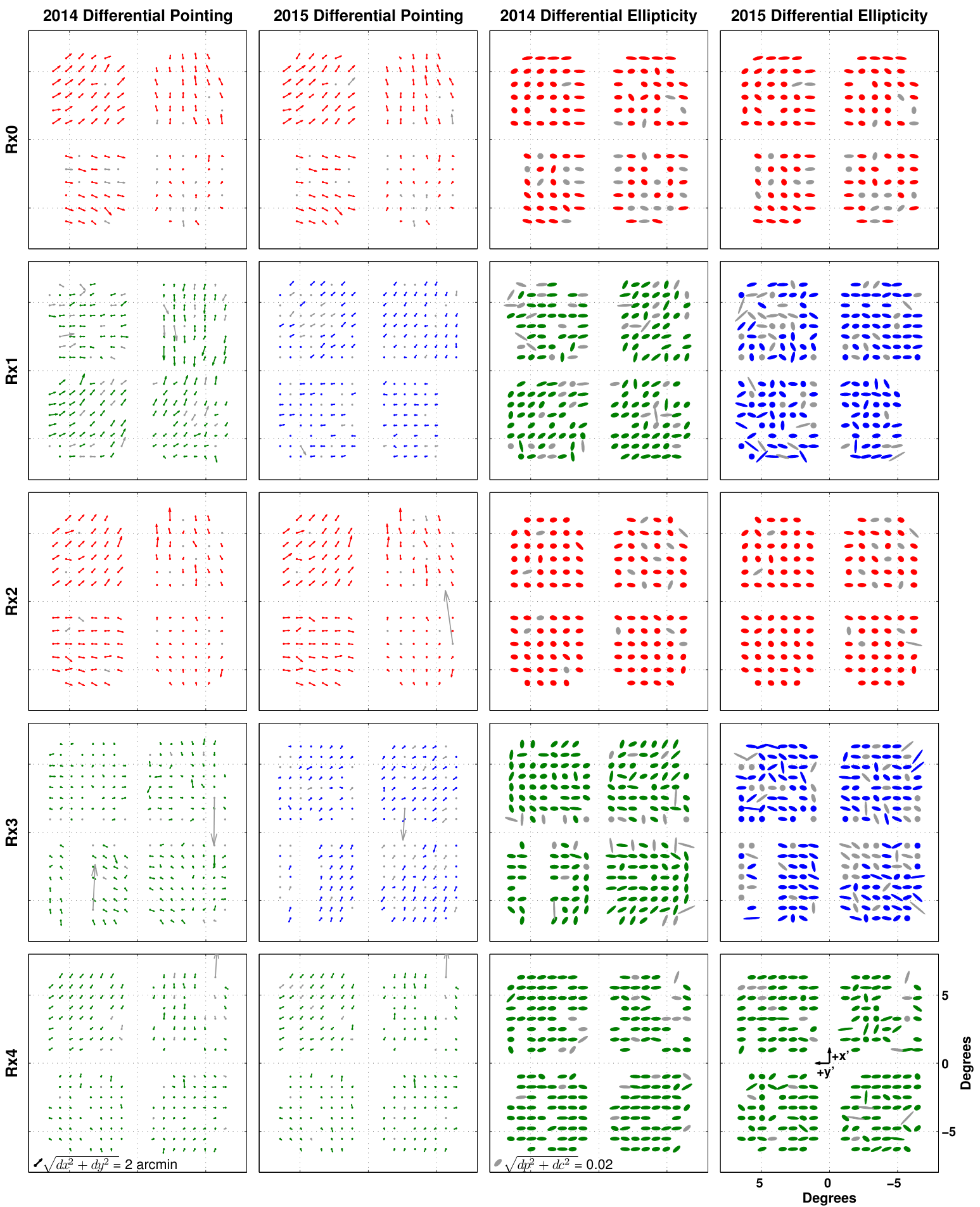
Figure 3 shows differential pointing and ellipticity for all Keck Array 2014 and 2015 receivers in focal plane layout. Differential pointing is usually the beam shape mismatch mode that causes the most leakage.55 5 While relative gain is also important, it is not measured in beam mapping because beam map normalization effectively deprojects it. For CMB analysis, relative gain is corrected at the timestream level by normalizing by the response to a small change in atmospheric loading (“elevation nods”), and at the map level by deprojection. Several trends stand out: first, measurements are consistent between years in which the receiver did not change (e.g. Rx0 in 2014 and 2015). Second, the absolute magnitude is somewhat frequency-dependent—95 GHz receivers show larger offsets than both 150 and 220 GHz, which are similar to each other—but there is large variability. Finally, it is typical to have a coherent differential pointing direction across a detector tile. Significant effort at the design and fabrication stages has been spent in reducing this mode, resulting in tiles with factors of 2–4 lower differential pointing than earlier, BICEP2-era tiles (O’Brient et al. 2012). Differential ellipticity is similarly consistent from year to year and coherent within tiles; appears to dominate.
We have checked that the deprojection coefficients—which scale templates of the Planck temperature sky and its derivatives to best fit the CMB data—match measured beam parameters and exhibit scatter consistent with their noise. On-sky data confirm that the CMB maps and far-field beam maps measure the same dominant beam mismatch modes (BK-III).
It is the higher-order residuals, not captured by the above second-order expansion of the beam profile, which could contribute leakage to the final polarization maps. To move beyond differential Gaussians we require sensitive beam maps capable of capturing the potentially-complex higher-order difference beam morphology.
IV Composite Beam Maps and Beam Profiles
To fully assess the impact of beams in CMB analysis we use deep far-field measurements extending to several degrees away from the beam center. In this section we describe how the beam maps generated in Section II—hereafter denoted “component” maps—are combined to form high-fidelity “composite” maps. Using composite beam maps reduces noise and systematics in the beam measurement and allows us to measure the main beam at all azimuthal angles.
IV.1 Noise and Systematics in Beam Measurements
Typical noise levels in a single pair’s component beam maps (i.e. from one measurement made with the 45 cm chopper) would induce a bias on the prediction of leakage from mismatched beams equivalent to at 150 GHz even if the beams were perfectly matched66 6 Beam map noise is measured by taking the standard deviation of pixel values in a region of the map far away from the main beam and ground contamination (i.e. more than above the beam). For 150 GHz detectors measured with the 45 cm chopper, the typical rms noise level in pixels is 1/800 of the main beam amplitude. The bias on is estimated by generating Gaussian noise simulations with these amplitudes and running them through the beam map simulation pipeline. (see Section V.2). This bias and uncertainty can be reduced by combining maps from multiple measurements. The average pair has good maps per year (Section III), so assuming Gaussian noise and a systematic error-free measurement, we expect to measure leakage with an uncertainty of for a single pair in a given year after averaging. Similarly—since our estimate of leakage for the CMB map is made by coadding the predicted leakage maps from all pairs—if noise is uncorrelated across detectors, the uncertainty on the final leaked estimate scales down with the number of pairs. Therefore, if there is real structure in the higher-order difference beams at a level that could be important for CMB analysis, we fully expect the beam maps to measure it. Since the 45 cm chopper noise level already outperforms our requirements, the current 60 cm thermal chopper will be well below the requirement for the next generation of BICEP experiments.
The most prominent systematic in the beam map measurement is ground-fixed contamination, which leaks into the in-phase demodulated signal at a low level.77 7 This contamination arises when scanning across a change in temperature, such as from cold sky to the (relatively) warm South Pole Telescope. Part of that temperature change is interpreted by the deconvolution kernel as signal from the thermal chopper. Ground-fixed signal usually enters into the measurement at the dB level or lower. We conservatively choose to mask out all regions of the map with known ground-fixed structure. To measure the regions of the beam that were masked, the receiver is rotated about the boresight axis and another map is made.
Other potential systematics include curvature in the redirecting mirror, the finite distance of the source, and nonlinearity in the detector response at the relatively high loading conditions used in calibration measurements. Using the measured mirror curvature88 8 Using in situ photogrammetry we have constrained the mirror’s flatness to better than 1.5 mm across its surface. we find that the absolute beam shape experiences a very small change— changes by for the 220 GHz beams at —and the differential beam shapes will see even less distortion because both detectors in a pair reflect off the mirror nearly identically. Through simulation of the beam shape error expected for a measurement at 210 m instead of at infinity, we find that BICEP3 with a nominal far-field distance of 171 m experiences a deviation of at ; the effect will be smaller for all Keck Array bands. Finally, we constrain nonlinearity on the high-loading aluminum transition sensor to be using load curves in which the detector bias voltage is ramped, providing an I-V characteristic.
Nonrepeatable contamination, i.e. non-Gaussian noise, is more worrisome and most often consists of single-sample glitches, which manifest as “hot spots” in the demodulated timestreams. A single glitch in the timestream can have an amplitude much larger than that of the main beam, resulting in a leakage prediction orders of magnitude larger than the true value even if the rest of the beam map were accurate.
For this reason we regard the differential beam maps as upper limits on the leakage from mismatched beams: they should capture all true leakage within the beam map radius, but could also contain non-Gaussian noise or measurement systematics that are difficult to quantify. Looking towards future results, we have demonstrated a reduction in beam map contamination through improved low-level deglitching and data quality cuts. These improvements will find application both in reanalysis of existing beam map data and in future datasets.
IV.2 Composite Beam Map Generation

Composite beam maps are generated by combining component maps that have passed data quality cuts and in which known, spatially-fixed contamination has been removed. We begin with the set of component maps from which beam statistics were calculated (Section III). We then apply a spatial mask: the ground ( below the source), the mast, and the South Pole Telescope are removed. Maps are centered on the common pair centroid, rotated to account for boresight angle, and peak-normalized. Finally the composite is made by assembling a stack of all good maps and taking a median in each spatial pixel. We take a median instead of a mean because occasionally high-amplitude artifacts escape the automated cuts. In current Keck Array maps, median-filtering results in demonstrably lower noise levels and fewer artifacts than mean-filtering. In future datasets we plan to improve low-level deglitching and spatial coverage to the point at which a mean may be taken.
Figure 4 shows sample composite beam maps and the component maps used to form them at the three Keck Array frequencies. The component maps have been masked for ground-fixed signal. Noise reduction and rejection of spurious contaminating signals are evident in the composites.
In principle it is best to use measurements that extend far away from the beam center to capture as much of the optical response as possible. We note, however, that in standard CMB observations the comoving forebaffle absorbs off-axis response at large angles (generally from the main beam). Since the forebaffles are removed to make room for hoisting the far-field flat mirror, response measured in the far-field beam maps at very large angles may not correspond to real beam pickup during CMB scans.99 9 In separate measurements, we use an amplified microwave source to measure far sidelobes. Comparing such maps made with and without the forebaffle, we see no perceptible difference in the main beam region. We expect any such difference to be extremely small, given the small amount of power intercepted (, see BK-IV) and the very efficient absorption of this power by the forebaffle. The composite maps also become noisier further away from the beam center because there are fewer hits per pixel as a result of the spatial masking. For the beam map simulation we use composites made out to from the beam center (Section V).
IV.3 Beam Profiles
To generate array-averaged beam profiles we coadd the composite maps over all detectors contributing to CMB data, inversely weighted by CMB-derived per-detector noise. Figure 5 shows the averaged radial profiles and the equivalent window functions. To remove the effect of the finite size of the source aperture, we divide by , where is the Bessel function of the first kind and is the angular diameter of the source as seen from the telescope. Typical detector-to-detector variations at are 2.6% (95 GHz), 2.2% (150 GHz), and 3.7% (220 GHz); the statistical uncertainty on individual beam profiles is small compared to this variation. We use these beam profiles in CMB analysis to smooth input maps for signal simulations and to smooth the Planck temperature sky and its derivatives, which serve as deprojection templates.
V Simulation of Temperature-to-Polarization Leakage
To estimate the leakage present in the BK15 maps we run “beam map simulations” with composite beam maps such as those presented in Section IV.1010 10 Although the term “simulation” is used, all inputs are based on real data: Planck maps, detector pointing, and on-sky beams measured in situ at South Pole. In this section we review how the simulations are generated and show the predicted leaked polarization maps and power spectra. The auto power spectra represent upper limits to the leakage in the BK15 maps due to mismatched beam shapes within polarization pairs. We then take the cross spectra of the beam map simulations with the real BK15 maps, which represent our best estimate of the leakage present in CMB data.
V.1 Simulation Methodology and Leakage Estimates
The standard BK15 pipeline is used to run beam map simulations. We inject leakage at the timestream level by convolving the Planck temperature sky with the per-detector beam maps and sampling from the resulting smoothed maps using real detector pointing data.1111 11 The detector-centered, locally-flat beam maps are scaled and rotated using the full spherical geometry appropriate for each detector’s pointing trajectory prior to convolution with a flat-sky projection of the Planck map. The Planck beam has been deconvolved from the temperature map. We intentionally set the Planck maps to zero so that any measured polarization is a result of leakage from mismatched beams. The timestreams are then processed into maps just as are the real data, including identical cuts and detector weighting. Deprojection of differential gain/pointing and subtraction of differential ellipticity are also applied1212 12 There is a small mismatch between the simulation timestreams (formed from flat-sky convolutions) and the deprojection templates (formed from curved healpix maps), but we have demonstrated that it corresponds to and is negligible; see BK-III for details. (see Section III). As in our standard -mode analysis, bandpowers are measured after applying a matrix-based purification that reduces leakage from partial sky coverage and filtering (Keck Array/BICEP2 Collaborations VII 2016) so that only the leakage modes relevant for our actual CMB maps are used. All beams contributing to the BK15 maps, including BICEP2 and Keck 2012–2013 (BICEP2/Keck Array Collaborations IV 2015), are accounted for in these results.
We assess the impact of a systematic contribution to a single-frequency spectrum with a quadratic estimator that is the equivalent level of the contamination. The estimator is
| (3) |
where are the systematic bandpowers predicted from the beam map simulation, is the bandpower covariance matrix from signal + noise simulations (“signal” refers to our fiducial lensed-CDM + dust skies and “noise” matches that of the BK15 maps), and are the bandpower expectation values for an signal. This effectively weights the systematic bandpowers by the ratio of the expected signal to the noise variance in each bin. For BICEP/Keck Array, most of the statistical power in the estimate comes from the first three bins (BICEP1 Collaboration 2014).
V.2 Simulation Results

Only the component of the pair difference beam remaining after deprojection (the “undeprojected residual”) is relevant for assessing the main beam leakage in the BK15 map. To illustrate typical difference beams, in Figure 6 we plot example composite maps for both and detectors in a pair, the pre-deprojection difference map, the difference map with differential pointing removed, and the final undeprojected residual. Amplitudes of features in typical undeprojected residual maps are of the main beam peak.
Far-field beam maps routinely identify features in individual detector pairs that contribute excess leakage. To illustrate, we show a 95 GHz beam that contains a large feature in the undeprojected residual, caused by a well-characterized anomalous interaction between the detector tile corrugations and the tile edge detectors. The impact on the undeprojected residuals and the subsequent remedy is discussed in more detail in Section V.3.
The maps of residual leakage predicted using the composite beam maps are shown in Figure 7. An estimate of the beam map noise is also shown, and discussed in more detail below. We expect all of the true leakage to be captured in these maps, but again emphasize that there is likely a nonnegligible contribution from systematics in the beam measurement.
While in general there is no expectation that undeprojected residuals should prefer or , it is not uncommon for the leakage to contaminate one over the other. For example, the 95 GHz tile corrugation feature shown in Figure 6 leaks primarily to modes because it is aligned with the detector polarization axes (the beam)—leakage aligned at would leak to (see BK-III for more details).
The central region of the 150 GHz map contains a band of lower leakage, which is due to the complex interaction of the rotational symmetry of undeprojected residuals (which determines whether they cancel under boresight rotation), their distribution across the focal plane (which determines whether they cancel when coadded with other detectors), and the combination of the many distinct receivers that contribute to the map.
The BB spectra corresponding to these maps are shown in Figure 8. We present both noise-debiased auto spectra and cross spectra of the beam map simulations with the BK15 maps. The interfrequency cross spectra, corresponding to leakage that correlates across frequencies, are consistent with zero within the uncertainties and are not plotted here.
The beam map auto spectra (black lines) represent upper limits to the single-frequency leakage since the beam measurement may contain low-level systematics. We estimate the noise contribution by forming a “beam map jacknife” for each detector pair. For each beam, we randomly divide the component maps into two halves and form two separate composite maps. The difference between these maps is effectively a jackknife in which the signal is removed and the noise remains (Figure 7 right column). This measure of noise bias has been subtracted from the beam map auto spectrum. The estimates for the upper limits and the jackknives are shown in Table 4 and indicate that the noise contribution to the beam maps is subdominant compared to the combination of true beam mismatch and potential systematics in the measurement.
The cross spectra with the BK15 maps (teal crosses; see BK-X Figures 7–9) offer an unbiased estimate of leakage in the real data and should be insensitive to systematics in the beam measurement; estimates are shown in Table 4. Uncertainties in the cross spectra arise from several sources: instrumental and atmospheric noise, the true-sky lensing and dust modes, and noise in the beam map measurement. To estimate the uncertainty from the CMB half of the cross spectrum, we use our ensemble of 499 -mode lensing, dust, and noise (i.e. instrumental and atmospheric) simulations—see BK15 for more details. Using the single beam map simulation, we take the 499 cross spectra:
The variance of these cross spectra constitute the error bars in Figure 8, which are propagated through to uncertainties on the estimates (“Cross spectrum ” in Table 4). Since the beam map jackknife is negligible compared to this, uncertainty in the beam measurement is not included here.
| 95 GHz | 150 GHz | 220 GHz | |
|---|---|---|---|
| Upper Limit | |||
| Beam Map Jackknife | |||
| BK15 Cross Spectrum | |||
| Cross Spectrum |
V.3 Discussion
Tracing leakage from input beam maps to the final spectra provides insight into detector and optics fabrication effects that can be improved. For example, the large tile corrugation feature in the 95 GHz pixels (Figure 6) impacted about half of the detectors contributing to the map, and has been corrected in focal planes produced subsequently. The contribution of these detectors is extremely anomalous; our present 95 GHz results are over an order of magnitude larger than what they would be if the tile edge detectors were excluded (Karkare 2017).
Do the beam map simulations correlate with the real BK15 maps and detect leakage? At 95 and 150 GHz the cross spectra are generally positive and follow the auto spectra, but are a factor of lower. Given the error estimates— at 95 GHz and at 150 GHz—there is only tentative evidence for leakage in the real BK15 maps. The suppression of the cross with respect to the auto could indicate nonnegligible systematics in the beam map measurement, which would bias the upper limits high and fail to correlate with the real maps.
At 220 GHz there is more power in the real map (due to dust and higher noise levels; see BK-X), so the large fluctuations in the cross with real are not unexpected. It seems likely that the uncertainties are underestimated. While Table 4 indicates that the beam map statistical errors are a factor of 20 lower than the auto spectrum, it is possible that systematics in the beam map measurement contribute extra variance to the cross spectrum that is not captured in the jackknife estimate. For example, visual inspection of the beam maps shows that contamination from the ground and mast is much more prominent at 220 GHz than at 95 and 150 GHz, and may leak into pixels that are not spatially masked at a level below the noise of an individual map. Future work with more rigorous masking of fixed structure is likely to improve the quality of these maps. Given these caveats, the recovered should not be taken as evidence for leakage.
Taken together, the beam map simulations do not definitively detect leakage in cross-correlation with CMB. The 95 and 150 GHz maps show a excess which cannot exclude zero leakage. At 220 GHz the cross spectra fluctuate enough to suggest underestimated error bars, and no real indication of leakage within the uncertainty. We also note that because this frequency mostly measures dust emission, the sensitivity of recovery on its leakage is weak.
VI The Effect of Undeprojected Residuals on Parameter Recovery
The BICEP/Keck likelihood analysis uses maps at several frequencies to separate the CMB from foregrounds (see BK-X). The single-frequency estimators of leakage that we used in Section V are therefore not representative of the effective bias on that we may incur from this potential additive systematic once all spectra are accounted for. In this Section, we discuss several methods of dealing with systematics in analysis. Using the auto and cross spectra presented in Section V.2, we then simulate the potential effect of this leakage on recovery in the multicomponent likelihood analysis.
VI.1 Treating Systematics in Analysis
How we deal with systematics in analysis depends on the uncertainty in the systematic’s form. In the case of a well-characterized effect—i.e. in which the specific morphology of the leakage is known—we would simply subtract the leaked signal in the time or map domain.
If we had intermediate knowledge of the systematic—such as a well-characterized amplitude, but not specific form—we would calculate the leakage bandpowers and debias them from the real data. The uncertainty on the debias would need to be included, e.g. by inflating the bandpower covariance matrix.
Finally, if there were substantial uncertainty on both the form and amplitude—e.g. if the uncertainty on the systematic is comparable to the estimated level of the systematic itself—there is little argument for debiasing. In this case, we would run simulations to determine whether the likely amplitude is small compared the the experiment’s statistical uncertainty.
In Section V.3 we analyzed the cross spectra of the beam map simulations with the BK15 maps and found that the uncertainty on the predicted leakage is comparable to its amplitude (Table 4). Since we cannot verify the amplitude of this leakage in the real CMB maps at high confidence, we will show that when propagated through the multicomponent likelihood, this potential systematic is subdominant compared to the statistical errors.
VI.2 Simulating Leakage in the Multicomponent Analysis
Here we use simulations to find the bias on that the BK15 likelihood analysis would incur if leakage levels consistent with either the beam map auto spectra or the cross spectra between beam maps and CMB data existed in the real maps. We also test the possibility of fitting for and marginalizing over a leakage template.
The BK15 likelihood analysis uses all available auto and cross spectra between the BK15 95, 150, and 220 GHz maps and external Planck and WMAP maps to generate a joint likelihood of the data for a particular parametric model. For details on the likelihood implementation see BICEP2/Keck Array/Planck Collaborations 2015; Keck Array/BICEP2 Collaborations VI 2016; Keck Array/BICEP2 Collaborations X 2018.
To gauge the impact of leakage on recovery, we analyze the shift in the maximum-likelihood value () for sets of 499 simulated bandpowers that have had bias added corresponding to one of the leakage estimates. Note that we calculate for the peak of the multi-dimensional likelihood, not the peak of the marginalized posterior pdf; we find that this provides a more direct view of biases in the analysis and is easily extended to non-physical negative values of to avoid truncation of the distribution. Histograms of from simulations are used as validation in the baseline BK15 analysis (Figure 20 of BK-X), and we use the standard deviation of that distribution as a measure of experimental sensitivity, for BK15.
For each leakage scenario, we look at the distribution of realization-by-realization shifts in relative to a baseline that does not include leakage in the simulation bandpowers and does not consider leakage parameters in likelihood analysis (this baseline analysis exactly corresponds to Figure 20 of BK-X). For the “upper limit” scenarios we report the median of the 499 shifts, while for the others we report the 16th, 50th, and 84th percentiles to reflect potentially-asymmetric distributions. Details of each scenario are listed below; the results are illustrated in Figure 9.
- •
Two “upper limit-driven” scenarios: We inject leakage consistent with the beam map simulation auto spectra (black lines in Figure 8), and ignore it in the likelihood analysis. Recall that the auto spectra are upper limits since they may be biased by systematics in the beam measurement. If we simply add the full beam map auto spectra (Figure 8 black curves) to the simulations—a situation we consider extremely unlikely—we find a median bias of (Scenario 1). To better reflect our belief in the auto spectra as 95% upper limits, in a second scenario we inject leakage with the same shape as the auto spectra, but with variable amplitude drawn from a Gaussian distribution centered at zero with of the nominal amplitude, and truncated at zero so only positive leakage can be added. The median bias is (Scenario 2).
- •
A “CMB data-driven” scenario: We inject leakage consistent with the cross spectra between the beam map simulations and the BK15 maps, and ignore it in likelihood analysis. Specifically, each realization is biased by a leakage contribution that is randomly drawn from the Figure 8 teal points and error bars. This is an attempt to model the leakage that appears to actually exist in the maps, albeit at marginal significance. The recovered bias is (Scenario 3).
- •
Three “recovery” scenarios: Using knowledge of the leakage from beam map simulations, we attempt to marginalize over it in the likelihood. For each frequency we add a new parameter to the likelihood analysis, which scales the leakage bias contribution to the bandpowers. For example, the parameter represents zero leakage in the 95 GHz map, while indicates leakage equal to that shown in the left panel of Figure 8. For this analysis, we must select one of the two leakage estimates to use as a template—either the beam map simulation auto spectrum or the beam map simulation cross spectrum with BK15 maps. We use a flat prior on in the range of . If the template used in the analysis matches the leakage added to the simulations, the resulting bias on is small: (Scenario 4). If the wrong template is used (e.g. inject the beam map/CMB cross spectrum, but fit for the beam map auto spectrum), we incur a negative bias: (Scenario 5). Finally, if no leakage is injected but we attempt to fit for it, we still find negative bias with (Scenario 6).
We take the “CMB data-driven” Scenario 3, , as our best estimate of the bias on from leakage. Figure 9 illustrates that in all cases the bias is subdominant compared to the BK15 statistical error, . Quadrature addition of the worst-case upper limit bias inflates by 8%.
In the standard COSMOMC analysis of e.g. BK15, physical priors are imposed. If we introduce a component that i) is partially degenerate with the signal of interest (), ii) is not clearly detected at the available noise level, and iii) has a positive-only prior applied, tends to be biased downwards. Since we do not clearly detect leakage in the current data, we decide not to marginalize over the parameters in the constraint analysis at this time. This is analogous to the treatment of the dust decorrelation parameter as discussed in Appendix F of BK15. We will continuously review this situation going forward.
VII Conclusions
In this paper we presented far-field optical characterization of Keck Array detectors at 95, 150, and 220 GHz contributing to the BK15 dataset. From an extensive far-field beam mapping campaign we measured differential Gaussian parameters with high precision, which are repeatable from year to year. For each detector we formed deep composite maps covering all azimuthal angles, and from them generated array-averaged beam profiles.
The composite beam maps were then used to predict the residual main beam leakage expected in the BK15 polarization maps after deprojection of the lowest-order beam mismatch modes. From an auto spectrum analysis of beam map simulations, noting that there may exist contributions from low-level systematics in the beam measurement, we presented upper limits to the leakage. Cross spectra between the beam map simulations and the BK15 CMB maps offer tentative evidence for leakage, but the uncertainties are large enough that zero leakage cannot be excluded.
We have run simulations using the BK15 multicomponent likelihood analysis to test the effect of undeprojected leakage on recovery. When leakage consistent with the cross spectra between beam map simulations and real CMB maps is added, the bias is . It is possible to marginalize over this contribution in the multicomponent analysis, but this admits the possibility of a small negative bias if the wrong template is used with physical priors. Because the leakage is not clearly detected in the CMB data, we do not marginalize over it in the current constraint on . All of the biases presented are small compared to the BK15 statistical uncertainty .
BICEP’s sensitivity to will continue to steadily improve: with data taken through the 2017 season we expect , and with the BICEP Array experiment under construction we anticipate within five years (Hui et al. 2018). Constraints on beam systematics will need to similarly tighten. Future effort will focus on three aspects of the problem: the intrinsic leakage level, the measurement thereof, and treatment in analysis.
High-fidelity beam maps point to features in individual beams that contribute significant leakage, which can then be remedied in hardware. Such feedback has been critical to ensuring that leakage is reduced in later generations of receivers. For example, the 95 GHz difference beam shown in Figure 6 highlighted an anomalous interaction between the tile corrugations and edge detectors. Compared to detectors that were not affected, the tile edge detectors drove up the estimated leakage for the BK15 results by over an order of magnitude. We corrected this effect in focal planes produced subsequently, and expect that this feedback cycle will continue.
Looking beyond the BK15 result, we have already improved the beam map reduction compared to the maps presented in this paper: non-Gaussian noise has been significantly reduced through more optimal low-level deglitching and demodulation. Re-reduction of existing data will produce cleaner maps and allow us to mean-filter the component maps when generating the composites. In future beam mapping campaigns we also plan to modify the raster scan strategy to produce robust noise estimates, e.g. by using out-and-back scans at the same elevation to form a “scan direction” jackknife. Maps generated from these data will be used to generate beam map noise realizations without dividing the composite maps into two halves. Their enhanced statistical properties will facilitate comparison of leakage to CMB data.
While in this paper we have shown a basic attempt to detect leakage by cross-correlating the final coadded leakage and real CMB maps (in which much of the leakage has cancelled), this comparison can be improved. In our next results we plan to form cross spectra that detect the predicted leakage at high significance. We will isolate high-leakage detector subsets or form combinations of on-sky data that are expected to enhance the leakage (e.g. boresight angles that do not cancel) in particular sub-maps compared to the full dataset. Given these higher-confidence estimators of leakage in the CMB maps, we will explore several options to remove the effect. If the number of high-leakage detectors is small, excluding or de-weighting them will dramatically improve systematic control. With improved statistical properties of the beam maps, debiasing as discussed in Section VI.1 would also be reasonable. Finally, we can further reduce residuals by deprojecting additional modes of this leakage for each detector pair. This can be done using modes drawn from bases independent of the beam maps, by using the beam maps to directly predict the template of each pair’s undeprojected residual, or by using these maps to guide definition of a small subset of modes to be deprojected.
References
- Bennett et al. (2013) Bennett, C. L., Larson, D., Weiland, J. L., et al. 2013, Astrophys. J. Suppl. Ser., 208, 20
- Buder et al. (2014) Buder, I., Ade, P. A. R., Ahmed, Z., et al. 2014, in Proc. Soc. Photo-Opt. Instrum. Eng., Vol. 9153, Millimeter, Submillimeter, and Far-Infrared Detectors and Instrumentation for Astronomy VII, 915312
- CMB-S4 Science Book (2016) CMB-S4 Science Book. 2016, ArXiv e-prints, arXiv:1610.02743
- BICEP1 Collaboration (2014) BICEP1 Collaboration. 2014, Astrophys. J., 783, 67
- BICEP2 Collaboration II (2014) BICEP2 Collaboration II. 2014, Astrophys. J., 792, 62
- BICEP2 Collaboration III (2015) BICEP2 Collaboration III. 2015, Astrophys. J., 814, 110
- BICEP2/Keck Array/Planck Collaborations (2015) BICEP2/Keck Array/Planck Collaborations. 2015, Physical Review Letters, 114, 101301
- BICEP2/Keck Array Collaborations IV (2015) BICEP2/Keck Array Collaborations IV. 2015, Astrophys. J., 806, 206
- Keck Array/BICEP2 Collaborations VI (2016) Keck Array/BICEP2 Collaborations VI. 2016, Physical Review Letters, 116, 031302
- Keck Array/BICEP2 Collaborations VII (2016) Keck Array/BICEP2 Collaborations VII. 2016, Astrophys. J., 825, 66
- Keck Array/BICEP2 Collaborations VIII (2016) Keck Array/BICEP2 Collaborations VIII. 2016, Astrophys. J., 833, 228
- Keck Array/BICEP2 Collaborations X (2018) Keck Array/BICEP2 Collaborations X. 2018, Physical Review Letters, 121, 221301
- Conklin (1969) Conklin, E. K. 1969, Nature, 222, 971
- Hanson et al. (2013) Hanson, D., Hoover, S., Crites, A., et al. 2013, Physical Review Letters, 111, 141301
- Hu et al. (2003) Hu, W., Hedman, M. M., & Zaldarriaga, M. 2003, Phys. Rev. D, 67, 043004
- Hui et al. (2018) Hui, H., Ade, P. A. R., Ahmed, Z., et al. 2018, in Society of Photo-Optical Instrumentation Engineers (SPIE) Conference Series, Vol. 10708, Millimeter, Submillimeter, and Far-Infrared Detectors and Instrumentation for Astronomy IX, 1070807
- Kamionkowski & Kovetz (2016) Kamionkowski, M., & Kovetz, E. D. 2016, Ann. Rev. Astron. Astrophys., 54, 227
- Karkare (2017) Karkare, K. S. 2017, PhD thesis, Harvard University
- Karkare et al. (2016) Karkare, K. S., Ade, P. A. R., Ahmed, Z., et al. 2016, in Proc. Soc. Photo-Opt. Instrum. Eng., Vol. 9914, Millimeter, Submillimeter, and Far-Infrared Detectors and Instrumentation for Astronomy VIII, 991430
- Keisler et al. (2015) Keisler, R., Hoover, S., Harrington, N., et al. 2015, Astrophys. J., 807, 151
- Kovac et al. (2002) Kovac, J. M., Leitch, E. M., Pryke, C., et al. 2002, Nature, 420, 772
- Louis et al. (2017) Louis, T., Grace, E., Hasselfield, M., et al. 2017, Journal of Cosmology and Astro-Particle Physics, 2017, 031
- O’Brient et al. (2012) O’Brient, R., Ade, P. A. R., Ahmed, Z., et al. 2012, in Proc. Soc. Photo-Opt. Instrum. Eng., Vol. 8452, Millimeter, Submillimeter, and Far-Infrared Detectors and Instrumentation for Astronomy VI, 84521G
- Penzias & Wilson (1965) Penzias, A. A., & Wilson, R. W. 1965, Astrophys. J., 142, 419
- Planck Collaboration et al. (2016) Planck Collaboration, Adam, R., Ade, P. A. R., et al. 2016, Astron. Astrophys., 594, A1
- Planck Collaboration et al. (2018) Planck Collaboration, Aghanim, N., Akrami, Y., et al. 2018, arXiv e-prints, arXiv:1807.06210
- Polarbear Collaboration (2014) Polarbear Collaboration. 2014, Astrophys. J., 794, 171
- Smoot et al. (1992) Smoot, G. F., Bennett, C. L., Kogut, A., et al. 1992, Astrophys. J. Lett., 396, L1
- Wong (2014) Wong, C. L. 2014, PhD thesis, Harvard University