Abstract

This thesis describes our ongoing work on Contrastive Predictive Coding (CPC) features for speaker verification. CPC is a recently proposed representation learning framework based on predictive coding and noise contrastive estimation. We focus on incorporating CPC features into the standard automatic speaker verification systems, and we present our methods, experiments, and analysis. This thesis also details necessary background knowledge in past and recent work on automatic speaker verification systems, conventional speech features, and the motivation and techniques behind CPC.

Acknowledgments

I have the privilege to be advised by one of the best in the field of speech processing and surrounded by talented and motivated individuals who encourages me to make strides for the speech community. I want to give my sincere gratitude to my advisor at JHU, Professor Najim Dehak, who introduced me to speech processing and pushed me to become better every day. There were times that I could not make good progress and felt like giving up, and it was Najim who supported me through those difficult moments. I could never forget the trust Najim has given to me and he is the best advisor I can ask for as an undergraduate. Thanks to Dr. Jesús Villalba, who has infinite patience for me in the past two years. I came in to the field with little knowledge in machine learning and coding, and it was Jesús who guided me step by step and taught me to be persistent in research. Thanks to Professor Simon King, who hosted me at University of Edinburgh and gave me the resources, guidance, and research environment to work on anti-spoofing. I have the best summer ever at Edinburgh without a doubt. Thanks to Professor Hynek Hermansky, who advised me the importance of the basics and scrutiny of conducting good research. Thansk to Professor Korin Richmond, Professor Junichi Jamagishi, and Professor Alberto Abad, who patiently answered several questions I have on anti-spoofing during the several meetings we had. I would also like to thank Laure moro, for the Parkinson’s disease project and his help on improving my presentation skills, Phani Nidadavolu, for the bandwidth extension project and the good practices he taught me in conducting experiments, and Nanxin Chen, for helping me to learn coding, debug, discover sources for new research paper, and inspiring me to do creative work.

I would like to extend my gratitude to other members in the CLSP group at JHU and the CSTR group at University of Edinburgh, especially Professor Daniel Povey, Professor Shinji Watanabe, Professor Alan Yuille, Professor Colin Wilson, Professor Mounya Elhilali, Paola Garcia-Perera, Dimitra Emmanouilidou, Debmalya Chakrabarty, Arun Nair, Matthew Wiesner, David Synder, Lucas Ondel, Aswin Subramanian, Ruizhi Li, ChuCheng Lin, Raghavendra Reddy, JaeJin Cho, Saurabh Bhati, Peter Frederiksen, Saurabh Kataria, Xutai Ma, Xiaofei Wang, Kelly Marchisio, Sray Chen, Cassia Valentini, Catherine Lai, Joanna Równicka, Julie-Anne Meaney, Mark Sinclair, Felipe Espic, and Pacco.

I met a lot of brilliant people during college. Thanks to William Zhang, James Shamul, Justin Chua, Bijan Varjavand, Aurik Sarker, Harrison Nguyen, Eric Tsai, Kiki Chang, Vladimir Postnikov, Esther Tien, William Shyr, Jeff Peng, Kevin Chen, Kevin Ma, Chris Hong, Chin-Fu Liu, Ray Cheng, Tom Shen, Max Novick, Adriana Donis, Jillian Ho, Richard Oh, Alejandro Contreras, Cindy Yuan, Allen Ren, Linh Tran, Charlie Wang, Weiwei Lai, Michael Chan, and Emily Sun, for their love and support. Their kindness and presence have made all the differences in my life. I want to give special thanks to Daniel Hsu, who took good care of me when I was suffering from a herniated disc and sciatica, and for being an awesome roommate and friend. Finally, I want to thank my family members in Taiwan for supporting me emotionally and financially. I am especially grateful for my mom, who has always encouraged me to venture to a bigger world and do greater things.

intro_speaker_chapter/intro_chapter

Chapter 1 Conventional Speech Features

1.1 Introduction

The Feature Processing step in extracts low-level feature descriptors from raw waveform, and several earlier work showed that Fourier analysis based transforms can effectively capture information of speech signals. Conventional low-level speech features include Log-spectrogram, Log-Filterbank, Mel-Frequency Cepstral Coefficients (MFCC), and Peceptual Linera Predictive (PLP) Analysis. DNN-based speech recognition systems [hinton2012deep], GMM-UBM systems [reynolds2000speaker] and i-vectors systems [dehak2011front] are based on MFCC; x-vectors systems [snyder2018x] and LDE [cai2018exploring] are based on Log-Filterbank; Attentive Filtering Network [lai2018attentive] is based on Log-Spectrogram. We established our baseline on MFCC, and this chapter will introduce MFCC and the MFCC configuration used in our experiments in Chapter 3.

1.2 Mel-Frequency Cepstral Coefficients (MFCC)

MFCC is one of the most standard and common low-level feature in automatic speaker recognition systems. The procedure of MFCC extraction is followed:

1.

Take Short-Term Fourier Transform (STFT) on the waveform. This step will give us a Spectrogram.
2.

Apply Mel-scale Filters. This step will give us a Filterbank.
3.

Take the logarithm on the powers in all Mel-bins. Logarithm is taken also for Log-Spectrogram and Log-Filterbank.
4.

Apply Discrete Consine Transform (DCT), and keep several cepstral coefficients. This step decorrelates and reduces the dimensionality.

A visual comparison of Log-Spectrogram, Log-Filterbank, and MFCC is 1.1. We can see that there are more structures in Log-Spectrogram and Log-Filterbank, and MFCC has less dimensions than the former two.

Figure 1.1: An Visual Comparison of (top) Log-Spectrogram, (middle) Log-Filterbank, and (bottom) MFCC.

1.3 MFCC Details

Our experiments (see Chapter 3 for more details) are conducted on the LibriSpeech Corpus [panayotov2015librispeech], in which speech utterances are recorded in 16k Hz. We used the standard 25 ms frame-length and 10 ms frame-shift for STFT computation, 40 Mel filters, and took 24 cepstral coefficients after DCT. The first and second order derivatives (deltas and double-deltas) are computed during UBM training. Details of our MFCC configuration is in Table 1.1.

MFCC Details
Sampling Frequency	16000 Hz
Frame Length for STFT	25 ms
Frame Shift for STFT	10 ms
High Frequency Cutoff for Mel Bins	7600 Hz
Low Frequency Cutoff for Mel Bins	20 Hz
Number of Mel Bins	40
Number of Cepstral Coefficients after DCT	24

Table 1.1: Our MFCC Configuration. The configuration is mostly based on the Kaldi toolkit [povey2011kaldi].

Chapter 2 Contrastive Predictive Coding

2.1 Introduction

Predictive coding is a well-motivated and developed research area in neuroscience. The central idea of predictive coding is that the current and past states of a system contain relevant information of its future states. On the other hand, one long-standing research question in speech processing has been to extract global information from noisy speech recordings. In speech recognition, this can be related to as retrieving phone labels from the recordings. In speaker recognition, the same research question could be framed as sentiment analysis of the recordings. Could we harness the concept of predictive coding to design a model which extracts representations that are invariant to noise? Contrastive Predictive Coding (CPC) connects the idea of predictive coding and representation learning. This Chapter will give a background overview of predictive coding in neuroscience 2.2, a background of CPC 2.3 and CPC models 2.3. Lastly, the application of CPC for speaker verification is presented 2.5.

2.2 Predictive Coding in Neuroscience

In a famous study by [hubel1968receptive], the visual Receptive Field (RF) in the monkey striate cortex is studied. Macaque monkey is presented with line stimuli of different orientations while RF responses in the striate cortex are recorded. The experiment showed that cells responded optimally (with high firing rates) to particular line orientations, illustrated in Figure 2.1. The interesting question to ask here is: why don’t neurons always respond in proportion to the stimulus magnitude?

Figure 2.1: RF responses to line stimuli Illustration of the RF firing responses to the same line segment but different line orientations from a cell in the monkey striate cortex [hubel1968receptive]

Predictive coding is one prominent theory that aims to provide a possible explanation. Predictive coding states that human brain can be modeled by a framework that is constantly generating hypotheses and fixing its internal states through an error feedback loop. Since neighboring neurons are likely to be correlated, predictive coding implies that the RF response of a neuron can be predicted by those RF responses of its surroundings, and therefore a strong stimulus does not always correspond to a strong RF response. The first hierarchical model with several levels of predictive coding is proposed for visual processing in [rao1999predictive]. Each level receives a prediction from the previous level and calculates the residual error between prediction and the reality. To achieve efficient coding, only the residual error is propagated forward to the next level, while the next prediction for the current level is made, illustrated in Figure 2.2.

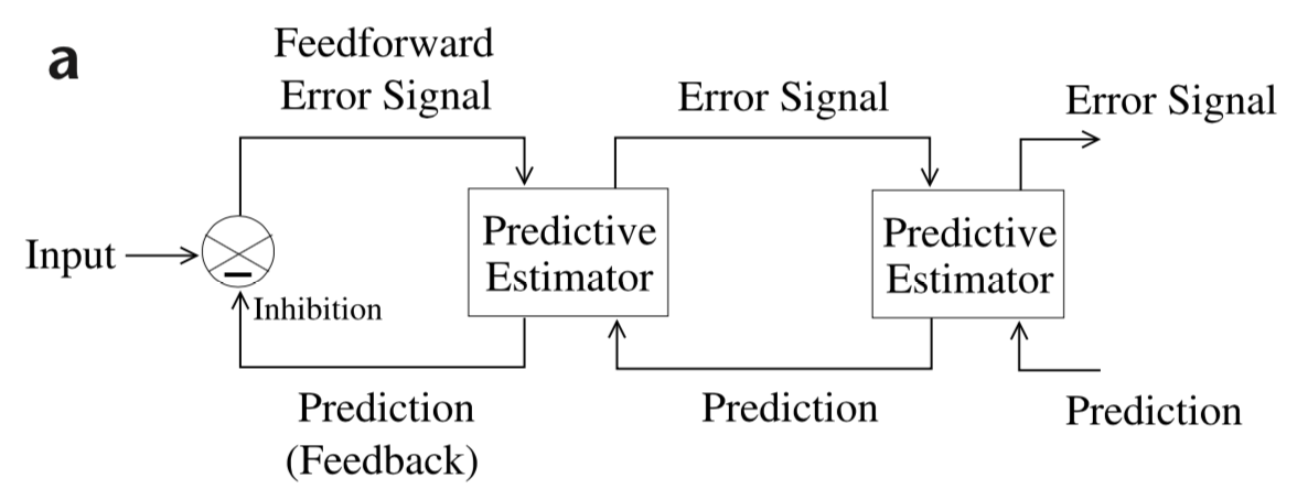
Figure 2.2: Hierarchical model of predictive coding Illustration of how residual error is propagated and how prediction is made in the hierarchical model in [rao1999predictive]

The study of [rao1999predictive] suggested the importance of feedback connection in addition to feedforward information transmission for visual processing. However, the key insight of how predictive coding is connected to representation learning is that by learning to predict, the model should implicitly retain properties or structures of the input.

2.3 Contrastive Predictive Coding (CPC)

2.3.1 Connection to Predictive Coding

Contrastive Predictive Coding (CPC) is proposed in [oord2018representation] as a new unsupervised representation learning framework. One challenging aspect of representation learning within high dimensional signal is noise. The primary goal of CPC is to extract high-level representation, or the slow-varying features [wiskott2002slow], from a sensory signal full of low-level noises. On the other hand, predictive coding retains properties or structures of the input 2.2. By predicting the future, the model has to infer global properties or structures from the past, and therefore has to separate global information from noises. One example is TV show series. After watching several episodes of a TV series, most people could generally predict some plots in the next few episodes. But only a few who know the entire series and its history very well can make plot predictions beyond five episodes. These few people has "mastered" the TV series such that they can tell the important plot development from those that are minor in comparison. CPC leverage this idea and therefore could be powerful for separating high-level representation from noises.

However, how do we quantify high-level representation and monitor how well the model is learning? To quantify high-level representation, CPC calculates the mutual information $I(x;C)$ between the sensory signal $x$ and global information $C$ . Let us refer back to the TV series example. The correct prediction of the plots in future episodes are often hidden as several key points in previous episodes. If we put it in terms of mutual information, the sensory signal $x$ is the future episode plots, and global information $C$ is the several key points, such as an important plot twist or character development. 2.3.2 gives a background of mutual information theory.

What metric should we use to train the predictive coding model? Figure 2.2 is the original hierarchical model of predictive coding proposed for visual processing, and from the figure we can see that the residual error is calculated during the feedforward pass. An straightforward implementation of residual error could be the L1 loss 2.3.1 or Mean Squared Error (MSE) 2.3.1 between prediction $D(H)$ and actual value $A$ , where $H$ is some learnable latent representation and $D$ is a mapping from the latent space to input space. In fact, this implementation can be dated back to the 1960s where MSE is used for training the predictive coding model for speech coding [atal1970adaptive]. Predictive Coding Network, another predictive coding based unsupervised learning framework, is trained with L1 loss [lotter2016deep]. However, either L1 loss or MSE loss requires a mapping function, namely a decoder $D$ , that computes $p(x\mid C)$ . In our TV series example, $p(x\mid C)$ is saying, "tell me all the details $x$ of future plots given the several key points $C$ . Intuitively, this is a hard task and unnecessary for our purpose since we are interested in high-level representations. To get around this issue, CPC models the mutual information directly with the noise contrastive estimation technique, which is introduced in 2.3.3.

\displaystyle L1=\sum_{i=1}^{N}(D(h_{i})-a_{i})^{2}

(2.1)

.

\displaystyle MSE=\sum_{i=1}^{N}\mid D(h_{i})-a_{i}\mid.

(2.2)

Figure 2.3: Predictive Coding Network (PredNet) Illustration of information flow in PredNet, which is trained with the L1 loss between

\hat{A_{l+1}}

and

A_{l+1}

. [lotter2016deep]

2.3.2 Mutual Information

Mutual information denotes the amount of information shared between the two variables. Given two random variable $X$ and $Y$ , mutual information $I(X;Y)$ is defined as,

\displaystyle I(X;Y)=H(X)-H(X\mid Y),

(2.3)

where $H(X)$ is the entropy of $X$ and $H(X\mid Y)$ is the conditional entropy of $Y$ given $X$ . $H(X)$ is defined as,

\displaystyle H(X)=-\sum_{i=1}^{n}P(X=x_{i})\log{P(X=x_{i})},

(2.4)

and $H(X\mid Y)$ is defined as,

\displaystyle H(X\mid Y)=-\sum_{i=1}^{n}P(X=x_{i}\mid Y)\log{P(X=x_{i}\mid Y)}.

(2.5)

With the above definitions, we can subsequently show the following:

\displaystyle I(X;Y)=\sum_{i=1}^{n}\sum_{j=1}^{m}p(x_{i},y_{j})\log{\frac{p(x_{i}\mid y_{j})}{p(x_{i})}}

(2.6)

Proof.

First we expand 2.3.2 as:

$\displaystyle H(X\mid Y)$	$\displaystyle=-\sum_{i=1}^{n}P(X=x_{i}\mid Y)\log{P(X=x_{i}\mid Y)}$	(2.7)
	$\displaystyle=-\sum_{i=1}^{n}\sum_{j=1}^{m}P(X=x_{i}\mid Y=y_{j})P(Y=y_{j})\log{P(X=x_{i}\mid Y=y_{j})}$	(2.8)
	$\displaystyle=-\sum_{i=1}^{n}\sum_{j=1}^{m}p(x_{i}\mid y_{j})p(y_{j})\log{p(x_{i}\mid y_{j})}$	(2.9)

Then by substitution and Baye’s rule,

$\displaystyle I(X;Y)$	$\displaystyle=H(X)-H(X\mid Y)$	(2.10)
	$\displaystyle=-\sum_{i=1}^{n}p(x_{i})\log{p(x_{i})}+\sum_{i=1}^{n}\sum_{j=1}^{m}p(x_{i}\mid y_{j})p(y_{j})\log{p(x_{i}\mid y_{j})}$	(2.11)
	$\displaystyle=-\sum_{i=1}^{n}\sum_{j=1}^{m}p(x_{i},y_{j})\log{p(x_{i})}+\sum_{i=1}^{n}\sum_{j=1}^{m}p(x_{i},y_{j})\log{\frac{p(x_{i},y_{j})}{p(y_{j})}}$	(2.12)
	$\displaystyle=-\sum_{i=1}^{n}\sum_{j=1}^{m}p(x_{i},y_{j})\log{\frac{p(x_{i})p(y_{j})}{p(x_{i},y_{j})}}$	(2.13)
	$\displaystyle=\sum_{i=1}^{n}\sum_{j=1}^{m}p(x_{i},y_{j})\log{\frac{p(x_{i}\mid y_{j})}{p(x_{i})}}$	(2.14)

∎

We can also easily show that if $X$ and $Y$ are independent, their mutual information is zero:

Proof.

Given $X$ and $Y$ are independent, $P(X\mid Y)=P(X)$ . By definition, we can rewrite $H(X\mid Y)$ as:

$\displaystyle H(X\mid Y)$	$\displaystyle=-\sum_{i=1}^{n}P(X=x_{i}\mid Y)\log{P(X=x_{i}\mid Y)}$	(2.15)
	$\displaystyle=-\sum_{i=1}^{n}P(X=x_{i})\log{P(X=x_{i})}$	(2.16)
	$\displaystyle=H(X),$	(2.17)

and therefore, we have:

$\displaystyle I(X;Y)$	$\displaystyle=H(X)-H(X\mid Y)$	(2.18)
	$\displaystyle=H(X)-H(X)$	(2.19)
	$\displaystyle=0$	(2.20)

∎

In the context of representation learning, mutual information gives us a quantitative measure of how well a model learns the global information. Let us look back at the TV series example again. If a person only has limited memory and has successfully observed the key developments, denoted as $C_{1}$ , over the past episodes, those developments are likely to be highly relevant to the upcoming episodes, denoted as $X$ . We can say that their mutual information $I(X;C_{1})$ is high. Hoewver, given the limited amount of memory everyone has, if the person only remembered the minor plot developments, denoted as $C_{2}$ , the mutual information $I(X;C_{2})$ is most likely to be low.

2.3.3 Noise-Contrastive Estimation (NCE)

Noise-Contrastive Estimation (NCE) is an estimation technique for estimating the parameters of parametric density functions [gutmann2012noise]. Let us consider a set of observations $X=(\vec{x_{1}},\vec{x_{2}},\vec{x_{3}},...,\vec{x_{N}})$ , where $\vec{x_{i}}\in{\mathbb{R}}^{n}$ . In real world examples, $n$ is often of high dimension, and the goal of all machine learning models is to find, or give an accurate estimate of, the underlying data distribution, the probability density function (pdf) $P_{D}$ , from the observable set $X$ . NCE makes an assumption that $P_{D}$ comes from a parameterized family of functions:

\displaystyle P_{D}\in\{P_{M}(;\boldsymbol{\theta})\},

(2.21)

where $\boldsymbol{\theta}$ is a set of parameters. Put it another way, there exists some $\theta^{\star}$ such that the following is true,

\displaystyle P_{D}=P_{M}(;\theta^{\star}).

(2.22)

Now, let us denote any estimate of $\theta^{\star}$ as $\bar{\theta}$ . Then, the following must hold for any pdf $P_{M}(;\bar{\theta})$ :

\displaystyle P_{M}(;\bar{\theta})\geq 0

(2.23)

\displaystyle\int P_{M}(\vec{x};\bar{\theta})d\vec{x}=1

(2.24)

If these two constraints are satisfied for all $\theta\in\boldsymbol{\theta}$ , then we say $P_{D}$ is normalized; otherwise, $P_{D}$ is unnormalized. It is common for models to be unnormazlied, such as the Gibbs distribution. Let us further give these unnormalized parametric models a name, $P^{0}_{M}(;\alpha)$ . To normalize $P^{0}_{M}(;\alpha)$ , we would need to calculate the partition function $Z(\alpha)$ :

\displaystyle Z(\alpha)=\int P^{0}_{M}(\vec{x};\alpha)d\vec{x},

(2.25)

and $P^{0}_{M}(;\alpha)$ can be normalized by $\frac{P^{0}_{M}(;\alpha)}{Z(\alpha)}$ .

Everything so far is reasonable, except that in real word examples, $Z(\alpha)$ is certainly intractable for high-dimensional data (curse of dimensionality), and thus $P^{0}_{M}(;\alpha)$ is still unnormalized. One simple solution NCE proposed is, why not make $Z(\alpha)$ an additional parameter [gutmann2012noise]? Let us define the new pdf $P_{M}(;\vec{\theta})$ accordingly:

\displaystyle\ln P_{M}(;\vec{\theta}):=\ln P^{0}_{M}(;\alpha)+c,

(2.26)

where $c=\frac{1}{Z(\alpha)}$ , and $\vec{\theta}=(\alpha,c)$ . The estimate $\bar{\theta}=(\bar{\alpha},\bar{c})$ now is not subject to the two constraints above since $\bar{c}$ provides a scaling factor. The intuition here is that instead of calculating $Z(\alpha)$ to normalize $P^{0}_{M}(;\alpha)$ for all $\alpha$ , only $P^{0}_{M}(;\bar{\alpha})$ is normalized.

However, Maximum Likelihood Estimation only works for normalized pdf, and $P^{0}_{M}(;\alpha)$ is not normalized for all $\alpha$ . NCE is therefore proposed for estimating unnormalized parametric pdfs.

2.3.3.1 Density Estimation in a Supervised Setting

The goal of density estimation is to give an accurate description of the underlying probablistic density distribution of an observable data set $X$ with unknown density $P_{D}$ . The intuition of NCE is that by comparing $X$ against a known set $Y$ , which has a known density $P_{N}$ , we can get a good grasp of what $P_{D}$ looks like. Put it more concretely, by drawing samples from $Y=(\vec{y_{1}},\vec{y_{2}},\vec{y_{3}},...,\vec{y}_{T_{y}})$ with a known pdf $P_{N}$ , and samples from $X=(\vec{x_{1}},\vec{x_{2}},\vec{x_{3}},...,\vec{x}_{T_{x}})$ , we can estimate the density ratio $\frac{P_{D}}{P_{N}}$ . With $\frac{P_{D}}{P_{N}}$ and $P_{N}$ , we have the target density $P_{D}$ .

By classifying samples $X$ from noise $Y$ with a simple classifier, in this case logistic regression, we show NCE gets a estimate of the probability density ratio $\frac{P_{D}}{P_{N}}$ .

Let $X$ and $Y$ be two observable sets containing data $X=(\vec{x_{1}},\vec{x_{2}},\vec{x_{3}},...,\vec{x}_{T_{x}})$ , $Y=(\vec{y_{1}},\vec{y_{2}},\vec{y_{3}},...,\vec{y}_{T_{y}})$ , and let $U$ be $X\cup Y$ , $U=(\vec{u_{1}},\vec{u_{2}},\vec{u_{3}},...,\vec{u}_{T_{x}+T_{y}})$ . $X$ is drawn from an unknown pdf $P_{D}\in\{P_{M}(;\boldsymbol{\theta})\}$ , and $Y$ is drawn from a known pdf $P_{N}$ . Since $Y$ is not our target, it is commonly referred to as the "noise". We also assign each datapoint in $U$ a label $C_{t}$ : $C_{t}=1$ if $u_{t}\in X$ and $C_{t}=0$ if $u_{t}\in Y$ . From the above settings, the likelihood distributions are then:

\displaystyle P(\vec{u}\mid C=1)=P_{M}(\vec{u};\boldsymbol{\theta})

(2.27)

\displaystyle P(\vec{u}\mid C=0)=P_{N}(\vec{u})

(2.28)

The prior distributions are:

\displaystyle P(C=1)=\frac{T_{x}}{T_{x}+T_{y}}

(2.29)

\displaystyle P(C=0)=\frac{T_{y}}{T_{x}+T_{y}}

(2.30)

The probability of the data $P(\vec{u})$ is thus:

	$\displaystyle P(\vec{u})$	$\displaystyle=P(C=0)\times P(\vec{u}\mid C=0)+P(C=1)\times P(\vec{u}\mid C=1)$		(2.31)
		$\displaystyle=\frac{T_{y}}{T_{x}+T_{y}}\times P_{N}(\vec{u})+\frac{T_{x}}{T_{x}+T_{y}}\times P_{M}(\vec{u};\boldsymbol{\theta})$		(2.32)

With Baye’s rule, we can derive the posterior distributions of $P(C=1\mid\vec{u})$ and $P(C=0\mid\vec{u})$ :

$\displaystyle P(C=1\mid\vec{u})$	$\displaystyle=\frac{P(C=1)\times P(\vec{u}\mid C=1)}{P(\vec{u})}$	(2.33)
	$\displaystyle=\frac{\frac{T_{x}}{T_{x}+T_{y}}\times P_{M}(\vec{u};\boldsymbol{\theta})}{\frac{T_{y}}{T_{x}+T_{y}}\times P_{N}(\vec{u})+\frac{T_{x}}{T_{x}+T_{y}}\times P_{M}(\vec{u};\boldsymbol{\theta})}$	(2.34)
	$\displaystyle=\frac{P_{M}(\vec{u};\boldsymbol{\theta})}{P_{M}(\vec{u};\boldsymbol{\theta})+vP_{N}(\vec{u})}$	(2.35)

where

\displaystyle v=\frac{T_{y}}{T_{x}}.

(2.36)

Similarly, we can get

\displaystyle P(C=0\mid\vec{u})=\frac{vP_{N}(\vec{u})}{P_{M}(\vec{u};\boldsymbol{\theta})+vP_{N}(\vec{u})}

(2.37)

$P(C=1\mid\vec{u})$ can further be expressed as,

	$\displaystyle P(C=1\mid\vec{u})$	$\displaystyle=\frac{P_{M}(\vec{u};\boldsymbol{\theta})}{P_{M}(\vec{u};\boldsymbol{\theta})+vP_{N}(\vec{u})}$		(2.38)
		$\displaystyle=\Big(1+v\frac{P_{N}(\vec{u})}{P_{M}(\vec{u};\boldsymbol{\theta})}\Big)^{-1}$		(2.39)

Now, we can denote our target density ratio $\frac{P_{N}(\vec{u})}{P_{M}(\vec{u};\boldsymbol{\theta})}$ with a new variable $G$ :

	$\displaystyle G(\vec{u};\boldsymbol{\theta})$	$\displaystyle=\ln\frac{P_{M}(\vec{u};\boldsymbol{\theta})}{P_{N}(\vec{u})}$		(2.40)
		$\displaystyle=\ln{P_{M}(\vec{u};\boldsymbol{\theta})}-\ln{P_{N}(\vec{u})}.$		(2.41)

$P(C=1\mid\vec{u})$ is then:

	$\displaystyle P(C=1\mid\vec{u})$	$\displaystyle=\text{sigmoid}(G(\vec{u};\boldsymbol{\theta}))$		(2.42)
		$\displaystyle=h(\vec{u};\boldsymbol{\theta})$		(2.43)

Finally, since $C_{t}$ is a Bernoulli distribution with value of $0$ or $1$ . We can write the log-likelihood as:

	$\displaystyle l(\boldsymbol{\theta})$	$\displaystyle=\sum_{t=1}^{T_{x}+T_{y}}C_{t}\ln P(C_{t}=1\mid\vec{u_{t}})+(1-C_{t})\ln P(C_{t}=0\mid\vec{u_{t}})$		(2.44)
		$\displaystyle=\sum_{t=1}^{T_{x}}\ln h(\vec{x_{t}};\boldsymbol{\theta})+\sum_{t=1}^{T_{y}}\ln\Big(1-h(\vec{y_{t}};\boldsymbol{\theta})\Big)$		(2.45)

Optimize $l(\boldsymbol{\theta})$ with respect to the parameters $\boldsymbol{\theta}$ will lead to an estimate of $G(\vec{u};\bar{\theta})$ , which is the density ratio we want. If we take a step back, we can see that $-l(\boldsymbol{\theta})$ is in fact a cross-entropy loss. In a supervised setting, NCE gives us a density estimation!

2.3.3.2 The NCE Estimator

Let us refer back to 2.3.3. We are now ready to introduce the NCE estimator:

\displaystyle J_{T}(\vec{\theta})=\frac{1}{T_{d}}\Bigg(\sum_{t=1}^{T_{x}}\ln h(\vec{x_{t}};\vec{\theta})+\sum_{t=1}^{T_{y}}\ln\Big(1-h(\vec{y_{t}};\vec{\theta})\Big)\Bigg),

(2.46)

which is off by a scaling constant as 2.3.3.1.

2.4 Representation Learning with CPC

2.4.1 Single Autoregressive Model

As mentioned in the previous sections, mutual information gives the model a good criterion to measure how much global information is preserved. We can explicitly write out the formula for mutual information:

\displaystyle I(X;Y)=\sum_{i=1}^{n}\sum_{j=1}^{m}p(x_{i},y_{j})\log{\frac{p(x_{i}\mid y_{j})}{p(x_{i})}}

(2.47)

In speech, we can make $X$ the waveform of any utterance, and $Y$ the global information such as speaker label. Therefore, the mutual information we are interested in becomes:

\displaystyle I(U;S)=\sum_{i=1}^{n}\sum_{j=1}^{m}p(u_{i},s_{j})\log{\frac{p(u_{i}\mid s_{j})}{p(u_{i})}}

(2.48)

where $U$ represents utterance and $S$ represents speaker label. In [oord2018representation], NCE objective is introduced for model training, and the term $\frac{p(u_{i}\mid s_{j})}{p(u_{i})}$ is selected as the density ratio to be estimated in NCE. We will prove why $\frac{p(u_{i}\mid s_{j})}{p(u_{i})}$ is selected later. The NCE objective is subsequently named NCE loss.

2.4 is an illustration of the proposed CPC model in [oord2018representation]. The model takes in raw waveforms $U$ as input and transforms it to some latent space $L$ by an encoder. In the latent space, an Recurrent Neural Network is trained by the NCE loss to learn $S$ .

2.4.1.1 NCE Loss

CPC selects $\frac{p(u_{i}\mid s_{i})}{p(u_{i})}$ as the density ratio to be estimated in the NCE estimator. We can denote it with $f_{i}$ :

\displaystyle f_{i}(u_{i},s_{i})=\frac{p(u_{i}\mid s_{i})}{p(u_{i})}

(2.49)

We can see that $f_{i}$ is unnormalized, and this is the reason why we started off with NCE. In addition, since $f_{i}$ could not be explicitly computed. An alternative way is to model $f_{i}$ with log-bilinear model, which signifies how relevant the input is to the context:

\displaystyle f_{i}(u_{i},s_{i})=\exp{(s_{i}\cdot u_{i})}.

(2.50)

Refer back to the model 2.4, we can see that $s_{i}$ is modeled by the context vector $C_{i}$ of the recurrent neural network, and $u_{i}$ can be modeled by either the waveform or latent space $L_{i}$ . Since we would like the model to learn high-level information, it makes more sense to model $u_{i}$ with $L_{i}$ . Therefore, $f_{i}$ becomes:

\displaystyle f_{i}(u_{i},s_{i})=\exp{(C_{i}\cdot L_{i})}.

(2.51)

However, the dimension of the context vector $C_{i}$ and latent space $L_{i}$ do not always agree. A simple solution is to add a matrix to conform the dimension. Let $C_{i}\in{\mathbb{R}}^{a}$ and $L_{i}\in{\mathbb{R}}^{b}$ . We define a matrix $W_{i}\in{\mathbb{R}}^{a\times b}$ and 2.4.1.1 becomes:

	$\displaystyle f_{i}(u_{i},s_{i})$	$\displaystyle=\exp{\big(L_{i}\cdot(W_{i}C_{i})\big)}$		(2.52)
		$\displaystyle=\exp{\big(L_{i}^{T}(W_{i}C_{i})\big)}$		(2.53)

We are now ready to define the NCE loss $\mathcal{L}$ for training the CPC model. Refer to 2.3.3.2, NCE gives an estimate of the density ratio by classifying data samples from noise samples. Given a batch of utterances $B=(b_{1},b_{2},b_{3},...,b_{N})$ , which includes $1$ data sampels and $N-1$ noise samples, where the positive sample comes from the data distribution $p(u_{i}\mid s_{i})$ and the noise samples come from noise distributions $p(u_{i})$ . NCE loss is defined as:

	$\displaystyle\mathcal{L}$	$\displaystyle=-\frac{1}{N}\sum_{B}\big(\log{\frac{f_{p}(u_{i},s_{i})}{\sum_{B}f_{n}(u_{i},s_{i})}}\big)$		(2.54)
		$\displaystyle=-\mathop{\mathbb{E}}_{B}\big[\log{\frac{f_{p}(u_{i},s_{i})}{\sum_{B}f_{n}(u_{i},s_{i})}}\big]$		(2.55)

where $u_{i}$ is any frame segment from utterance $b_{i}\forall i$ , $s_{i}$ is the corresponding global context for frame segment $u_{i}$ , $\frac{f_{p}}{\sum_{B}f_{n}}$ is the prediction of the model, and $\log{\frac{f_{p}}{\sum_{B}f_{n}}}$ is taking the softmax over $B$ .

However, the current loss $\mathcal{L}$ has nothing to do with predictive coding 2.2, where a prediction of the future is made by the context and the residual error is propagated back to correct the context [lotter2016deep]. Similarly, CPC model also incorporates future frame predictions. We can modify the $\mathcal{L}$ as:

\displaystyle\mathcal{L}=-\mathop{\mathbb{E}}_{B}\mathop{\mathbb{E}}_{T}\big[\log{\frac{f_{p}(u_{i+t},s_{i})}{\sum_{B}f_{n}(u_{i+t},s_{i})}}\big],

(2.56)

where instead of computing loss only with the density ratio of current frame $f_{i}(u_{i},s_{i})$ , we also calculate the density ratio of future frames up to $T$ frames in the future, $f_{i}(u_{i+t},s_{i})$ .

Figure 2.4: CPC Single Autoregressive Model Illustration of the CPC single autoregressive model’s training stage. The model takes in raw waveform and transform it to some latent space by an encoder. An recurrent neural network is trained to learn global information in the latent space with NCE loss.

2.4.1.2 Connection to Mutual Information

Why does CPC selects $\frac{p(u_{i}\mid s_{i})}{p(u_{i})}$ as the density ratio to be estimated in the NCE estimator? How does it connect to mutual information?

We will show that minimizing the NCE loss $\mathcal{L}$ will result in maximizing the mutual information. First, we prove that optimizing $\mathcal{L}$ will converge the density ratio $f_{i}(u_{i},s_{i})$ to $\frac{p(u_{i}\mid s_{i})}{p(u_{i})}$ .

Proof.

$f_{i}(u_{i},s_{i})$ will converge to $\frac{p(u_{i}\mid s_{i})}{p(u_{i})}$ by optimizing $\mathcal{L}$ , where $p(u_{i}\mid s_{i})$ is the data distribution and $p(u_{i})$ is the noise distribution.

The prediction of $\mathcal{L}$ is $\frac{f_{p}}{\sum_{B}f_{n}}$ . Let us denote the optimal probability of classifying positive samples $i$ correctly as $P(i=\text{positive}\mid U,C)$ (it is correct if it comes from the data distribution, and therefore incorrect if it comes from the noise distribution):

	$\displaystyle P(i=\text{positive}\mid U,C)$	$\displaystyle=\frac{p(u_{i}\mid C)\prod_{j\neq i}{p(u_{j})}}{\sum_{k=1}^{N}{p(u_{k}\mid C)\prod_{j\neq k}{p(u_{j})}}}$		(2.57)
		$\displaystyle=\frac{\frac{p(u_{i}\mid C)}{p(u_{i})}}{\sum_{k=1}^{N}\frac{p(u_{k}\mid C)}{p(u_{k})}}$		(2.58)

Compare $\frac{f_{p}}{\sum_{B}f_{n}}$ and $P(i=\text{positive}\mid U,C)$ we have,

\displaystyle\frac{f_{p}}{\sum_{B}f_{n}}=\frac{\frac{p(u_{i}\mid C)}{p(u_{i})}}{\sum_{k=1}^{N}\frac{p(u_{k}\mid C)}{p(u_{k})}}

(2.59)

Therefore, $f_{i}$ will converge to $\frac{p(u_{i}\mid s_{i})}{p(u_{i})}$ . ∎

Now, with the optimal $f_{i}$ , we can proof mutual information $I(u_{i+t},s_{i})>=\log{N}-\mathcal{L}^{opt}$ , where $\mathcal{L}^{opt}$ is the optimal loss. Minimizing the NCE loss $\mathcal{L}$ will result in maximizing the mutual information $I(u_{i+t},s_{i})$ .

Proof.

The lower bound for $I(u_{i+t},s_{i})$ is $\log{N}-\mathcal{L}^{opt}$ .

We first rewrite $\mathcal{L}$ by separating the positive sample and negative samples explicitly,

	$\displaystyle\mathcal{L}$	$\displaystyle=-\mathop{\mathbb{E}}_{B}\mathop{\mathbb{E}}_{T}\big[\log{\frac{f_{p}(u_{i+t},s_{i})}{\sum_{B}f_{n}(u_{i+t},s_{i})}}\big]$		(2.60)
		$\displaystyle=-\mathop{\mathbb{E}}_{B}\mathop{\mathbb{E}}_{T}\big[\log{\frac{f_{p}(u_{i+t},s_{i})}{f_{p}(u_{i+t},s_{i})+\sum_{B_{negative}}f_{n}(u_{i+t},s_{i})}}\big]$		(2.61)

where $B_{negative}$ is the negative samples in batch $B$ , in which there are $N$ samples. By substituting the optimal density ratio $f_{i}$ in $\mathcal{L}$ , we will get the optimal loss $\mathcal{L}^{opt}$ :

$\displaystyle\mathcal{L}^{opt}$	$\displaystyle=-\mathop{\mathbb{E}}_{B}\mathop{\mathbb{E}}_{T}\big[\log{\big(\frac{\frac{p(u_{i+t}\mid s_{i})}{p(u_{i+t})}}{\frac{p(u_{i+t}\mid s_{i})}{p(u_{i+t})}+\sum_{B_{negative}}\frac{p(u_{i+t}\mid s_{i})}{p(u_{i+t})}}\big)}\big]$	(2.62)
	$\displaystyle=\mathop{\mathbb{E}}_{B}\mathop{\mathbb{E}}_{T}\big[\log{\big(1+\frac{p(u_{i+t})}{p(u_{i+t}\mid s_{i})}\sum_{B_{negative}}\frac{p(u_{i+t}\mid s_{i})}{p(u_{i+t})}\big)}\big]$	(2.63)
	$\displaystyle\approx\mathop{\mathbb{E}}_{B}\mathop{\mathbb{E}}_{T}\big[\log{\big(1+\frac{p(u_{i+t})}{p(u_{i+t}\mid s_{i})}(N-1)\mathop{\mathbb{E}}_{B_{negative}}[\frac{p(u_{i+t}\mid s_{i})}{p(u_{i+t})}]\big)}\big]$	(2.64)

Then, simplify the term $\mathop{\mathbb{E}}_{B_{negative}}[\frac{p(u_{i+t}\mid s_{i})}{p(u_{i+t})}]$ . Since $\frac{p(u_{i+t}\mid s_{i})}{p(u_{i+t})}$ is the ratio of two continuous probability densities, it is also continuous and thus we can write the Expectation term in integral:

$\displaystyle\mathop{\mathbb{E}}_{B}[\frac{p(u\mid s}{p(u)}]$	$\displaystyle=\int_{B}\frac{p(u\mid s)}{p(u)}p(u)du$	(2.65)
	$\displaystyle=\frac{1}{p(s)}\int_{B}\frac{p(u,s)}{p(u)}p(u)du$	(2.66)
	$\displaystyle=\frac{1}{p(s)}\int_{B}p(u,s)du$	(2.67)
	$\displaystyle=\frac{1}{p(s)}p(s)$	(2.68)
	$\displaystyle=1$	(2.69)

Substitue $\mathop{\mathbb{E}}_{B}[\frac{p(u\mid s}{p(u)}]$ back in $\mathcal{L}^{opt}$ and we get:

\displaystyle\mathcal{L}^{opt}

\displaystyle=\mathop{\mathbb{E}}_{B}\mathop{\mathbb{E}}_{T}\big[\log{\big(1+\frac{p(u_{i+t})}{p(u_{i+t}\mid s_{i})}(N-1)\big)}\big]

(2.70)

In addition, since random variables $U$ and $S$ both are sampled from the sample distribution $P_{data}$ , $P(U)\leq P(U\mid S)$ (the uncertainty of a random variable becomes smaller once another variable is fixed). Therefore we have the following relationship:

$\displaystyle\mathcal{L}^{opt}$	$\displaystyle\geq\mathop{\mathbb{E}}_{B}\mathop{\mathbb{E}}_{T}\big[\log\big(\frac{p(u_{i+t}}{p(u_{i+t}\mid s_{i})}N\big)\big]$	(2.71)
	$\displaystyle=\mathop{\mathbb{E}}_{B}\mathop{\mathbb{E}}_{T}\big[\log\big(\frac{p(u_{i+t}}{p(u_{i+t}\mid s_{i})}\big)\big]+\mathop{\mathbb{E}}_{B}\mathop{\mathbb{E}}_{T}\big[\log N\big]$	(2.72)
	$\displaystyle=-\mathop{\mathbb{E}}_{B}\mathop{\mathbb{E}}_{T}\big[\log\big(\frac{p(u_{i+t}\mid s_{i})}{p(u_{i+t}}\big)\big]+\mathop{\mathbb{E}}_{B}\mathop{\mathbb{E}}_{T}\big[\log N\big]$	(2.73)
	$\displaystyle=-I(u_{i+t};s_{i})+\mathop{\mathbb{E}}_{B}\mathop{\mathbb{E}}_{T}\big[\log N\big]$	(2.74)

Therefore, the lower bound for $I(u_{i+t};s_{i})$ is:

\displaystyle I(u_{i+t};s_{i})\geq\mathop{\mathbb{E}}_{B}\mathop{\mathbb{E}}_{T}\big[\log N\big]-\mathcal{L}^{opt}

(2.75)

Minimizing the loss $\mathcal{L}$ will lead to maximizing the mutual information $I$ . ∎

2.4.2 Shared Encoder Approach

The original proposed CPC model contains only one autoregressive model - an unidirectional RNN. The unidirectional RNN context vectors from the first few frames of a speech signal can be inaccuracte since the RNN has only seen a few frames. It is therefore common to have a bidirectional RNN instead, such as for machine translation applications. However, similar to language modeling such as n-gram language model, the CPC model is trained on future frames prediction and birdirectional RNN, which takes in the whole sequence, contradicts our NCE training objective.

we took inspiration from [peters2018deep], which have two separate RNNs, one for forward sequence and one for backward sequence. The two RNNs are jointly trained, and the hidden states are later concatenated together for next word prediction. We proposed the shared encoder approach - two autoregressive models in the same latent space, illustrated in Figure 2.5. Compare to the single autoregressive model, the shared encoder approach has an additinoal autoregressive model for the backward sequence. The two autoregressive models do frame predictions separately but are optimized jointly with the loss:

\displaystyle\mathcal{L}_{joint}=-\frac{1}{2}\mathop{\mathbb{E}}_{B}\mathop{\mathbb{E}}_{T}\big[\log{\frac{f_{p1}(u_{i+t},s_{i})}{\sum_{B}f_{n1}(u_{i+t},s_{i})}}+\log{\frac{f_{p2}(u_{i+t},s_{i})}{\sum_{B}f_{n2}(u_{i+t},s_{i})}}\big],

(2.76)

where $f_{1}$ is the density ratio from the autoregressive model trained on forward sequence, and $f_{1}$ is the density ratio from the second autoregressive model trained on backward sequence. Similar to [peters2018deep], we concatenate the context vectors (hidden states) from the two autoregressive models during inference for downstream task (speaker verification).

Figure 2.5: CPC Double Autoregressive Model Illustration of the CPC double autoregressive model’s training stage. An waveform

2.4.3 Detailed Implementation

Most of the CPC model implementation conforms to [oord2018representation] with minor modifications. The raw waveform is input to the encoder without being processed with Voice Activity Detection or Mean Variance Normalization. In each training iteration, a segment of 1.28 seconds (or 20480 data points) is randomly extracted from the original waveform for every utterance, before inputting to the encoder. The encoder is a five layers 1-dimensional Convolutional Neural Network (CNN) with a 160 downsampling factor. For each of the five layers, the filter (kernel) sizes are $[10,8,4,4,4]$ , the strides are $[5,4,2,2,2]$ , and the zero paddings are $[3,2,1,1,1]$ . All five layers have 512 hidden dimension. In [oord2018representation], the autoregressive model is implemented as a GRU with 256 hidden dimension, and the context vector (hidden state) is used as the CPC feature for downstream tasks. However for standard speaker verification systems, 256 input feature dimension would cost weeks to train and therefore it is impractical. We explored three CPC models with different GRU hidden dimension, and a comparison of the three CPC models are detailed in Figure 2.1. CDCK2 and CDCK5 are variants of the single autoregressive model approach, while CDCK6 is based on the shared encoder approach.

CPC model ID

number of

GRU(s)

GRU

hidden dim

number of

GRU layers

CPC

feature dim

CDCK2

1

256

1

256

CDCK5

1

40

2

40

CDCK6

2

128

1

256

Table 2.1: CPC Model Summaries

To implement the NCE loss $\mathcal{L}$ , we draw negative samples from different utterances excluding the current utterance. This can be conveniently implemented by selecting the other samples in the same batch as the negative samples. The advantage of such implementation is that the negative samples can be drawn in one batch of the forward pass. Finally, the timestep $k$ for future frame prediction is set to 12, and the batch size $B$ is set to 64 for all CPC models. Figure 2.6 is a visualization of the details of our CPC model implementation.

Figure 2.6: Implementation Details of CPC model Illustration of our CPC model implementation.

2.5 CPC-based Speaker Verification System

Since CPC feature learns high level information of the given input signal, it could contain relevant speaker information. We are interested in the effectiveness of the CPC feature in speaker verification, and how it fits in a standard speaker verification system. Figure 2.7 describes our CPC-based speaker verification system. The CPC model is trained on the training data, and frame-level representation is extracted by the model. To get a fixed-length utterance-level representation, we either temporally average across all frames for each utterance, or train an additional summarization system, the i-vector extractor. After getting the utterance-level representation, we first mean and length normalize across all representations, and train a Linear Discriminant Analysis to reduce feature dimension per utterance. Lastly, a decision generator, the PLDA model, is trained to get the log-likelihood ratio for each utterance before computing the EER. Figure 2.8 describe the testing pipeline for the CPC-based speaker verification system.

Figure 2.7: CPC-based Speaker Verification System - Training Pipeline Illustration of the training pipeline for CPC-based speaker verification system.

Figure 2.8: CPC-based Speaker Verification System - Testing Pipeline Illustration of the testing pipeline for CPC-based speaker verification system.

Chapter 3 Experiments and Results

3.1 LirbiSpeech

We tested our CPC-model on the LibriSpeech corpus. LibriSpeech Corpus is an 1000-hour speech data set based on LibriVox’s audio books [panayotov2015librispeech], and it consists of male and female speakers reading segments of book chapters. For example, 1320-122612-0000 means ’Segment 0000 of Chapter 122612 read by Speaker 1320.’ The speech data is recorded at 16k Hz. LibriSpeech Corpus is partitioned into 7 subsets, and the description of each subset is summarized in Figure 3.1. In our experiments, we used train-clean-100, train-clean-360, and train-clean-500 subsets for training. Dev-other and dev-test are used as validation and CPC model selection. Finally, we report our speaker verification results on test-clean.

Figure 3.1: LibriSpeech Corpus Summary - number of hours and number of speakers [panayotov2015librispeech]

3.2 Speaker Verification Trial List

Since LibriSpeech is originally created for speech recognition, we have to manually create the speaker verification trial list. The trial list contains two three columns: enrollment ID, test ID and target/nontarget. The enrollment ID column contains the speech recordings that are enrolled, the test recordings are those tested against the enrollment recordings, and the target/nontarget indicates whether the speaker of the given test recording matches the speaker of the given enrollment recording. Table 3.1 contains three example trials.

enrollment ID	test ID	target/nontarget
908-157963-0027	4970-29095-0029	nontarget
908-157963-0027	908-157963-0028	target
1320-122612-0007	4446-2275-0017	nontarget

Table 3.1: Example of Speaker Verification Trials

We prepared our trial list in two different ways. The first trial list is created by randomly selecting half of the LibriSpeech recordings as enrollment and the other half as test. There are a total of 1716019 trials in the first trial list. The second trial list is also created in the same manner but we made sure that there is no overlap in chapters spoken by the same speaker. For example, the trial ’1320-122617-0000 1320-122617-0025 target’ is allowed in the first trial list but not in the second trial list. The two trial lists we described above are available for download: first trial list¹¹ 1 https://drive.google.com/open?id=10h9GH_vi-BRBT_L_xmSM1ZumQ__jRBmx and second trial list²² 2 https://drive.google.com/open?id=1FDOU1iNSdGT-IMCQnuuJCWV421168x4H.

3.3 Speaker Verification EER

We presented the model training results and speaker verification error rate of the three CPC models we implemented in Table 3.2. CDCK2 and CDCK5 are trained for 60 iterations, and CDCK6 is trained for 30 iterations due to time limitation. CDCK5 has around 1.8 million less model parameters than CDCK2 and CDCK6 because its GRU hidden dimension is 40, which is significantly smaller. Expectedly, due to the larger model size, CDCK2 and CDCK6 has smaller NCE losses $\mathcal{L}$ and higher positive sample prediction accuracies than CDCK5. Furthermore, CDCK6 attains higher prediction accuracies with half the training iterations, which suggests that the shared encoder approach is more powerful than the single autoregressive model approach.

CPC model ID

number of epoch

model size

dev NCE

loss

dev

accuracy

CDCK2

60

7.42M

1.6427

26.42

CDCK5

60

5.58M

1.7818

22.48

CDCK6

30

7.33M

1.6484

28.24

Table 3.2: CPC Model Training Summaries

Figures 3.2, 3.3, 3.4 are the future frame positive sample prediction accuracies for CDCK2, CDCK5, and CDCK6 respectively. Figures 3.5, 3.6, 3.7 are the NCE losses for CDCK2, CDCK5, and CDCK6 respectively. The reported loss and accuracy are performed on the dev set, and we can see that the losses decrease while the prediction accuracies increase over training iterations. Note that the NCE loss $\mathcal{L}$ is averaged over all future prediction timesteps $1,2,..,k$ , and the prediction accuracy is calculated only on the last timestep $k$ . In our implementation, $k$ is set to 12. Therefore, $\mathcal{L}$ is averaged over 12 timesteps, but the positive sample prediction accuracy is on the $12^{th}$ timestep only.

Figure 3.2: Positive Samples Prediction Accuracy of CDCK2 on development set over training iterations

Figure 3.3: Positive Samples Prediction Accuracy of CDCK5 on development set over training iterations

Figure 3.4: Positive Samples Prediction Accuracy of CDCK6 on development set over training iterations

Figure 3.5: NCE Loss of CDCK2 on development set over training iterations

Figure 3.6: NCE Loss of CDCK5 on development set over training iterations

Figure 3.7: NCE Loss of CDCK6 on development set over training iterations

After the CPC models are trained, the context vectors (hidden states) of the models are extracted as the CPC features. These features are used as the input feature for speaker verification. We explored two approaches to summarization in the speaker verification system described in Figure 2.7: temporal average pooling and i-vectors. In the first approach, temporal average pooling, frame-level features are averaged across frames to get a fixed-length utterance-level feature for each utterance. The speaker verification results of the CPC features and the baseline MFCC features with temporal average pooling is summarized in Table 3.3. We can first see that the speaker verification EER of the first trial list is significantly lower than that of the second trial list. This is expected since the second trial list contains no speaker-chapter overlap between enrollment and test, and thus the higher error rate. Secondly, CPC features show significant improvement over MFCC. Specifically, features from CDCK2 model recorded $5.887$ and $13.48$ EER, which are $36\%$ and $18\%$ relative improvements over the baseline. Although CDCK6 showed lower NCE loss and higher prediction accuracies during training, its features performed worse than the ones from CDCK2.

Feature	Feature Dim	Summarization	LDA Dim	1st EER	2nd EER
MFCC	24	average pooling	24	9.211	13.48
CDCK2	256	average pooling	200	5.887	11.1
CDCK5	40	average pooling	40	7.508	12.25
CDCK6	256	average pooling	200	6.809	12.73

Table 3.3: Speaker Verification Results on LibriSpeech test-clean-100 - Summarization with Average Pooling

The second approach to summarization in speaker verification is i-vectors, which also gives a fix-length utterance level feature for each utterance. However, as mentioned earlier, usually the feature dimension to i-vectors is below 60. A feature dimension of 256 will take weeks to train an i-vector extractor. Therefore, dimension reduction on frame-level CPC features is first performed before summarization. We chose Principal Componenet Anaysis (PCA) for reducing the CPC feature dimension because we do not want to introduce extra nonlinearity for the learned feature and PCA is a linear transform. Table 3.4 is the summary of the CPC features after PCA transform with their corresponding PCA variance ratio, and the feature dimensions are all smaller or equal to 60 after PCA.

Feature w PCA	Original Feature	PCA Dim	PCA Variance Ratio
CDCK2-36	CDCK2	36	76.76
CDCK2-60	CDCK2	60	87.40
CDCK5-24	CDCK5	24	93.39
CDCK6-36	CDCK6	36	82.30
CDCK6-60	CDCK6	60	90.31

Table 3.4: CPC features applied with PCA Summary

Table 3.5 presents the result of various MFCC, CPC, and combinations of MFCC and CPC features for speaker verificaiton with i-vectors. We can see that i-vectors with MFCC alone got $5.518$ and $8.157$ EER on the two trial lists. We trained three i-vectors systems with CPC features after PCA: CDCK2-60, CDCK5-24, and CDCK6-60. We can see that these features achieved up to $11\%$ EER relative improvement over the baseline on the first trial list. The relative improvements are much smaller compare to their counterparts in Table 3.3. Furthermore, on the second trial list, MFCC with i-vectors prevails CPC with i-vectors.

Feature	Feature Dim	Summarization	1st EER	2nd EER
MFCC	24	i-vectors	5.518	8.157
CDCK2-60	60	i-vectors	5.351	9.753
CDCK5-24	24	i-vectors	4.911	8.901
CDCK6-60	60	i-vectors	5.228	9.009
MFCC + CDCK2-36	60	i-vectors	3.62	6.898
MFCC + CDCK5-24	48	i-vectors	3.712	6.962
MFCC + CDCK6-36	60	i-vectors	3.691	6.765

Table 3.5: Speaker Verification Results on LibriSpeech test-clean-100 - Summarization with i-vectors

Since MFCC and CPC are two very different feature extraction methods, they should capture different aspects of the speech signal, which may be complementary for speaker verification. We fused MFCC and CPC features before i-vectors by simply concatenating the two feature vectors. The last three rows of Table 3.5 show the results of fusing MFCC with CPC features after PCA. We can see that the best combinations attains $34\%$ and $17\%$ relative improvements over MFCC i-vectors on the two lists.

3.4 Feature Visualizations

It is a good practice to visualize speech features, and we visualize the CPC features and compare them to MFCC. Since CPC features from model CDCK2 and CDCK6 are 256 dimension, which may contain too much visual details, we chose to visualize CPC feature from CDCK5, which has 40 dimension. Figure 3.8 and 3.9 are visual comparisons of MFCC and CPC features on two randomly picked LibriSpeech test-clean-100 utterances: 2830-3980-0028 and 5105-28241-0017. We also visualize CPC features with PCA transform, CDCK5-24. Looking at the visualizations, CPC and MFCC bear very little similarity that they differ in structure and magnitude. However, one observation worth noting of the CPC features is that there are several feature bins whose values remain in a small range over time, which signifies that the CPC features learn some global information that lasts over time.

Refer to caption — Figure 3.8: A visual comparison of MFCC (top), CPC (middle), and CPC with PCA (bottom) for utterance 2830-3980-0028

3.5 Speaker Verificaiton DET Curves

To examine the tradeoff between false alram and miss rate, we plotted the Detection Error Tradeoff (DET) curves for the CPC and MFCC based speaker verification system. Figure 3.10 and 3.11 are DET curves for MFCC and CPC fusion-based i-vectors speaker verification system. For both trial lists, we can see that the fusion features reduced the miss and false alarm probabilities compared to the baseline.

Figure 3.10: 1st trial list DET curve for CPC and MFCC feature-level fusion i-vectors speaker verification system

Figure 3.11: 2nd trial list DET curve for CPC and MFCC feature-level fusion i-vectors speaker verification system

Figure 3.12 and 3.13 are DET curves for CPC i-vectors speaker verification system. CPC i-vectors attained lower miss and false alarm probabilities only on the first trial list compared to MFCC i-vectors.

Figure 3.12: 1st trial list DET curve for CPC i-vectors speaker verification system

Figure 3.13: 2nd trial list DET curve for CPC i-vectors speaker verification system

Chapter 4 Discussion and Conclusion

4.1 CPC as an Alternative Feature for Speaker Verification

Common speech and speaker recognition systems employed deterministic Fourier-Transform-based features, such as MFCC, FilterBanks, or Peceptual Linear Predictive (PLP). In this work, we explored an unsupervised learned feature, CPC, for speaker verification task. We showed that CPC attains competitive speaker verification accuracy on LibriSpeech corpus, and it is presented as a potential alternative feature for future speaker verification research.

4.2 i-vectors is not an Ideal Summarization Method for CPC

i-vectors is one of the most popular features for speech analysis tasks. It is widely used for speaker recognition, language identification, speech recognition, etc. However, one constraint that i-vectors imposed on the input feature is that it has multi-Guassian distributed. If the input feature does not comply to a multi-Guassian distribution, GMM-UBM and hence i-vectors would not likely to work. From our experiments, we observed that i-vectors is not an ideal summarization method, that summarizes frame-level feature into utterance-level feature, for CPC compared to MFCC i-vectors. Compare Table 3.3, which shows speaker verification EER of CPC features with average pooling, and Table 3.5, which shows the EER of CPC features with i-vectors. CPC shows very strong results over MFCC with average pooling as the summarization method. On the other hand, when i-vectors is used as the summarization method, CPC does not show clear advantage oer MFCC. One speculation is that CPC features are not multi-Guassian distributed, and hence there may be better summarization method, such as the x-vectors, which does not assume any input distribution on the input features.

4.3 CPC Complements MFCC for i-vectors Speaker Verification

We observed that CPC complements MFCC for i-vectors speaker verification system. Table 3.5 contains results of CPC and MFCC feature fusion with i-vectors, which give improvements over both MFCC i-vectors and CPC i-vectors. Similarly, Figure 3.10 and 3.11 are the fusion i-vectors DET curves, which are better than that of CPC features 3.12 and 3.13. Therefore, we hypothesize that CPC complements MFCC for i-vectors based speaker verification system on the LibriSpeech corpus. However, whether this is true for all speech data is left for future work.

4.4 Future Work

Looking ahead, there are several directions for this work worth exploring. We listed five potential improvements and applications we would like to work on in the near future.

4.4.1 Density Estimation Methods

First of all, we followed [oord2018representation] and used Noice Contrastive Estimation for estimating the density ratio for learning high-level representation. There are other possible density estimation methods we can experimented with, such as the Importance Sampling. We are curious with the effectiveness of NCE and how it compares to other density estimation methods.

4.4.2 SRE16

Librispeech corpus is a relatively clean (little noise) datasets that was originally made for speech recognition. Although the results we presented show potentials, we have to tested on publicly recognized datasets. In addition, we manually created our own trial lists since LibriSpeech does not provide one. We could not compare our findings to other speaker verification systems. We are planning to conduct CPC model refinements and speaker verification experiments on NIST SRE16 with the data in Table 4.1¹¹ 1 Based on https://github.com/kaldi-asr/kaldi/tree/master/egs/sre16/v1.

Corpus	LDC Catalog No.
SWBD2 Phase 1	LDC98S75
SWBD2 Phase 2	LDC99S79
SWBD2 Phase 3	LDC2002S06
SWBD Cellular 1	LDC2001S13
SWBD Cellular 2	LDC2004S07
SRE2004	LDC2006S44
SRE2005 Train	LDC2011S01
SRE2005 Test	LDC2011S04
SRE2006 Train	LDC2011S09
SRE2006 Test 1	LDC2011S10
SRE2006 Test 2	LDC2012S01
SRE2008 Train	LDC2011S05
SRE2008 Test	LDC2011S08
SRE2010 Eval	LDC2017S06
Mixer 6	LDC2013S03

Table 4.1: Training Data List for SRE16

4.4.3 CPC x-vectors

As mentioned previously, i-vectors may not be the ideal summarization methods for CPC. We plan to conduct x-vectors [snyder2018x] speaker verification experiments after switching to SRE16.

4.4.4 Language Identification

We would also like to conduct CPC experiments on language identification²² 2 Based on https://github.com/kaldi-asr/kaldi/tree/master/egs/lre07., which uses techniques from speaker recognition. Since CPC is designed to capture global information, it should learn some degree of language information in addition to speaker information of a speech signal.

4.4.5 Domain Adaptation for Speaker Recognition

Finally, we would like to apply CPC for speaker recognition domain adaptation. Although there are signs that CPC may not generalize well to unseen conditions 3.5, we are interested to see how CPC can be used in that context.

Vita

Cheng-I Jeff Lai grew up in Taiwan. At age 15, he left home and rent a room at Taipei to study at Taipei Municipal Jianguo High School. At age 18, Cheng-I attended Johns Hopkins University with a desire to study biophysics until he met Prof. Najim Dehak, who convinced him the beauty and delicacy of human spoken language. He subsequently dedicated a good amount of his time on speech processing and speaker recognition research, with a focus on deep learning approahces to speech. In Cheng-I’s Sophomore and Junior year, he interned at the Human Language Technology Center of Excellence (HLTCoE) and the Informatics Forum, University of Edinburgh. He will receive a Bachelor’s degree in Electrical Engineering in December, 2018. Beginning February, 2019, Cheng-I will start as a research assistant at Center for Language and Speech Processing and also interview for Ph.D. programs.