Telecom photon interface of solid-state quantum nodes
Abstract
Solid-state spins such as nitrogen-vacancy (NV) center are promising platforms for large-scale quantum networks. Despite the optical interface of NV center system, however, the significant attenuation of its zero-phonon-line photon in optical fiber prevents the network extended to long distances. Therefore a telecom-wavelength photon interface would be essential to reduce the photon loss in transporting quantum information. Here we propose an efficient scheme for coupling telecom photon to NV center ensembles mediated by rare-earth doped crystal. Specifically, we proposed protocols for high fidelity quantum state transfer and entanglement generation with parameters within reach of current technologies. Such an interface would bring new insights into future implementations of long-range quantum network with NV centers in diamond acting as quantum nodes.
I Introduction
Quantum network based on solid-state quantum memories are a promising platform for long range quantum communication and remote sensing Wehner et al. 2018; Childress and Hanson 2013; Degen et al. 2017. Quantum nodes in a network require robust storage, high fidelity and efficient interface to achieve these demanding applications. Among many physical platforms, nitrogen vacancy (NV) centers stand out for their very long coherence time in the ground states, making them ideal systems to be used as stationary nodes for quantum computer or sensor networks. Microwave and optical interfaces have provided the NV system with a flexible toolset of control knobs, as required in many emerging technologies. This has enabled a recent demonstration of deterministic entanglement generation between two NV centers in diamond et.al 2018 with an entanglement rate of about 40 Hz. Despite these successes, NV centers present some shortcomings for quantum communication applications: the NV spin has a zero phonon line (ZPL) at 637 nm and it only corresponds to 3 % of the total emission.
The propagation loss in optical fibers at this wavelength (8 dB/km) is much larger compared with telecommunication ranges (less than 0.2 dB/km). To extend the entanglement generation scheme to large distance would thus benefit from using a telecom photon interface. The conventional way to overcome this limit is to perform parametric down conversion to convert the photons into telecom-wavelength photons (tele-photons), as demonstrated in several systems including quantum dots De Greve et al. 2012; Rakher et al. 2010; Weber et al. 2019, trapped ions Bock et al. 2018; Walker et al. 2018; Krutyanskiy et al. 2019 and atomic ensembles Radnaev et al. 2010; Maring et al. 2017; Yu et al. 2019.
The low emission rate into the ZPL limits the rate of entanglement generation. The emission fraction into the ZPL could be enhanced by a microcavity via the Purcell effect Bogdanović et al. 2017, while a difference frequency generation, used in recent experiments, achieved conversion of single NV photons into telecom wavelength with 17% efficiency Dréau et al. 2018. However, the signal-to-noise ratio was limited by pump-induced noise in the conversion process Ikuta et al. 2014; Maring et al. 2018 and resonance driving at cryogenic temperature is required, preventing room temperature applications.
An alternative approach is to work with the microwave interface of NV centers and then up-convert the signal to the desired optical domain. The conversion process can be realized with platforms such as electro-optomechanical Barzanjeh et al. 2012; Andrews et al. 2014; Zhang et al. 2015; Zhong et al. 2019 and electro-optic effects Tsang 2010; Li and Li 2018; Fan et al. 2018, which present strong nonlinearities, but they are usually limited by small bandwidths or low conversion efficiencies. Atoms or spin ensembles such as rare-earth doped crystals (REDC) are another promising interfaces between optical photons and microwaves, as they can have both optical and magnetic-dipole transitions. For example, Er3+:Y2SiO5 possesses an optical transition at 1540 nm which belongs to the C-band telecom range. They can strongly interact with photonic cavities Zhong et al. 2016; Zhong et al. 2017 or microwave resonators Probst et al. 2013. According to theoretical calculations Williamson et al. 2014; O’Brien et al. 2014; Everts et al. 2018, the conversion efficiency could reach near unit under optimal parameters, and the system has been also explored experimentally Fernandez-Gonzalvo et al. 2015; Fernandez-Gonzalvo et al. 2017. Taking advantage of the REDC system can be helpful for building NV-based quantum networks with long scales.
In this work, we propose a scheme for indirect coupling between solid-state qubits (NV center) and telecom photons, with REDC and microwave (MW) photons serving as intermediate media. The paper is organized as follows: in Sec. II we derive the effective interactions of the total system, then in Sec. III we present that with different feasible protocols this hybrid system enables efficient interface between telecom photons and NV centers such as quantum state transfer and entanglement generation. And then we compare the approach here with the photon parametric down-conversion method in Sec. IV. Finally a short conclusion is given in Sec. V. Our approach would enable more complex operations between telecom photons and NV centers, beyond entanglement generation, in an efficient way and could have interesting applications in future quantum computer or sensor networks based on NV centers in diamond.
II Formalism
The schematic of our proposed hybrid system is depicted in Fig. 1: A REDC is embedded in optical cavity and microwave resonator simultaneously, and a NV center spin ensemble is in the same resonator. The microwave resonator depicted here is a coplanar waveguide at low temperature, and could also be a loop-gap design as described in Williamson et al. 2014; Fernandez-Gonzalvo et al. 2017.
II.1 REDC as a transducer between optical and microwave photons
In Fig. 1 (a) we illustrate the energy level of a rare-earth ion. The erbium ion, for example, has an optical transition in the telecom C-band at 1540 nm from to the (labelled as ) state. The state further splits into eight Kramers doublets state with transition frequencies in THz range. Er3+ is among the Kramers ions and possesses only a two-fold degenerate spin ground state. At cryogenic temperatures, only the lowest doublet state can be populated and the degeneracy can be lifted by an external magnetic field, resulting in an effective spin 1/2 system. We label the two state as and , as denoted in Fig. 1. Compared with other quantum memories, REDC has a large optical depth but also presents large inhomogeneous broadenings Blum et al. 2015, thus making usual adiabatic transfer protocols inefficient since it will require the population spends a long time in the spin ensemble.
We assume and all coupling strengths are real hereafter for simplicity. In the rotating frame of the driven fields, the total Hamiltonian for spins-cavities system is given by:
| (1) | |||||
where the operators and correspond to the photon mode in the optical and microwave cavity respectively and is the total number of spins.

Note that the inhomogeneous broadening of transition frequencies can result in random shifts and , where and are average detunings. Here we consider the large detuning regime where , and ignore the inhomogeneity of the cavity-spin coupling strength . After adiabatic elimination of the excited levels of erbium spins, we obtain the Hamiltonian:
| (2) |
where . In the following we will ignore the first two terms as they correspond to nearly homogeneous energy shifts for each spin and could be compensated by tuning the frequencies of the detunings and classical field. The inhomogeneous broadening of optical (microwave) transition for REDC ensemble can be on the order of several GHz (MHz) Thiel et al. 2011, for example, 1.5 GHz (3 MHz) as in Williamson et al. 2014. Working in the large detuning regime makes the REDC robust against inhomogeneity in the optical transition and facilitates controlling the frequency of the output field with broad bandwidth.
Next, in the low excitation limit, we map the spin ensemble into bosonic modes by introducing the Holstein-Primakoff (HP) approximation Holstein and Primakoff 1940:
| (3) |
where the operators and obey bosonic commutation relations approximately.
With this approximation, we can now obtain the desired, effective Hamiltonian involving linear coupling between optical mode , microwave mode and collective spin wave mode :
| (4) |
where and are the collective coupling strengths. Thanks to the large optical depths of the ensemble and the cavity-enhanced coupling, the coupling strength can be on the order of GHz, while can be finely tuned by adjusting the detuning or the driving amplitude .
While we will consider this Hamiltonian as further basis for our analysis, we note that an even simpler description of the microwave-to-optical photon conversion by adiabatically eliminating the mode that describes the spin ensemble. Indeed, in the limit , one could further adiabatically eliminate the mode and obtain a linear coupling of the form of +H.c., with the effective coupling strength further reduced to . It becomes then clear how the spin ensemble mediates the interaction and we can extract the expected effective rate of the frequency conversion with the input-output formalism Williamson et al. 2014. To obtain more quantitative prediction of the performance of our scheme, in simulations we retain the more complete Hamiltonian of Eq. (4) and consider experimentally demonstrated parameters.
Strong coupling between collective REDC spin ensemble with microwave cavity can reach 34 MHz Probst et al. 2013 with the inhomogeneous broadening of spin ensemble 12 MHz and resonator decay rate 5.4 MHz. Recent experiment on microwave to optical signal conversion with Raman heterodyne spectroscopy has achieved optical cavity and microwave resonator loss down to less than 10 MHz and 1 MHz respectively Fernandez-Gonzalvo et al. 2017. Hence strong coupling regimes are feasible for current technologies.
II.2 NV center coupling to microwave photons
Next we consider the interaction between NV centers and microwave photons. We will consider the coupling between the microwave resonator and an ensemble of NV spins, since the coupling to a single NV center is too weak. A spin ensemble is more favorable for the coherent exchange of quantum information: it has the capacity to store multiple photons and has a simpler experimental realization Kubo et al. 2010; Sandner et al. 2012. For example, a coupling strength reaching 16 MHz with resonator decay rate 0.5 MHz (corresponding to Q=3200) and NV ensemble decay rate 10 MHz has been demonstrated Sandner et al. 2012 at resonance frequency 2.7 GHz. In the strong cavity-spin coupling regime, the decoherence rate of NV ensemble induced by inhomogeneous broadening can be suppressed due to the cavity protection effect et.al 2014.
For each NV spin , the information can be encoded in two of its triplet ground state levels, for example, and . The NV spin ensemble can be mapped to a bosonic mode by introducing the HP transformation:
| (5) |
where and is the number of NV centers interacting with the microwave cavity. We denote the ground state of the ensemble as which describes all spins in . The one-excitation state of the collective wave of the ensemble can be approximated by the symmetric Dicke state , where denotes the state with i-th spin in and the rest in .
In the cavity-ensemble resonance case, the interaction between the NV centers and microwave cavity can be directly described by a simple model with an interaction in beam-splitter form, i.e.,
| (6) |
II.3 Hybrid System Evolution
Finally, the Hamiltonian describing the hybrid system can be written in terms of linear interactions between four bosonic modes:
| (7) |
By further considering photon losses and spin decay rates, the hybrid system dynamics is governed by the master equation:
| (8) |
where is the Lindblad operator for a given operator and is the thermal excitations of the microwave cavity. Here is the decay rate of optical (microwave) cavity while is the decoherence rate of REDC (NV center) spin ensemble, as shown in Fig. 1 (c) . Note that the thermal occupations for microwave photons in the frequency range of GHz can be negligible at a temperature around 10 mK.
It is easier to follow the system dynamics by considering the equations of motion of the bosonic operators,
| (9) |
These equations can be further simplified in limiting cases. For example, in the bad cavity limit where , the dynamics of spin operators becomes (Appendix A):
| (10) |
The effective decay rates that appear in addition to the intrinsic decays , describe the radiation damping effect induced by the two cavities Cirac 1992. The overall decay timescales of the two modes can then be simply evaluated from these equations. This limit could be more easily achieved experimentally, since cavities with low Q factors are only needed, and it would enable fast readout because spontaneous emission of spin ensemble into the cavity mode is effectively an irreversible process. However, for the applications in next sections, we will focus on the case where coupling strengths are comparable with, or stronger than system dissipations: this enables several excitation exchanges forward and back, before dissipation has a significant impact. We will then consider the strong coupling regime which is accessible under current technical capabilities. Note that the ratio of the coupling strengths G1/G2(Gnv) can be dynamically controlled and the cavity or spin ensemble resonance frequency can also be tuned. The system hence enables efficient information transfer and operations among the subsystems.
III Quantum state transfer and entanglement generation
The form of the effective Hamiltonian we obtained in the previous section, displaying linear beam-splitter interactions, makes it evident that one can use the REDC spin ensemble mode and microwave mode as a bridge to connect the telecom optical photon and the NV spins. In this section, we present protocols for transferring state and generating entanglement between the two subsystems.
III.1 SWAP protocol for state transfer
A straightforward state transfer protocol would be based on sequential gates implementing consecutive swaps.
The first step is to map the photon state to the REDC spin ensemble. Unlike and , the coupling strength between photons and REDC spins can be dynamically controlled by changing the Rabi frequency and detuning . Note that even in the large tuning limit , we can still achieve , where is the collective coupling strength between microwave cavity and spin ensemble, which can be efficiently suppressed when we increase the detuning . At , the optical mode is prepared in the state (for example, a superposition of Fock states) while all the other systems are prepared in their ground states. Then, for a time , we can adjust the effective Hamiltonian of the system to be:
| (11) |
that is, we suppress all other interactions among the hybrid systems. The swap time is chosen to correspond to an effective pulse, and can be obtained by simply solving the Heisenberg equations. Note that even if the microwave cavity is far away detuned, the two spin ensembles could still have interactions mediated by virtual microwave photons in the case, for example, that they are in resonance with each other but both detuned from the resonator van Woerkom et al. 2018, as discussed in Appendix B. As long as the detuning is large enough, their effective coupling strength is much smaller than and this effect can be neglected.
Alternatively, without relying on the large detuning limit, one can use the controlled reversible inhomogeneous broadening protocol (CRIB) to map the photon state to collective atoms O’Brien et al. 2014. However, a spectral hole burning technique is required for this protocol: this not only reduces the effective number of interacting atoms thus decreasing the effective interaction strength, but it also requires a suitable shelving state. Also, long sophisticated pulse sequences are essential to prevent loss of transfer efficiency due to the inhomogeneous broadening induced by gradient magnetic field.
The second step is to transfer the quantum state from the collective REDC spins to the NV spins, with the microwave photons serving as a quantum bus. As described in O’Brien et al. 2014, a standard adiabatic transfer protocol requires that the population spends a long time in the spin ensemble during which the state would decay due to inhomogeneous broadening. A straightforward solution is to transfer states step-by-step by controlling the resonator frequencies or switching the external static magnetic fields.
First, the microwave frequency can be brought into resonance with collective REDC atoms for a time , while the NV spin frequency is far away detuned e.g., by changing the strength of the external magnetic field, and is tuned to a much smaller value than . This enables a transfer of quantum state from collective waves in REDC ensemble to microwave photon excitation. Then, one can bring the resonator frequency into resonance with NV spin for a time while keeping the REDC far detuned to prevent back propagation. This corresponds to another pulse that maps the resonator state to NV spins. Finally, the resonator and NV centers are detuned far away again to avoid disturbance to the NV state. This protocol can be reversed for a state transfer from NV spins to tele-photons. We note that to enable high state fidelities, fast control of the resonator frequency Sandberg et al. 2008 and switchable static magnetic field are needed Jakobi et al. 2016.
We numerically simulate this protocol with the master equation in Eq. (8), including the decay processes of all subsystems. The optical photon is encoded in a superposition of the vacuum state and a single photon wavepacket. We take the effective coupling strengths and consider two initial optical photon states , (). In the one-excitation bases, the population of the optical photons can be efficiently transferred to the NV ensemble under realistic loss parameters, as shown in Fig. 2. To evaluate the transfer performance we calculate the transfer fidelity , where is the reduced density matrix of NV centers at time (as obtained from the simulation) and is the ideal state after the transfer. The population of each subsystems, as well as the total transfer fidelity as a function of evolution time are shown in Fig. 2, demonstrating the efficiency of this protocol. With the parameters above, we estimate the transfer rate on the order of 1 MHz, which is limited by the coupling strengths. Note that the parameters we choose in the simulations here and in the following are quite conservative, and better performance would be expected under optimal experimental conditions.
III.2 Adiabatic passage state transfer protocol

In the study of REDC-based tele-photon quantum interfaces, a key limiting factor is the large inhomogeneous broadenings of both the optical and microwave transitions O’Brien et al. 2014. While the excited level of spin ensemble has been adiabatically eliminated, the decay loss induced by the microwave transition inhomogeneity can be further eliminated with a dark-state conversion protocol. In addition to the consecutive SWAP method described above, here we suggest an alternative strategy to transfer quantum state between two photonic cavities which is similar to the well-know stimulated Raman adiabatic passage (STIRAP) and has been studied in optomechanics Wang and Clerk 2012 and hybrid quantum devices Li et al. 2017.
When the microwave resonator frequency is on resonance with the REDC frequency , whereas the NV center frequency is detuned far way due to an applied magnetic field, the total interaction Hamiltonian reads where for the i-th NV spin. Instead of transferring population in a three-level system as in STIRAP, we can introduce system eigenmodes describing quasi-particles formed by hybridization of optical and microwave photons, including hybrid dark, , and bright, , modes:
| (12) |
where can be dynamically tuned by the controlling the detuning and the classical field . Now the system can be characterized by the three eigen-modes:
| (13) |
with and . As one rotates from 0 to adiabatically, the dark mode will evolve from to . During this evolution, the REDC spin ensemble, similar to the intermediate state in STIRAP, remains nearly unpopulated, thus avoiding its decay. In this step, the state from the cavity mode is transferred to resonator mode . Then, the microwave photon state can be transferred to the NV spins by bringing them into resonance as in the SWAP protocol we discussed before. Note that the protocol might also be extended to the case where both REDC spin ensemble and microwave photons are adiabatically eliminated and a “direct” state transfer between optical photon and NV centers becomes possible. However, this would require an even longer evolution time thus significantly increasing decoherence effects.
To evaluate the performance of the adiabatic transfer protocol, we numerically simulate the adiabatic protocol, assuming that initially the cavity is in one photon state while the other subsystems are in their ground states. We consider to dynamical vary the coupling strength with Gaussian time-dependence, while the other couplings are fixed, . We note that further optimization can be performed in changing by tuning the resonator frequency and shaping the time variation of the coupling strengths. Fig. 3 (b) shows how the REDC will only have a population less than 0.5 during the whole protocol. This leads to the protocol being immune to REDC ensemble losses due to inhomogeneous broadening and a high transfer fidelity can still be generated even when is in the order of or larger than 10 MHz, as shown in Fig. 3(c). We compare the adiabatic and -pulse SWAP schemes, demonstrating that the latter will show a significant loss under the same conditions. Due to this robustness, the adiabatic scheme performs best when the REDC ensemble decay is the main loss channel. However, in practice, dissipation in the optical cavity might still induce decoherence thus limiting the fidelity. To speed up the adiabatic process and mitigate the infidelity simultaneously, shortcuts to adiabaticity Berry 2009; Baksic et al. 2016; Zhang et al. 2018, such as transition-less quantum driving, could be applied and would enable fast and robust controls.
III.3 Entanglement generation between tele-photon and NV spin ensemble
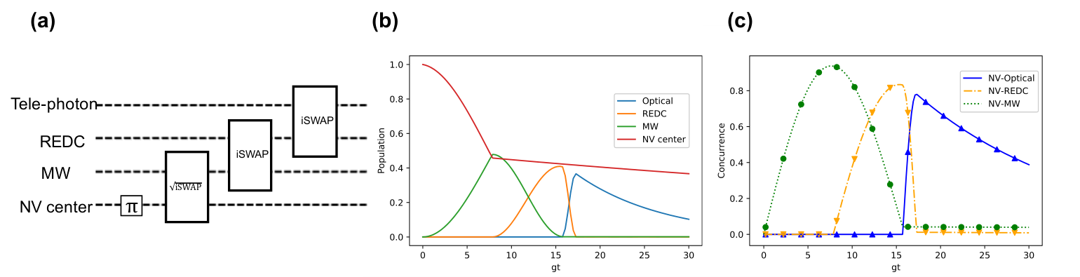
To entangle distant NV centers for applications such as quantum communication or remote sensing, generating entanglement of telecom photons and NV centers will be required. Here, we show that this could be realized in our proposed hybrid system with simple sequential gates.
Consider the Hamiltonian in the one-excitation subspace of the four modes. The evolution of two neighboring modes and (with coupling strength ) for a time will be given by the following matrix:
| (14) |
Interaction for a duration will correspond to the iSWAP gate used in the protocol of Sec. (III.1), while will yield the gate between subsystem and .
To create a maximally entangled Bell state one can initially prepare the NV ensemble in one excitation state while the other systems are in their ground state, and the following protocol can be implemented (Fig. 4 (a)): first a gate is applied while switching off by detuning the microwave resonator or changing the applied magnetic field, and this would generate entanglement between NV ensemble and microwave resonator; then two consecutive iSWAP gate can transfer the state from the microwave resonator to the REDC ensemble and then to telecom optical photon. A step-by-step analysis of the protocol is in Appendix C. Note this protocol could be implemented in reverse, with the excitation initially stored in the optical photon, but this will demand a long photon storage time, and the large decay in optical cavity will significantly worse the final entanglement generation (Appendix C).
In Fig. 4 we simulate this procedure with the same coupling and decay parameters as in the SWAP state transfer protocol discussed above. Entanglement between NV centers and telecom photons has a concurrence around 0.8. This could be further improved in practice since the parameters here are quite conservative. One can create an arbitrary entangled state (up to a relative phase factor) by changing the NV-MW interaction time from to a satisfying .
In this protocol the NV-photon entanglement generation rate is on the order of 1 MHz. In principle one could further extend the scheme to create remote NV-NV entanglement by sending the photons to a common station where they are measurement after passing through a balanced beam splitter Duan et al. 2001. When is small, the detection of one photon heralds the creation of the maximally-entangled state of two NV ensembles. For a typical photon detection efficiency et.al 2018, the corresponding generation rate can reach sub-kHZ. As the decoherence rate of entangled NV pairs can be greatly suppressed by control techniques including dynamical decoupling and double quantum driving Bauch et al. 2018, deterministic generation of entanglement might be feasible with our proposed interface et.al 2018.
IV Discussions
The two most important figures of merit of telecom photon-to-matter interface are the rate of entanglement generation (or state transfer) and the fidelity, or signal-to-noise ratio (SNR). In the spontaneous parametric down-conversion (SPDC) approach, applied to NV centers, the expected entanglement rate can be estimated from the probability of detecting a ZPL photon per resonant optical excitation and the conversion efficiency. Recent experiments Dréau et al. 2018 have achieved counts per excitation photon, with a total conversion efficiency of . Due to the broad phonon sideband in the NV emission spectrum, the ratio of ZPL photons sets an upper bound to the achievable rates.
Our protocol, instead, exploiting the microwave interface of NV centers, is not limited by the ZPL emission rate and does not need resonant optical driving for NV centers. The input microwave power and optical pump power could be increased to improve the microwave-optical signal conversion efficiency without the worry of the inverse conversion in the SPDC method. Still, as the coupling strengths between subsystems considered here are usually on the order of MHz, the rate of our protocol is limited by the gate time, which is considerably longer than the optical circle time. In principle, this could be improved in the future by implementing the scheme in ultra-strong coupling regime.
Another important metric is the final fidelity of the transferred state or the entanglement fidelity, which can be suppressed by system decoherence and noise. In the SPDC method, the SNR is limited by both detector dark counts and noise induced by pump laser field. As discussed above, our protocol can efficiently perform the tasks under realistic parameters and its conversion efficiency could reach near unit at low temperature (mK) Williamson et al. 2014; Fernandez-Gonzalvo et al. 2017. We point out that the protocol fidelities might be reduced by inhomogeneities in the coupling strengths and energy-level detuning, but these infidelities could be compensated by increasing the Q factors of the cavity and resonator, as discussed in Williamson et al. 2014. The induced noise would also include detector dark counts and scattering from the classical driving field. We note that even if our proposal involves more subsystems and thus seems to demand a more complex experiment, it does not require spectral filtering to reduce the pump noise as needed in SPDC, while at the same time it could enable more complex gates and operations, besides entanglement generation. Moreover, even if the microwave resonator should be at low temperature, in principle the NV centers could be at room temperature, since we don’t need resonant driving of optical transitions.
Photon indistinguishability is another important requirement for applications in quantum networks, such as entanglement swapping in quantum repeaters et.al 2018. The spectral diffusion of NV centers will result in a frequency difference in the optical transition, and charge fluctuations would further lead to long-term linewidth broadening Chu et al. 2014. In our approach, the output photon frequency difference would only depend on the optical cavity which could be improved by increasing the cavity fineness.
V Conclusion
We propose a hybrid system to interface an ensemble of NV centers to photons at telecom wavelength. The former can act as a quantum station while the latter can be used as flying qubits for applications in long distance quantum network in fibers without significant loss. We show that with REDC spin ensemble as a medium, we can effectively construct indirect coupling between NV centers and telecom photons. We proposed and numerically test applications to high fidelity quantum state transfer and efficient entanglement generation. The proposed schemes are within reach of current technologies. Such an interface would open new opportunities into future implementations of long-range quantum network with NV centers in diamond acting as quantum nodes.
Acknowledgements.
We would like to thank Akira Sone for helpful discussions. This work was in part supported by NSF grant EFRI ACQUIRE 1641064.Appendix A System dynamics in the bad cavity limit
By integrating the first two equations in Eq. (9) we get:
The task is to evaluate the integral . Note that the function:
will converge to the Dirac function in the limit of . With the product of a Dirac distribution and Heaviside function, we arrive at the relation:
Then the dynamics of operator and will have a simpler form:
Plugging these expressions into the the last two equations in Eq. (9), we reach Eq. (10) in the main text.
One can then simply get the dynamics of the two operators:
with . In the case of , the two spin ensemble modes will decay at the same rate.
Appendix B Spin ensemble interactions mediated by virtual photons
Assume the information is already stored in the REDC spin ensemble and here we consider its interaction with the NV spins, mediated by the microwave resonator that is far away detuned, with detuning . In the one-excitation basis of each mode, the effective Hamiltonian of the REDC-microwave-NV subsystem can be written as:
In the limit of , the microwave photons are virtually populated and we may take the coupling terms as perturbations, and reach the approximate Hamiltonian in the one-excitation basis of the two ensembles:
The corresponding eigenenergies and eigenstates are:
with . In the large detuning case, the coupling between two spin ensembles will be sufficiently lower compared to . Note that if one takes the photon excitation into consideration by solving the 3-by-3 matrix, the dark state actually corresponds to the case of zero microwave excitation, while the bright state has a term with one excitation, but it is suppressed by a factor .
Appendix C Entanglement generation
Here we show how entanglement could be generated between tele-photon and NV ensemble with sequential gates. Working in the one-excitation basis, at only the NV ensemble is in the one-excitation state and all other systems are in the vacuum state. Consider the system evolution for a time under the Hamiltonian stated in Eq. (6), while the REDC and microwave resonator are off-resonance. This corresponds to a gate, which will create entanglement between microwave photon with the NV center ensemble:
Then, by tuning and microwave resonator off resonance with the NV ensemble, the second iSWAP gate (corresponding to an interaction time ) would transfer the state of microwave resonator to REDC, while leaving the former in the ground state. In the subspace of these two subsystems, it can be shown:
Another iSWAP gate in succession will finally create entanglement between tele-photon and NV ensemble while leaving the REDC in its ground state:
This procedure could be reversed by starting with a number state in optical cavity. However, as shown in the figure below, the cavity decay would only yield a final NV-optical entanglement concurrence of 0.28, which means it is unlikely to success under the aforementioned decay parameters.
References
- Wehner et al. (2018) S. Wehner, D. Elkouss, and R. Hanson, Science 362 (2018), 10.1126/science.aam9288.
- Childress and Hanson (2013) L. Childress and R. Hanson, MRS Bulletin 38, 134–138 (2013).
- Degen et al. (2017) C. L. Degen, F. Reinhard, and P. Cappellaro, Rev. Mod. Phys. 89, 035002 (2017).
- et.al (2018) P. H. et.al, Nature 558, 268 (2018).
- De Greve et al. (2012) K. De Greve, L. Yu, P. L. McMahon, J. S. Pelc, C. M. Natarajan, N. Y. Kim, E. Abe, S. Maier, C. Schneider, M. Kamp, S. Höfling, R. H. Hadfield, A. Forchel, M. M. Fejer, and Y. Yamamoto, Nature 491, 421 EP (2012).
- Rakher et al. (2010) M. T. Rakher, L. Ma, O. Slattery, X. Tang, and K. Srinivasan, Nature Photonics 4, 786 EP (2010).
- Weber et al. (2019) J. H. Weber, B. Kambs, J. Kettler, S. Kern, J. Maisch, H. Vural, M. Jetter, S. L. Portalupi, C. Becher, and P. Michler, Nature Nanotechnology 14, 23 (2019).
- Bock et al. (2018) M. Bock, P. Eich, S. Kucera, M. Kreis, A. Lenhard, C. Becher, and J. Eschner, Nature Communications 9, 1998 (2018).
- Walker et al. (2018) T. Walker, K. Miyanishi, R. Ikuta, H. Takahashi, S. Vartabi Kashanian, Y. Tsujimoto, K. Hayasaka, T. Yamamoto, N. Imoto, and M. Keller, Phys. Rev. Lett. 120, 203601 (2018).
- Krutyanskiy et al. (2019) V. Krutyanskiy, M. Meraner, J. Schupp, V. Krcmarsky, H. Hainzer, and B. P. Lanyon, “Light-matter entanglement over 50 km of optical fibre,” (2019), arXiv:1901.06317 .
- Radnaev et al. (2010) A. G. Radnaev, Y. O. Dudin, R. Zhao, H. H. Jen, S. D. Jenkins, A. Kuzmich, and T. A. B. Kennedy, Nature Physics 6, 894 EP (2010).
- Maring et al. (2017) N. Maring, P. Farrera, K. Kutluer, M. Mazzera, G. Heinze, and H. de Riedmatten, Nature 551, 485 EP (2017).
- Yu et al. (2019) Y. Yu, F. Ma, X.-Y. Luo, B. Jing, P.-F. Sun, R.-Z. Fang, C.-W. Yang, H. Liu, M.-Y. Zheng, X.-P. Xie, W.-J. Zhang, L.-X. You, Z. Wang, T.-Y. Chen, Q. Zhang, X.-H. Bao, and J.-W. Pan, “Entanglement of two quantum memories via metropolitan-scale fibers,” (2019), arXiv:1903.11284 .
- Bogdanović et al. (2017) S. Bogdanović, S. B. van Dam, C. Bonato, L. C. Coenen, A.-M. J. Zwerver, B. Hensen, M. S. Z. Liddy, T. Fink, A. Reiserer, M. Lončar, and R. Hanson, Applied Physics Letters 110, 171103 (2017), https://doi.org/10.1063/1.4982168 .
- Dréau et al. (2018) A. Dréau, A. Tchebotareva, A. E. Mahdaoui, C. Bonato, and R. Hanson, Phys. Rev. Applied 9, 064031 (2018).
- Ikuta et al. (2014) R. Ikuta, T. Kobayashi, S. Yasui, S. Miki, T. Yamashita, H. Terai, M. Fujiwara, T. Yamamoto, M. Koashi, M. Sasaki, Z. Wang, and N. Imoto, Opt. Express 22, 11205 (2014).
- Maring et al. (2018) N. Maring, D. Lago-Rivera, A. Lenhard, G. Heinze, and H. de Riedmatten, “Quantum frequency conversion of memory-compatible single photons from 606 nm to the telecom c-band,” (2018), arXiv:1801.03727 .
- Barzanjeh et al. (2012) S. Barzanjeh, M. Abdi, G. J. Milburn, P. Tombesi, and D. Vitali, Phys. Rev. Lett. 109, 130503 (2012).
- Andrews et al. (2014) R. W. Andrews, R. W. Peterson, T. P. Purdy, K. Cicak, R. W. Simmonds, C. A. Regal, and K. W. Lehnert, Nature Physics 10, 321 EP (2014).
- Zhang et al. (2015) K. Zhang, F. Bariani, Y. Dong, W. Zhang, and P. Meystre, Phys. Rev. Lett. 114, 113601 (2015).
- Zhong et al. (2019) C. Zhong, Z. Wang, C. Zou, M. Zhang, X. Han, W. Fu, M. Xu, S. Shankar, M. H. Devoret, H. X. Tang, and L. Jiang, “Heralded generation and detection of entangled microwave–optical photon pairs,” (2019), arXiv:1901.08228 .
- Tsang (2010) M. Tsang, Phys. Rev. A 81, 063837 (2010).
- Li and Li (2018) C.-H. Li and P.-B. Li, Phys. Rev. A 97, 052319 (2018).
- Fan et al. (2018) L. Fan, C.-L. Zou, R. Cheng, X. Guo, X. Han, Z. Gong, S. Wang, and H. X. Tang, “Superconducting cavity electro-optics: a platform for coherent photon conversion between superconducting and photonic circuits,” (2018), arXiv:1805.04509 .
- Zhong et al. (2016) T. Zhong, J. Rochman, J. M. Kindem, E. Miyazono, and A. Faraon, Opt. Express 24, 536 (2016).
- Zhong et al. (2017) T. Zhong, J. M. Kindem, J. Rochman, and A. Faraon, Nature Communications 8, 14107 EP (2017).
- Probst et al. (2013) S. Probst, H. Rotzinger, S. Wünsch, P. Jung, M. Jerger, M. Siegel, A. V. Ustinov, and P. A. Bushev, Phys. Rev. Lett. 110, 157001 (2013).
- Williamson et al. (2014) L. A. Williamson, Y.-H. Chen, and J. J. Longdell, Phys. Rev. Lett. 113, 203601 (2014).
- O’Brien et al. (2014) C. O’Brien, N. Lauk, S. Blum, G. Morigi, and M. Fleischhauer, Phys. Rev. Lett. 113, 063603 (2014).
- Everts et al. (2018) J. R. Everts, M. C. Berrington, R. L. Ahlefeldt, and J. J. Longdell, “Microwave to optical photon conversion via fully concentrated rare-earth ion crystals,” (2018), arXiv:1812.03246 .
- Fernandez-Gonzalvo et al. (2015) X. Fernandez-Gonzalvo, Y.-H. Chen, C. Yin, S. Rogge, and J. J. Longdell, Phys. Rev. A 92, 062313 (2015).
- Fernandez-Gonzalvo et al. (2017) X. Fernandez-Gonzalvo, S. P. Horvath, Y.-H. Chen, and J. J. Longdell, “Cavity enhanced raman heterodyne spectroscopy in er:yso for microwave to optical signal conversion,” (2017), arXiv:1712.07735 .
- Blum et al. (2015) S. Blum, C. O’Brien, N. Lauk, P. Bushev, M. Fleischhauer, and G. Morigi, Phys. Rev. A 91, 033834 (2015).
- Thiel et al. (2011) C. Thiel, T. Böttger, and R. Cone, Journal of Luminescence 131, 353 (2011), selected papers from DPC’10.
- Holstein and Primakoff (1940) T. Holstein and H. Primakoff, Phys. Rev. 58, 1098 (1940).
- Kubo et al. (2010) Y. Kubo, F. R. Ong, P. Bertet, D. Vion, V. Jacques, D. Zheng, A. Dréau, J.-F. Roch, A. Auffeves, F. Jelezko, J. Wrachtrup, M. F. Barthe, P. Bergonzo, and D. Esteve, Phys. Rev. Lett. 105, 140502 (2010).
- Sandner et al. (2012) K. Sandner, H. Ritsch, R. Amsüss, C. Koller, T. Nöbauer, S. Putz, J. Schmiedmayer, and J. Majer, Phys. Rev. A 85, 053806 (2012).
- et.al (2014) S. P. et.al, Nature Physics 10, 720EP (2014).
- Cirac (1992) J. I. Cirac, Phys. Rev. A 46, 4354 (1992).
- van Woerkom et al. (2018) D. J. van Woerkom, P. Scarlino, J. H. Ungerer, C. Müller, J. V. Koski, A. J. Landig, C. Reichl, W. Wegscheider, T. Ihn, K. Ensslin, and A. Wallraff, Phys. Rev. X 8, 041018 (2018).
- Sandberg et al. (2008) M. Sandberg, C. M. Wilson, F. Persson, T. Bauch, G. Johansson, V. Shumeiko, T. Duty, and P. Delsing, Applied Physics Letters 92, 203501 (2008), https://doi.org/10.1063/1.2929367 .
- Jakobi et al. (2016) I. Jakobi, P. Neumann, Y. Wang, D. B. R. Dasari, F. El Hallak, M. A. Bashir, M. Markham, A. Edmonds, D. Twitchen, and J. Wrachtrup, Nature Nanotechnology 12, 67 EP (2016).
- Wang and Clerk (2012) Y.-D. Wang and A. A. Clerk, Phys. Rev. Lett. 108, 153603 (2012).
- Li et al. (2017) B. Li, P.-B. Li, Y. Zhou, S.-L. Ma, and F.-L. Li, Phys. Rev. A 96, 032342 (2017).
- Berry (2009) M. V. Berry, Journal of Physics A: Mathematical and Theoretical 42, 365303 (2009).
- Baksic et al. (2016) A. Baksic, H. Ribeiro, and A. A. Clerk, Phys. Rev. Lett. 116, 230503 (2016).
- Zhang et al. (2018) H. Zhang, X.-K. Song, Q. Ai, H. Wang, G.-J. Yang, and F.-G. Deng, “Fast and robust quantum control for multimode interactions by using shortcuts to adiabaticity,” (2018), arXiv:1809.00102 .
- Duan et al. (2001) L. M. Duan, M. D. Lukin, J. I. Cirac, and P. Zoller, Nature 414, 413 EP (2001).
- Bauch et al. (2018) E. Bauch, C. A. Hart, J. M. Schloss, M. J. Turner, J. F. Barry, P. Kehayias, S. Singh, and R. L. Walsworth, Phys. Rev. X 8, 031025 (2018).
- Chu et al. (2014) Y. Chu, N. de Leon, B. Shields, B. Hausmann, R. Evans, E. Togan, M. J. Burek, M. Markham, A. Stacey, A. Zibrov, A. Yacoby, D. Twitchen, M. Loncar, H. Park, P. Maletinsky, and M. Lukin, Nano Letters 14, 1982 (2014), pMID: 24588353, https://doi.org/10.1021/nl404836p .
*