On the Stability of Periodic Traveling Waves for the Modified Kawahara Equation

See Proposition 4.12 in [7]. ∎

Given $v\in\left\{\phi^{\prime}\right\}^{\perp}$, let us define $z=v-\zeta w,$ where $w=\frac{Q^{\prime}(\phi)}{||Q^{\prime}(\phi)||_{L^{2}_{per}}}$ and $\zeta=\langle v,w\rangle$. Since $\langle Q^{\prime}(\phi),\phi^{\prime}\rangle=0$, it is easy to see that $z\in\Upsilon_{0}\cap\left\{\phi^{\prime}\right\}^{\perp}$. Thus, Lemma 2.3 implies

Choosing $N>0$ depending only on $\phi$ such that

we obtain, using (2.2)-(2.4) the following inequality

where $\tau>0$ is a constant that does not depend on $v$. The proof is thus completed. ∎

First, note that from the definition of $V$ it follows that

for all $u,v\in X$. In particular, $\langle V^{\prime\prime}(\phi)v,v\rangle=\langle\mathcal{L}v,v\rangle+2N\langle Q^{\prime}(\phi),v\rangle^{2}.$ Consequently, from Lemma 2.4 we get

for all $v\in\left\{\phi^{\prime}\right\}^{\perp}$.

On the other hand, a Taylor expansion of $V$ around $\phi$ reveals that

where $\lim\limits_{u\to\phi}\frac{h(u)}{||u-\phi||_{X}^{2}}=0$. Thus, we can choose $\alpha_{1}>0$ such that

where $B_{\alpha_{1}}(\phi)=\left\{u\in X;||u-\phi||_{X}<\alpha_{1}\right\}$.

Since $V(\phi)=0$ and $V^{\prime}(\phi)=0$, we have from $(\ref{eq001})-(\ref{limit1})$ that $V(u)\geq\frac{\tau}{4}\rho(u,\phi)^{2},$ for all $u\in B_{\alpha_{1}}(\phi)$ such that $(u-\phi)\in\left\{\phi^{\prime}\right\}^{\perp}.$

Now, let us define the smooth map $S:X\times\mathbb{R}\rightarrow\mathbb{R}$ given by $S(u,r)=\langle u(\cdot-r),\phi^{\prime}\rangle$. Since $S(\phi,0)=0$ and $\frac{\partial S}{\partial r}(\phi,0)=-\langle\phi^{\prime},\phi^{\prime}\rangle\neq 0$, we guarantee, from the implicit function theorem, the existence of $\alpha_{2}>0$, $\delta_{0}>0$ and a unique $C^{1}-$map $r:B_{\alpha_{2}}(\phi)\rightarrow(-\delta_{0},\delta_{0})$ such that $r(\phi)=0$ and $S(u,r(u))=0$, for all $u\in B_{\alpha_{2}}(\phi)$. Consequently, $(u(\cdot-r(u))-\phi)\in\left\{\phi^{\prime}\right\}^{\perp}$, for all $u\in B_{\alpha_{2}}(\phi)$. The remainder of the proof follows from similar arguments as in [2] (see also [7]).

∎

Let $\alpha>0$ be the constant such that Lemma 2.5 holds. Since $V$ is continuous at $\phi$, for a given $\varepsilon>0$, there exists $\delta\in(0,\alpha)$ such that if $||u_{0}-\phi||_{X}<\delta$ one has $V(u_{0})=V(u_{0})-V(\phi)<D\varepsilon^{2},$ where $D>0$ is the constant in Lemma 2.5.

The continuity in time of the function $\rho(u(t),\phi)$ allows to choose $T>0$ such that

Thus, one obtains $u(t)\in U_{\alpha}$, for all $t\in[0,T)$. Combining Lemma 2.5 and the fact that $V(u(t))=V(u_{0})$ for all $t\geq 0$, we have

Next, we prove that $\rho(u(t),\phi)<\alpha$, for all $t\in[0,+\infty)$, from which one concludes the orbital stability. Indeed, let $T_{1}>0$ be the supremum of the values of $T>0$ for which $(\ref{subalpha})$ holds. To obtain a contradiction, suppose that $T_{1}<+\infty$. By choosing $\varepsilon<\frac{\alpha}{2}$ we obtain, from $(\ref{estepsilon1})$ that $\rho(u(t),\phi)<\frac{\alpha}{2},$ for all $t\in[0,T_{1})$. Since $t\in(0,+\infty)\mapsto\rho(u(t),\phi)$ is continuous, there is $T_{0}>0$ such that $\rho(u(t),\phi)<\frac{3}{4}\alpha<\alpha$, for $t\in[0,T_{1}+T_{0})$, contradicting the maximality of $T_{1}$. Therefore, $T_{1}=+\infty$ and the theorem is established. ∎

The proof of this result can be found in [5, Theorem 4.1]. See also [1] for the continuous case. ∎

In fact, according with [11], solution $\phi$ in (3.3) has the Fourier expansion $\phi(x)=a+\sum_{n=1}^{\infty}n\Gamma\mbox{csch}\left(\frac{n\pi K(k^{\prime})}{K(k)}\right)\cos\left(\frac{2\pi n}{L}x\right),$ where $\Gamma=\frac{b\pi^{2}}{K(k)^{2}}$ and $k^{\prime}=\sqrt{1-k^{2}}$. Therefore, the Fourier coefficients of $\phi$ are given by

By considering $g_{k}(x):=\frac{\Gamma}{2}x\mbox{csch}\left(\frac{x\pi K(k^{\prime})}{K(k)}\right)=\frac{12\sqrt{10}\pi^{2}}{L^{2}}x\mbox{csch}\left(\frac{x\pi K(k^{\prime})}{K(k)}\right)$, $x\in\mathbb{R}$, it is possible to see that $\frac{\partial^{2}}{{\partial x}^{2}}(\log{g_{k}(x)})<0$, for all $x\in{\mathbb{R}}$ and $k\in(0,1)$ (see Figure 3.1).

So, using Proposition 3.2, we obtain that $\mathcal{L}$ has only one negative eigenvalue which is simple and zero is a simple eigenvalue whose eigenfunction is $\phi^{\prime}$. Therefore, we have that $(H)$ holds.

The next step is to find $\Phi$ as in Lemma 2.3. In fact, we consider $\Phi=\frac{\partial}{\partial k}\phi$. Note that, using (3.2), we have

Equality $(\ref{I1})$ inspires us from $(\ref{functQ})$ in choosing $\nu=\frac{\partial\omega}{\partial k}$ and $\mu=\frac{\partial A}{\partial k}$ to get $Q(u)=\frac{\partial\omega}{\partial k}F(u)+\frac{\partial A}{\partial k}M(u)$ and $\mathcal{L}\Phi=-Q^{\prime}(\phi)$. Thus, we have $\langle\mathcal{L}\Phi,\varphi\rangle=-\langle Q^{\prime}(\phi),\varphi\rangle=0$, for all $\varphi\in\Upsilon_{0}$ and

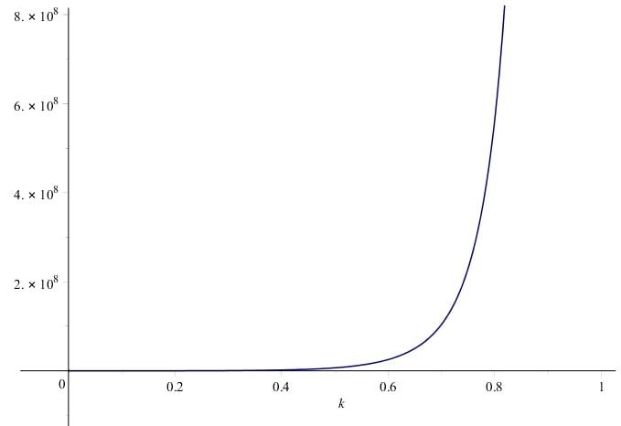
Using the explicit form (3.3), it is possible to deduce that $M(\phi)=aL$ and $F(\phi)=\frac{480K(k)^{3}}{L^{4}}\left[k^{2}L+\frac{2L(k^{4}-k^{2}+1)}{3}K(k)\right].$ Therefore, we are able to obtain

where $f$ is a complicated positive function depending smoothly on $k\in(0,1)$ (see Figure 3.2). This proves the required in Lemma 2.3. From Theorem 2.6, we conclude that $\phi$ is orbitally stable in $H_{per}^{2}([0,L])$ by the periodic flow of (3.1).

∎

References

- [1] J.P. Albert, Positivity properties and stability of solitary-wave solutions of model eqautions for long waves, Comm. Part. Diff. Equat., 17 (1992), pp. 1-22.
- [2] G. Alves, F. Natali and A. Pastor, Sufficient conditions for orbital stability of periodic traveling waves, J. Diff. Equat., 267 (2019), pp. 879-901.
- [3] T.P. Andrade, F. Crisófani and F. Natali, Orbital Stability of Periodic Traveling Wave Solutions for the Kawahara Equation, J. Math. Phys., 58 (2017), pp. 051504.
- [4] T.P. Andrade and A. Pastor, Orbital stability of periodic traveling-wave solutions for the BBM equation with fractional nonlinear term, Phys. D, 317 (2016), pp. 43-58.
- [5] J. Angulo and F. Natali, Positivity properties of the Fourier transform and the stability of periodic travelling-wave solutions, SIAM J. Math. Anal., 40 (2008), pp. 1123-1151.
- [6] P.F. Byrd and M.D. Friedman. Handbook of elliptic integrals for engineers and scientists, 2nd ed., Springer, New York, (1971).
- [7] F. Cristófani, F. Natali and A. Pastor, Orbital stability of periodic traveling-wave solutions for the Log-KdV equation, J. Differential Equations, 263 (2017), pp. 2630–2660.
- [8] M. Grillakis, J. Shatah and W. Strauss, Stability theory of solitary waves in the presence of symmetry I. J. Funct. Anal. 74 (1987), pp. 160-197.
- [9] K. Kano and T. Nakayama, An exact solution of the wave equation , J. Phys. Soc. Jpn., 50 (1981), pp. 361-362.
- [10] C. Kwak, Well-posedness issues on the periodic modified Kawahara equation, preprint (2019), https://arxiv.org/abs/1902.08946.
- [11] A. Kiper, Fourier series coefficients for powers of the Jacobian elliptic functions, Math. Comput., 43 (1984), pp. 247-259.
- [12] F. Natali and A. Pastor, The fourth-order dispersive nonlinear Schrödinger equation: orbital stability of a standing wave, SIAM J. Appl. Dyn. Systems, 14 (2015), pp. 1326–1347.
- [13] E.J. Parkes, B.R. Duffy and P.C. Abbot, The Jacobi elliptic-function method for finding periodic-wave solutions to nonlinear evolution equations. Phys. Lett. A, 295 (2002), pp. 280-286.
- [14] C.A. Stuart, Lectures on the orbital stability of standing waves and applications to the nonlinear Schrödinger equation, Milan J. Math. 76 (2008), pp. 329–-399.
- [15] A. Zygmund, Trigonometrical series, Warszawa-Lwów, Instytut Matematyczny Polskiej Akademi Nauk, (1935).