Phase structure of three flavor QCD in external magnetic fields using HISQ fermions

Mapping out QCD phase diagram is one of the most important goals in high energy nuclear physics. QCD thermodaynamics has several controllable parameters, temperature $T$, baryon chemical potential and in addition quark masses $m_{\text{ud}},\;m_{\text{s}}$ for theoretical studies. Quark mass is a relevant parameter and it affects the order of QCD phase transition because chiral symmetry is controlled by the mass, which is summarized in the Columbia plot [1, 2]. One can introduce an extra parameter, e.g. the background magnetic field $eB$ [3], which can be generated in the early stage of relativistic heavy ion collision experiments. The presence of the magnetic field breaks flavor symmetry and rotational symmetry, and the magnitude of the magnetic field is expected to reach to QCD scale so the chiral phase transition would be affected.

From lattice QCD simulations with external magnetic field at the physical pion mass, especially using stout smeared staggered actions, the inverse magnetic catalysis has been found around the pseudo critical temperature [4]. Recently, the origin of the inverse magnetic catalysis, in particular the relation between the decreasing of pseudo critical temperature and the non-monotonic behavior of chiral condensate around the pseudo critical temperature has been studied in details in $N_{f}$=2+1 QCD with a few values of heavy pions using stout staggered fermions [5]. A previous lattice study with an effective model suggested a new critical end point along with the magnetic field. They employed stout smeared staggered quarks with physical pion mass for their lattice calculation and gluonic effective model for predictions [6]. The new critical point is predicted to appear $eB\sim 10\;\text{GeV}^{2}$ so it is practically difficult to reach such a strong magnetic field using lattice calculations since the maximum of the magnetic field is bounded by the cutoff $a^{-1}$. The cutoff at the critical point is $a^{-1}\sim 2.4$ GeV. However, there is a chance to observe the first oder phase transition if a system is in proximity to a critical point. This is because, according to our previous work using the standard staggered fermions, the magnetic field tends to make the phase transition stronger [7].

In this work, we investigate mass degenerate three flavor QCD, namely, $m=m_{\text{ud}}=m_{\text{s}}$ and around $SU(3)$ chiral limit. We performed simulations with quark masses corresponding to pion masses of $320$ MeV and $80$ MeV in the continuum limit. The results with the heavier quark is used to check the cutoff effects because that mass corresponds to similar mass regime to the our previous work with the standard staggered fermion, while those with the lighter quark are used to explore criticality as it is much closer to the first order regime compared to the physical pion mass regime.

This proceedings is organized as follows. In next section, we introduce our numerical setup, which includes the implementation of the external field on the lattice with smeared links. In section 3, we review a stochastic estimator to calculate the Dirac spectrum with the external field. In section 4, we show our results. In section 5, we summarize our observations.

Here we review the stochastic spectrum estimator [12, 13, 14, 15]. Let us denote $n[s,t]$ as the number of eigenvalues of a Hermitian operator $\tilde{D}=\tilde{D}(A)$ having eigenvalues in $[-1,1]$ in a range $[s,t]$. We use a ramp function $h_{[s,t]}(x)$ with a support $[s,t]$, i.e.

By definition, the number is $n[s,t]=\sum_{j}\langle h_{[s,t]}(\lambda_{j}^{\tilde{D}(A)})\rangle_{A}$, where $\left\langle\cdots\right\rangle_{A}$ is an ensemble average and $\lambda_{j}^{\tilde{D}(A)}$ is $j$–th eigenvalue of $\tilde{D}$ on a gauge configuration $A$. Summation over all of eigenvalues can be represented by trace operation and,

where $h_{[s,t]}(x)\approx\sum_{n}^{p}\gamma^{(n)}_{[s,t]}T_{n}(x)$ and $T_{n}(x)$ is the Chebyshev polynomial. $\xi_{k}$ is $k$–th random vector and $N_{r}$ is the number of random vectors. During the derivation, we have approximated trace operation as a Monte-Carlo average of random vectors. In actual calculation we introduce the Jackson dumping factor to suppress the Gibbs phenomena in the most right hand side in (10) as in Ref.[14].

In order to apply the Chebyshev expansion to calculate the Dirac spectrum, we take

where $\lambda^{D^{\dagger}D}_{\text{max}}$ and $\lambda^{D^{\dagger}D}_{\text{min}}$ are the maximum and minimum eigenvalues of a positive Hermitian operator $D^{\dagger}D$, respectively. Thus the range of eigenvalue of $\tilde{D}$ is restricted in $[-1,1]$. By taking the square root of ${\lambda^{D^{\dagger}D}}$, we reconstruct the Dirac spectrum through the following equation,

where $\sqrt{\lambda^{D^{\dagger}D}}=\sqrt{(\frac{\lambda^{D^{\dagger}D}_{max}-\lambda^{D^{\dagger}D}_{min}}{2})s+\frac{\lambda^{D^{\dagger}D}_{max}+\lambda^{D^{\dagger}D}_{min}}{2}}$ and $\sqrt{\lambda^{D^{\dagger}D}}+\delta=\sqrt{(\frac{\lambda^{D^{\dagger}D}_{max}-\lambda^{D^{\dagger}D}_{min}}{2})t+\frac{\lambda^{D^{\dagger}D}_{max}+\lambda^{D^{\dagger}D}_{min}}{2}}$. Here $V$ is the volume of the system and for the step size $\delta$ we have $\delta=0.0005$. The eigenvalues are $D\psi_{j}=i\lambda_{j}\psi_{j}$ and

where $\psi_{j}$ is an eigenvector. Using the Dirac spectrum, one can reconstruct the chiral condensate,

except for finite volume corrections. This $\left\langle\overline{\psi}\psi\right\rangle_{\text{spec}}$ is used in the calculation of the relative increase of chiral condensate $r$.

Here we show our results for $m_{\pi}=320$ MeV. In general $m_{\pi}=80$ MeV system shows qualitatively similar results with $m_{\pi}=320$ MeV system except for behavior of the pseudo critical temperature in external magnetic fields so we just address some results on $m_{\pi}=80$ MeV system later.

Our results for the chiral condensate susceptibility (left panel) and corresponding Binder cumulant (right panel) for $m_{\pi}=320$ MeV are shown in Fig. 1. It can be clearly seen that the peak location of the chiral susceptibility moves to lower temperature in stronger magnetic field and the peak heights increases with the magnetic field. The Binder cumulant shows that the system lies in the crossover regime.

In Fig. 2 we show the Dirac spectra with $m_{\pi}=320$ MeV at just above the critical temperature. Dirac spectra with the magnetic field in both sea and dynamical quarks, sea quark only and valence quark only, obtained using (4), (5) and (6), are shown from left to right panel in Fig. 2. For $N_{b}>0$, left four panels are consistent with inverse magnetic catalysis while valence ones only show normal magnetic catalysis behavior.

The relative increase of chiral condensate $r$ with $m_{\pi}=320$ MeV in two different phases is shown in Fig. 3. The left panel is for the low temperature phase. All of them monotonically increases as a function of $N_{b}$, namely they show normal magnetic catalysis. Right panel shows the $r$ dependence on $N_{b}$ in the high temperature phase. We can see that contributions from the dynamic sea quarks show non-montonical behavior. This indicates that the inverse magnetic catalysis seems to originate from contribution from dynamic sea quarks. This is consistent with the results from Ref. [4].

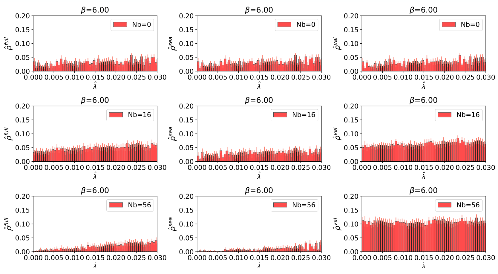
We also measure the chiral condensate and its susceptibility for $m_{\pi}=80$ MeV system. The susceptibility shows nontrivial dependence of peak location on $N_{b}$, namely, first the critical temperature increases and decreases. Except for nontrivial dependence of the susceptibility for the magnetic field, results shows qualitatively similar behavior. It might be physical phenomena around chiral limit but $m_{\pi}L\sim 1.7<4$, so it could be finite volume effects and further investigations are needed. We observe that the Dirac spectrum is qualitatively similar to the heavier case.

We have performed simulations of $N_{f}=3$ QCD in external magnetic fields using the HISQ action on $16^{3}\times 6$ lattices. Two different values of quark masses are chosen corresponding to $m_{\pi}$=320 MeV and 80 MeV. We have observed inverse magnetic catalyses in both cases of $m_{\pi}=320$ MeV and $80$ MeV. Except for the dependence of the pseudo critical temperature on the background magnetic field, two systems show qualitatively similar behavior. On the other hand, $m_{\pi}=80$ MeV data shows non monotonic dependence on the external field. However, this result is suspected coming from finite volume effects and further investigation is needed.

We would like to thank a lattice group in Eötvös university for fruitful discussions. The work of AT was supported in part by NSFC under grant no. 11535012 and the RIKEN Special Postdoctoral Researcher program. The numerical simulations have been performed on the GPU cluster in the Nuclear Science Computing Center at CCNU, and Tianhe II supercomputing center in Guangzhou. This work was supported through Contract No. de-sc0012704 with the U.S. Department of Energy, and through the Scientific Discovery through Advanced Computing (SciDAC) program funded by the U.S. Department of Energy, Office of Science, Office of Nuclear Physics. CS acknowledge support by the Deutsche Forschungsgemeinschaft (DFG, German Research Foundation) – project number 315477589 – TRR 211.

References

- [1] Robert D. Pisarski and Frank Wilczek. Remarks on the Chiral Phase Transition in Chromodynamics. Phys. Rev., D29:338–341, 1984.
- [2] Frank R. Brown, Frank P. Butler, Hong Chen, Norman H. Christ, Zhi-hua Dong, Wendy Schaffer, Leo I. Unger, and Alessandro Vaccarino. On the existence of a phase transition for QCD with three light quarks. Phys. Rev. Lett., 65:2491–2494, 1990.
- [3] Pedro Costa, Marcio Ferreira, and Constanca Providencia. Magnetized QCD phase diagram: critical end points for the strange quark phase transition driven by external magnetic fields. PoS, Hadron2017:161, 2018.
- [4] Falk Bruckmann, Gergely Endrodi, and Tamas G. Kovacs. Inverse magnetic catalysis and the Polyakov loop. JHEP, 04:112, 2013.
- [5] Massimo D’Elia, Floriano Manigrasso, Francesco Negro, and Francesco Sanfilippo. QCD phase diagram in a magnetic background for different values of the pion mass. Phys. Rev., D98(5):054509, 2018.
- [6] Gergely Endrodi. Critical point in the QCD phase diagram for extremely strong background magnetic fields. JHEP, 07:173, 2015.
- [7] Akio Tomiya, Heng-Tong Ding, Swagato Mukherjee, Christian Schmidt, and Xiao-Dan Wang. Chiral phase transition of three flavor QCD with nonzero magnetic field using standard staggered fermions. EPJ Web Conf., 175:07041, 2018.
- [8] MH Al-Hashimi and U-J Wiese. Discrete accidental symmetry for a particle in a constant magnetic field on a torus. Annals of physics, 324(2):343–360, 2009.
- [9] Kurt Binder. Critical properties from monte carlo coarse graining and renormalization. Physical Review Letters, 47(9):693, 1981.
- [10] A. Bazavov, H. T. Ding, P. Hegde, F. Karsch, E. Laermann, Swagato Mukherjee, P. Petreczky, and C. Schmidt. Chiral phase structure of three flavor QCD at vanishing baryon number density. Phys. Rev., D95(7):074505, 2017.
- [11] Massimo D’Elia and Francesco Negro. Chiral Properties of Strong Interactions in a Magnetic Background. Phys. Rev., D83:114028, 2011.
- [12] Leonardo Giusti and Martin Luscher. Chiral symmetry breaking and the Banks-Casher relation in lattice QCD with Wilson quarks. JHEP, 03:013, 2009.
- [13] Zoltan Fodor, Kieran Holland, Julius Kuti, Santanu Mondal, Daniel Nogradi, and Chik Him Wong. New approach to the Dirac spectral density in lattice gauge theory applications. PoS, LATTICE2015:310, 2016.
- [14] Guido Cossu, Hidenori Fukaya, Shoji Hashimoto, Takashi Kaneko, and Jun-Ichi Noaki. Stochastic calculation of the Dirac spectrum on the lattice and a determination of chiral condensate in 2+1-flavor QCD. PTEP, 2016(9):093B06, 2016.
- [15] Philippe de Forcrand and Benjamin Jager. Alternatives to the stochastic “noise vector” approach. EPJ Web Conf., 175:14022, 2018.