DSAL-GAN: Denoising based Saliency Prediction with Generative Adversarial Networks

The problem of denoising can mathematically be formulated as $x=D.y$. The $x$ and $y$ denote the noisy and clean image (without noise perturbations) and $D$ represents the noise matrix which degrades the clean image. Clean image $y$ can be obtained by taking inverse of the noise matrix. The formulation to obtain denoised image $y$ is:

Where $f_{d}$ is denoising function. The saliency map can be obtained using the following equation:

Where $z$ is the saliency map of clean image $y$ obtained using denoising function on $x$. The $f_{SOD}$ function is responsible for localization of saliency map.

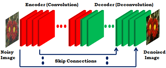
As shown in the Fig. 2, the denoising network maps the noisy image $x$ to a clean (denoised) image $y$. The generator $G1$ learns to generate image $y_{predicted}$ from input noisy image $x$, while the discriminator network $D1$ learns to differentiate between $y_{predicted}=y_{p}$ and $y$ (Ground Truth). Here, the generator architecture is similar as given in [6], and shown in Fig. 3. The content loss (L2 Loss) of the generator can be represented as,

The adversarial loss can be formulated as,

Total loss for the denoising network is calculated as,

The network for saliency detection shown in the Fig. 2 is the extended version of the SalGAN [5]. The network is optimized for three different losses naming, content loss i.e., binary cross entropy (BCE), adversarial loss and cyclic consistency loss. Cyclic consistency loss is introduced to limit the space of possible mapping function. The three losses can be formulated as,

The overall joint optimization objective of training the network can be formulated as,

The specification of discriminator [6] architecture used for denoising and salient object detection is given in Table. 1 respectively. The generator [6] architecture used for salient object detection is given in Table. 2. The architecture given in Fig. 3 is also used for generator3 (G3) to learn reverse mapping from saliency map to corresponding clean image.

We initialise end-to-end coupled network i.e., DSAL-GAN for joint optimization of denoising and saliency prediction by taking pre-trained weights of network1 and network2 as given in Fig. 2. We consider pre-trained weights as initial weights to finetune the combined network into an end-to-end manner.

We have trained our model on benchmark datasets such as SOD [7], MSRA 10k [8] and ECSSD [9]. We have created a synthetic dataset using the input images from these datasets and degraded them using Gaussian noise with variance ranging from [10, 30, 50, 80]. The experimental results are obtained on these synthesized datasets for various baseline saliency detection models.

The comparison of DSAL-GAN with other state-of-the-art saliency detection framework is shown in Fig. 4 (for illustration purposes we have shown results for $\sigma$=50 only). The performance of the proposed framework shows performance gain over the other state of the art saliency detection frameworks for noisy images. Table 3 represents the comparative analysis between these techniques over several performance evaluation metrics average F-measure (aveF), maximum F-measure (maxF), Area under the curve (AUC), Mean Average Error (MAE). The performance of the proposed framework shows far more effective detection of salient regions as compared to the state of the art saliency detection frameworks for noisy images. The proposed framework provides an improvement of $\sim 10\%$ and $16\%$ in aveF, $\sim 9.5\%$ and $16\%$ in maxF, and $\sim 9.6\%$ and $21\%$ in AUC and a drop of $\sim 38\%$ and $47\%$ in MAE with respect to Sal-GAN and Deep Saliency respectively for images having noise variance, $\sigma=50$. Performance gain in AUC represents the increase in the pixel classification accuracy. It can be evidently observed that the proposed framework outperforms various state of the art saliency detection frameworks on noise induced synthetic dataset. The experimental results validates that there is decrease in AUC with increase in noise as shown in Tab. 4.

Baseline: We have benchmarked the performance of DSAL-GAN against the state-of-the-art frameworks like Sal-GAN and Deep Saliency on our synthetic dataset. We observe a performance drop in F1-score, AUC, MAE metrics for Sal-GAN and Deep Saliency, when they are trained on our synthetic dataset.