Nested Dithered Quantization for Communication Reduction in Distributed Training

Throughout the paper, bold lowercase letters represent vectors and the $i$-th element of the vector $\bm{x}$ is denoted as $x_{i}$. Matrices are denoted by bold capital letters such as $\bm{X}$, with the $(i,j)$-th element represented by $X_{i,j}$ or $[\bm{X}]_{i,j}$. Given a real number $x\in\mathbb{R}$, $\left\lfloor x\right\rceil$ is the nearest integer to $x$. For a random variable $u$, $u\sim\mathcal{U}[a,b]$ if its probability distribution is uniform over interval $[a,b]$ and $u\sim\mathcal{N}(\mu,\sigma^{2})$ if it follows a Gaussian distribution with mean $\mu$ and variance $\sigma^{2}$.

It is well-known that the error in ordinary quantization especially when the number of quantization levels is low, depends on the input signal and is not necessarily uniformly distributed. In Dithered Quantization, a (pseudo-)random signal called dither is added to the input signal prior to quantization. Adding this controlled perturbation can cause the statistical behavior of the quantization error to be more desirable [11, 12, 13].

Let $Q(\cdot)$ be an M-level uniform quantizer with quantization step size of $\Delta$, i.e., $Q(v)=\Delta\left\lfloor v/\Delta\right\rceil$ where $\left\lfloor\alpha\right\rceil$ is the nearest integer to $\alpha$. The dithered quantizer is defined as follows;¹¹ 1 Throughout the paper, we assume that all quantizers are centered around $0$. This is the case also for ternary [6] and stochastic quantizations [5].

It is common to consider $\mathcal{U}[\Delta/2,\Delta/2]$ as the distribution of the random dither signal. It can be easily verified that this choice of the dither signal satisfies the conditions of Thm. 1, and it does not increase the bound of the quantization error, i.e, $|\tilde{x}-x|\leq\Delta/2$ which is the same as the traditional uniform quantization with the same step size.

In some cases, the receiver may not be able to reproduce the dither signal to subtract from $Q(x+u)$. Hence, quantization is simply defined as as $\tilde{x}_{h}=Q(x+u)$. We refer to this approach as the half-dithered quantization as the dither signal is applied only to the quantizer, not the reconstruction of $x$. In this case, the quantization error is not necessarily independent of the signal, however by an appropriate choice of the dither signal, the moments of the quantization error will be independent [12]. For example, if the dither signal $u$ is the sum of $k$ independent random variables, each having uniform distribution $\mathcal{U}[-\Delta/2,\Delta/2]$, then the $k$-th moment of the quantization error, $\epsilon=x-\tilde{x}_{h}$, would be independent of the signal, given by $\operatorname{\mathbb{E}}\left[\epsilon^{k}|x\right]=\operatorname{\mathbb{E}}\left[\epsilon^{k}\right]=(k+1)\frac{\Delta^{2}}{12}$.

Here, we briefly overview the definition and some properties of the nested quantization. Especially we focus on the one dimensional case as our algorithm is based on scalar quantization.

As a result, the centers of the quantization bins in the coarse quantizer is a subset of those of the fine quantizer. In the one dimensional case, if $Q_{1}$ and $Q_{2}$ have quantization step sizes equal to $\Delta_{1}$ and $\Delta_{2}$, respectively, it can be easily verified that they are nested if and only if there exists a constant integer $k>1$ such that $\Delta_{2}=k\Delta_{1}$. For the definition and properties of higher dimensional nested quantization using lattices please refer to [14, 15] and references therein.

We consider the dithered quantization of SG (DQSG) as follows: Let $Q(\cdot)$ be a uniform quantizer with quantization step size $\Delta$, and $\bm{u}\sim\mathcal{U}[-\Delta/2,\Delta/2]$ be the random dither signal. The dithered quantized SG is given by

where the scale factor $\kappa=\|\bm{g}\|_{\infty}=\max_{i}|g_{i}|$ maps the gradient into the range $[-1,1]$. By Thm. 1, the scaled quantization noise $\bm{e}=(\bm{g}-\widetilde{\bm{g}})/\kappa$ will be independent from $\bm{g}$ and uniformly distributed over $[-\Delta/2,\Delta/2]$. Note that by setting $\Delta=1/M$, we will have a $2M+1$ level quantizer with quantization bins’ indexes in $\{-M,\ldots,-1,0,1,\ldots,M\}$.

As a result of Lemma 3, we observe that the excess variance caused by quantization is proportional to $\Delta^{2}$. Hence by adding $1$ bit, i.e., doubling the number of quantization levels, it is reduced by a factor of $4$. Further, we notice that how partitioning the stochastic gradient into $K$ sub-vectors can reduce the variance of DQSG at the expense of extra communication bits. Let $\tilde{\bm{g}}^{K}$ be the DQSG resulted from partitioning $\bm{g}$ into $K$ sub-vectors and quantizing them separately. For the simplicity of analysis assume that the partitions are of equal length, $n/K$. Simple calculations reveal that

The first term decreases logarithmically w.r.t. the number of partitions. On the other hand, each partition requires transmitting an additional scale factor ($\kappa$ in (2), see Alg. 1), incurring extra $Kb$ bits in total, where $b$ is the number of bits for each scale factor. Hence, the excess communication bits due to partitioning increases linearly, while the first term in the excess variance decreases logarithmically.

Convergence Analysis. We now analyze the convergence of the gradient descent algorithm with the dithered quantized stochastic gradients. At the $t$-th iteration, the parameters are updated as

where $\eta_{t}$ is the learning rate and $\widetilde{\bm{g}}_{t}$ is the DQSG.

Recall that $\widetilde{\bm{g}}=\bm{g}+\|\bm{g}\|_{\infty}\bm{\epsilon}$, where $\bm{\epsilon}\sim\mathcal{U}[-\Delta/2,\Delta/2]$ is the quantization noise, independent of $\bm{g}$. Hence, training with dithered quantized SG is the same as training with non-quantized SG corrupted by an independent bounded uniform noise. If the quantization step size and hence the noise is controlled appropriately, the quantization noise can improve the training of very deep models [16, 17]

Moreover, analyzing the convergence of (DQSGD) is almost the same as the ordinary SGD. For example, since $\operatorname{\mathbb{E}}\left[\|\widetilde{\bm{g}}\|_{2}^{2}\right]\leq\left(1+n\frac{\Delta^{2}}{12}\right)\operatorname{\mathbb{E}}\left[\|\bm{g}\|_{2}^{2}\right]$, under the same assumptions as of [18], the convergence of DQSGD can be proven, which is replicated here for the sake of completeness.

Next, we investigate how the number of workers and quantization step size affects the training time in the proposed distributed training scheme.

Distributed Training with DQSGD. Algorithm 1 summarizes the proposed distributed training with $P$ workers using dithered quantization of SG (DQSG). The $p$-th worker, first computes the stochastic gradient $\bm{g}_{p}$ and then using the scale parameter $\kappa_{p}=\|\bm{g}_{p}\|_{\infty}$, computes the quantization index $\bm{q}_{p}$ (see Remark 1). Hence, the DQSG is given by $\widetilde{\bm{g}}_{p}=\kappa_{p}(\Delta.\bm{q}_{p}-\bm{u}_{p})$. To be able to reproduce the (pseudo-)random sequences at the server, the same random number generator algorithm and seed number, $s_{p}$, is used at both the worker and the server. At each iteration of training, the seed numbers are updated according to a predetermined algorithm at all workers and the server, to prevent generating the same random sequences repeatedly.

Using the above distributed training algorithm, the following result on the convergence time of distributed (DQSGD) algorithm can be proved.

Let $T_{c}$ be the training time without any quantization in the above setup. Then, it can be easily verified that the training time of the dithered quantization is increased by

It is well-known that correlated signals can be communicated more efficiently via distributed compression than the traditional entropy based coding [19]. Nested Quantization has been proven to be a viable tool in communicating correlated data [14]. Here, we propose to use nested quantization in distributed learning.

Let $(Q_{1},Q_{2})$ be a pair of nested quantizers with quantization step sizes $\Delta_{1}$ and $\Delta_{2}$, respectively and $0<\alpha\leq 1$ be a shrinkage factor whose value to be determined later. To quantize and transmit $x$, the worker first generates a random dither $u\sim\mathcal{U}[-\Delta_{1}/2,\Delta_{1}/2]$ and computes $t=\alpha x+u$. Then it quantizes and encodes it as

i.e., it transmits the position of the fine quantization bin relative to the coarse one (shown by indexes $-1,0,1$ in Fig. 3). At the receiver, by knowing $s$ alone, $x$ cannot be estimated reliably as multiple values can produce the same $s$. To resolve that ambiguity, it is required to know which coarse quantization bin $x$ belongs to. This is achieved by the help of the information provided by $y$, available at the receiver. $x$ is reconstructed from the received $s$ and using $y$ as follows:

Note that quantizing $x$ does not require $y$, however estimating $x$ at the server depends on the information provided by $y$.

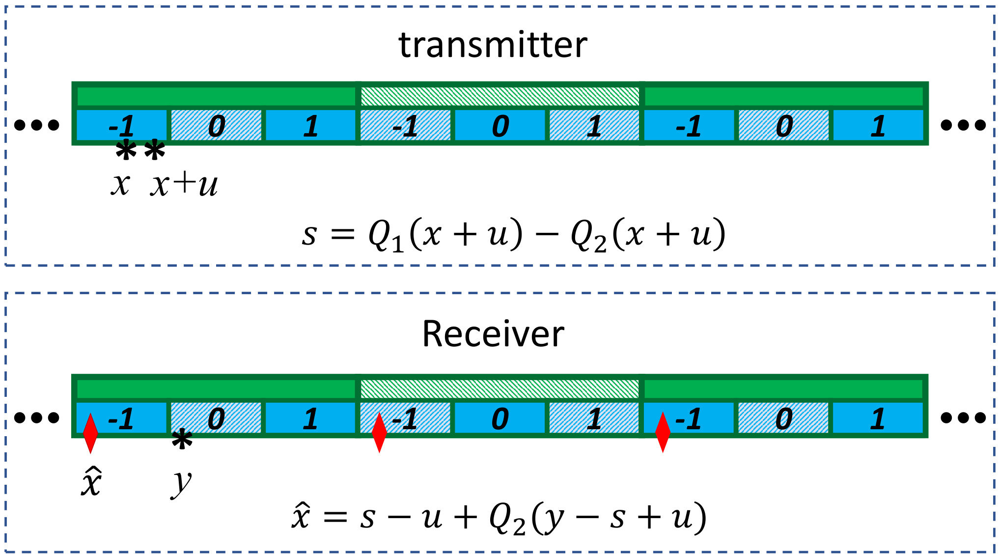
Figure 3 shows an example of using nested quantization, where $\Delta_{1}=1$ and $\Delta_{2}=3$. Let $x=-4.2$ and $u=0.3$ be the generated dither. Assume $\alpha=1$, hence $s=Q_{1}(-3.9)-Q_{2}(-3.9)=-4-(-3)=-1$ is the signal to be transmitted. Note that multiple points can produce the same $s$ with that dither signal, some are shown by $\blacklozenge$ in the figure, e.g., $-4.3.,-1.3,2.7,\ldots$ all leads to the same $s$. However, having access to $y=-3.4$ at the receiver can resolve the ambiguity. The value which resides in the same coarse quantization bin as $y$ is chosen, resulting in $\hat{x}=-4.3$. Note that in this nested quantization scheme, the output of quantizer is in $\{-1,0,+1\}$. If we wanted to achieve the same accuracy with a single quantizer, we had to transmit $s=-4$ instead of $s=-1$, increasing the number of bits depending on the range of $x$. For example, in Fig. 3, nested quantization reduces the range of quantization indexes from $\{-4,-3,\ldots,4\}$ to $\{-1,0,1\}$, reduction by a factor of $3$.

Our proposed distributed training using nested dithered quantization is summarized in Alg. 2 for one iteration of training ⁴⁴ 4 Note that we have ignored details on reproducing the pseudo-random sequences $\bm{u}_{k}$’s and updating seed numbers which are the same as in Alg. 1.. The stochastic gradient, computed by the $p$-th worker in a distributed training system, can be considered as a noisy estimate of the true gradient, i.e., $\bm{g}_{p}=\nabla_{\bm{w}}\mathcal{L}+\bm{\nu}_{p}$ where $\bm{\nu}_{p}$ is a zero-mean noise. However, as opposed to [14] and other similar works, the exact gradient $\nabla_{\bm{w}}\mathcal{L}$ is not available in distributed training. To overcome this issue, we propose to divide the workers into two groups. Set $\mathcal{P}_{1}$ of workers use DQSG with quantization step size $\Delta_{1}$, to provide an initial estimate for the true gradient. The parameter of the quantization and the number of workers in $\mathcal{P}_{1}$ are chosen such that the variance of averaged DQSG (see Lemma 3) becomes in an acceptable range, determined by Thm. 9. The workers in $\mathcal{P}_{2}$ use nested quantizer with step-sizes $(\Delta_{1}^{(p)},\Delta_{2}^{(p)})$ and scale $\alpha_{p}$. To decode the received Nested Dithered Quantized SG (NDQSG), the receiver uses the average of all SGs already received and decoded from other workers, denoted by $\overline{\widetilde{\bm{g}}}$. We assume that the SG of the $p$-th worker can be modeled as $\bm{g}_{p}=\overline{\widetilde{\bm{g}}}+\bm{z}_{p}$, where $\bm{z}_{p}$ is an independent random noise. Hence, the nested quantization uses $\overline{\widetilde{\bm{g}}}$ at the receiver as the side information to compute $\widetilde{\bm{g}}_{p}$. To find the quantization parameters, we can use the following result;

Note that setting $\alpha=1$ or $\alpha=\sqrt{1-\Delta_{1}^{2}/12\sigma_{z}^{2}}$ results in the same quantization variance as dithered quantization with step-size $\Delta_{1}$. However, nested quantization requires $\log_{2}(\Delta_{p_{2}}/\Delta_{p_{1}})$ bits to transmit each value, i.e., less than the ordinary quantization methods which requires almost $\log_{2}(2/\Delta_{p_{1}})$ bits.

References

- [1] F. Seide, H. Fu, J. Droppo, G. Li, and D. Yu, “1-bit stochastic gradient descent and its application to data-parallel distributed training of speech DNNs,” in Interspeech, 2014, pp. 1058–1062.
- [2] N. Dryden, S. A. Jacobs, T. Moon, and B. Van Essen, “Communication quantization for data-parallel training of deep neural networks,” in Proceedings of the Workshop on Machine Learning in High Performance Computing Environments, ser. MLHPC ’16. IEEE Press, 2016, pp. 1–8.
- [3] A. Øland and B. Raj, “Reducing communication overhead in distributed learning by an order of magnitude (almost),” in 2015 IEEE International Conference on Acoustics, Speech and Signal Processing (ICASSP), April 2015, pp. 2219–2223.
- [4] N. Strom, “Scalable distributed DNN training using commodity GPU cloud computing.” in INTERSPEECH, vol. 7, 2015, p. 10.
- [5] D. Alistarh, D. Grubic, J. Li, R. Tomioka, and M. Vojnovic, “Qsgd: Communication-efficient sgd via gradient quantization and encoding,” in Advances in Neural Information Processing Systems, 2017, pp. 1707–1718.
- [6] W. Wen, C. Xu, F. Yan, C. Wu, Y. Wang, Y. Chen, and H. Li, “Terngrad: Ternary gradients to reduce communication in distributed deep learning,” in Advances in Neural Information Processing Systems 30, I. Guyon, U. V. Luxburg, S. Bengio, H. Wallach, R. Fergus, S. Vishwanathan, and R. Garnett, Eds. Curran Associates, Inc., 2017, pp. 1509–1519.
- [7] J. Dean, G. Corrado, R. Monga, K. Chen, M. Devin, M. Mao, A. Senior, P. Tucker, K. Yang, Q. V. Le et al., “Large scale distributed deep networks,” in Advances in neural information processing systems, 2012, pp. 1223–1231.
- [8] F. Niu, B. Recht, C. Ré, and S. Wright, “Hogwild: A lock-free approach to parallelizing stochastic gradient descent,” in Advances in Neural Information Processing Systems 24, 2011, pp. 693–701.
- [9] H. Zhang, C. J. Hsieh, and V. Akella, “Hogwild++: A new mechanism for decentralized asynchronous stochastic gradient descent,” in 2016 IEEE 16th International Conference on Data Mining (ICDM), Dec 2016, pp. 629–638.
- [10] Q. Ho, J. Cipar, H. Cui, S. Lee, J. K. Kim, P. B. Gibbons, G. A. Gibson, G. Ganger, and E. Xing, “More effective distributed ML via a stale synchronous parallel parameter server,” in Advances in Neural Information Processing Systems 26, 2013, pp. 1223–1231.
- [11] L. Schuchman, “Dither signals and their effect on quantization noise,” IEEE Transactions on Communication Technology, vol. 12, no. 4, pp. 162–165, 1964.
- [12] R. M. Gray and T. G. Stockham, “Dithered quantizers,” IEEE Transactions on Information Theory, vol. 39, no. 3, pp. 805–812, 1993.
- [13] R. M. Gray and D. L. Neuhoff, “Quantization,” IEEE Transactions on Information Theory, vol. 44, no. 6, pp. 2325–2383, Oct 1998.
- [14] R. Zamir, S. Shamai, and U. Erez, “Nested linear/lattice codes for structured multiterminal binning,” IEEE Transactions on Information Theory, vol. 48, no. 6, pp. 1250–1276, Jun 2002.
- [15] R. Zamir, “Lattices are everywhere,” in 2009 Information Theory and Applications Workshop, Feb 2009, pp. 392–421.
- [16] A. Neelakantan, L. Vilnis, Q. V. Le, I. Sutskever, L. Kaiser, K. Kurach, and J. Martens, “Adding gradient noise improves learning for very deep networks,” arXiv preprint, 2015.
- [17] H. Noh, T. You, J. Mun, and B. Han, “Regularizing deep neural networks by noise: Its interpretation and optimization,” in Advances in Neural Information Processing Systems, 2017, pp. 5109–5118.
- [18] L. Bottou, “Online algorithms and stochastic approximations,” in Online Learning and Neural Networks, D. Saad, Ed. Cambridge, UK: Cambridge University Press, 1998, revised, oct 2012.
- [19] D. Slepian and J. Wolf, “Noiseless coding of correlated information sources,” IEEE Transactions on Information Theory, vol. 19, no. 4, pp. 471–480, July 1973.
- [20] Y. LeCun, L. Bottou, Y. Bengio, and P. Haffner, “Gradient-based learning applied to document recognition,” Proceedings of the IEEE, vol. 86, no. 11, pp. 2278–2324, 1998.
- [21] A. Krizhevsky, “One weird trick for parallelizing convolutional neural networks,” arXiv preprint arXiv:1404.5997, 2014.
- [22] S. Bubeck, “Convex optimization: Algorithms and complexity,” Foundations and Trends® in Machine Learning, vol. 8, no. 3-4, pp. 231–357, 2015.
Appendix A proof of Lemma 2
Let be a -level quantizer with step size . Let be the dither signal. Let be an arbitrary number. Assume that and define . Note that and
Similarly, . Comparing with stochastic quantizer, we see that they both assign the quantization points with the same probability. The case can be verified similarly.
Appendix B Proof of Lemma 3
To prove the unbiasedness, note that by Thm. 1, is independent from and uniformly distributed over . On the other hand, . Hence,
where (a) is due to the fact that is independent of and (b) because of unbiasedness of stochastic gradient and having mean zero.
For the variance,
where (c) follows from , and .
Appendix C A Note on Thm. 4
Because of the nature of quantization noise in our approach, the majority of convergence results with stochastic gradients can be readily applied to the DQSG. As an example, in this paper, we considered a result by [18]. To prove the convergence of (DQSGD), it suffices to show that there exists constants and such that ;
Therefore, for and , the DQSG is bounded and the theorem is proved following the same argument as in [18].
Appendix D A Note on Thm. 5
Appendix E Proof of Thm. 9
Let and . Then,
Since , it can be shown that
Therefore,
The correct decoding occurs when . Hence, the probability of correct recovery would be where
In that case,
Since and are independent from each other and from , simple calculations show that