跳到论文正文
W Papers独立论文阅读器 arXiv:1904.01190 论文正文 计算阅读时间 · 0%
引用这篇论文根据当前论文元数据生成,正式投稿前建议核对。


License: arXiv.org perpetual non-exclusive license
arXiv:1904.01190v2 [math.AP] 25 Aug 2019

Sharp Decay Estimates in Local Sensitivity Analysis for Evolution Equations with Uncertainties: from ODEs to Linear Kinetic Equations

Anton Arnold1    Shi Jin2    Tobias Wöhrer3 E-mail: anton.arnold@tuwien.ac.at E-mail: shijin-m@sjtu.edu.cn E-mail: tobias.woehrer@tuwien.ac.at
Abstract

We review the Lyapunov functional method for linear ODEs and give an explicit construction of such functionals that yields sharp decay estimates, including an extension to defective ODE systems. As an application, we consider three evolution equations, namely the linear convection-diffusion equation, the two velocity BGK model and the Fokker–Planck equation.

Adding an uncertainty parameter to the equations and analyzing its linear sensitivity leads to defective ODE systems. By applying the Lyapunov functional construction, we prove sharp long time behavior of order (1+tM)​e−μ​t(1+t^{M})e^{-\mu t}, where MM is the defect and μ\mu is the spectral gap of the system. The appearance of the uncertainty parameter in the three applications makes it important to have decay estimates that are uniform in the non-defective limit.

00footnotetext: The first author was partially supported by the FWF (Austrian Science Fund) funded SFB #F65. The first and the third authors were partially supported by the FWF-doctoral school W 1245 as well as the University of Madison-Wisconsin, where part of this work was carried out. The second author was partially supported by NSFC grants Nos. 31571071 and 11871297.
Keywords:
long time behavior, defective ODEs, kinetic equations, BGK models, Lyapunov functionals, uncertainty quantification, sensitivity analysis, non-defective limit, Fokker–Planck equations
††institute: Institute for Analysis and Scientific Computing, TU Vienna,
Wiedner Hauptstraße 8–10, 1040 Vienna, Austria,
,
website: https://www.asc.tuwien.ac.at/˜arnold/ and School of Mathematical Sciences, Institute of Natural Sciences, MOE-LSC, Shanghai Jiao Tong University,
Shanghai 200240, China,

and Institute for Analysis and Scientific Computing, TU Vienna,
Wiedner Hauptstraße 8–10, 1040 Vienna, Austria,

1 Introduction

Kinetic models arise from mesoscopic approximations of particle systems, as such, they are not first principle equations, thus contain empirical coefficients such as collision kernels in the Boltzmann equation, scattering coefficients in transport equations, forcing or source terms, and measurement errors in initial and boundary data, etc. Such errors can be modeled by uncertainties, or random inputs. Quantifying these uncertainties have important industrial and practical applications, in order to identify the sensitivities of input parameters, validate the models, conduct risk management, and ultimately improve these models.

In recent years one has seen activities in conducting uncertainty quantifications (UQ) for kinetic equations, see Hu2017 for a recent review. One of the important analysis in UQ is the so-called local sensitivity analysis, in which one aims to understand how sensitive the solution depends on the input parameters smithbook. For kinetic equations, a major tool to conduct sensitivity analysis for random kinetic equations has been the coercivity, or more generally, hypocoercivity, which originated in the study of long-time behavior of kinetic equations (see Villani-book; Dolbeault2015; MB; MN). In such analysis, by using the hypocoercivity of the kinetic operator, in a perturbative setting, namely, considering solutions near the global equilibrium (see Guo-NS), one can establish the long time convergence toward the local equilibrium with an exponential time decay rate. Such analysis has been extended to kinetic equations with random inputs, in both linear (see JLM; LiWang) and nonlinear (see JinZhu; LiuJin; ShuJin) settings. For stochastic Galerkin methods, hypocoercivity analysis even leads to exponential decay of numerical errors LiuJin; ShuJin, while in classical numerical analysis one often obtains errors that grow exponentially in time. In these works, however, the decay rates were not sharp.

Over the last two decades, entropy methods have become an important and robust tool to prove exponential convergence to equilibrium in kinetic and parabolic equations (see To; AMTU01; DeVi05; JuengelBook; Dolbeault2015). But sharpness of the decay rate is only known in few cases (see AMTU01 for the situation in Fokker–Planck equations). For linear finite dimensional ODEs, however, a method of constructing Lyapunov functionals to reveal optimal decay rates has been known for a long time, see Arnold1978, §22.4.

More recently in Arnold2014, such strategies were transferred to Fokker-Planck (FP) equations on ℝd\mathbb{R}^{d} and used to estimate the decay behavior of their solutions. For both, the ODE and the FP setting, one obtains the sharp exponential decay rate, as long as none of the eigenvalues determining the spectral gap of the generator is defective11 1 An eigenvalue is defective, if its algebraic multiplicity is strictly greater than its geometric multiplicity.. Recently this method was applied to PDEs that allow for a modal decomposition, like kinetic BGK models on the torus (see Achleitner2016; Achleitner2018). They are relaxation-type models for collisional gases, introduced by the physicists Bhatnagar, Gross and Krook in BGK.

In the defective case, however, the sharp decay behavior is of the form of a polynomial times an exponential, and different strategies have to be applied.

In order to catch the sharp decay behavior in the case of a defective FP equation, one can use the spectral properties of the FP operator to split the solution into two subspace-invariant parts: The first one corresponds to the spectral gap and is finite dimensional; there the sharp (defective) decay behavior can be computed explicitly. The second part of the solutions corresponds to a subspace “away” from the spectral gap, and it has a faster exponential decay. This approach gives sharp decay functions for defective FP equations for various entropies as shown in AEW17.

Alternatively, one can extend the Lyapunov functional by allowing it to be time dependent, see Monmarche2015. In §2 of this paper we will translate that strategy from linear Fokker–Planck equations in ℝd\mathbb{R}^{d} (as in Corollary 12 of Monmarche2015) to the ODE setting. We shall also refine the method such that it can yield uniform decay bounds in the non-defective limit. This extension will be crucial for our PDE-applications presented in §3–§5: a convection-diffusion equation, a BGK model and a linear Fokker–Planck equation on ℝ\mathbb{R} respectively. There we shall allow for uncertainty in the model coefficients and carry out a first (and for the convection-diffusion equations also second) order sensitivity analysis. In a local sensitivity analysis one tries to estimate the behavior of the (higher order) derivatives of the solution with respect to the input variables smithbook. Estimates of such derivatives are not only important to assess the sensitivity of the solution on the input parameters, they also provide regularity of the solution in the parameter space which is important to determine the convergence order of numerical approximations in the random space gunzburger2014stochastic; JLM; jin2017asymptotic. In the Fourier space, the resulting evolution equations for the parametric derivatives are mostly defective systems for which the sharp decay estimates can be obtained by using the Lyapunov functional approaches for defective deterministic systems. We would also like to point out that for the case of linear Fokker-Planck equation with a random drift, studied in §5, the global equilibrium is also random, while in previous sensitivity analysis for uncertain kinetic equations the global equilibria were all deterministic JinZhu; LiuJin.

2 Lyapunov functionals for defective ODEs

In this section we first review (from Achleitner2016) the Lyapunov functional method for non-defective ODEs and then extend it to the defective case. This is based on constructing a norm adapted to the problem that allows to recover the sharp decay behavior.

2.1 Construction of Lyapunov fuctionals

Let the matrix C∈ℂd×dC\in\mathbb{C}^{d\times d} be positive stable, i.e. its eigenvalues satisfy Re⁡(λi)>0\re(\lambda_{i})>0 for i=1,…,di=1,\ldots,d, and let μ:=mini=1,…,d⁡Re⁡(λi)>0\mu:=\min_{i=1,\ldots,d}\re(\lambda_{i})>0. We want to find a Lyapunov functional for the equation

dd​t​x​(t)=−C​x​(t),x∈ℂd,t≥0\displaystyle\frac{d}{dt}x(t)=-Cx(t),\quad x\in\mathbb{C}^{d},t\geq 0 (2.1)

that allows to deduce the sharp decay rate of solutions with energy-type estimates. For the construction of this functionals we consider the Jordan transformation of the matrix CHC^{H}, denoting the Hermitian transpose of the matrix CC (with eigenvalues λi¯\overline{\lambda_{i}}). We shall distinguish different cases of eigenvalue defectiveness:

CH=V​diag⁡(J1,…,JN)​V−1,\displaystyle C^{H}=V\operatorname{diag}(J_{1},\ldots,J_{N})V^{-1}, (2.2)

where JnJ_{n} for n∈{1,…,N}n\in\{1,\ldots,N\} are the Jordan blocks of CHC^{H} with length ln∈{1,…,d}l_{n}\in\{1,\ldots,d\}. A Jordan block of length one is an eigenvalue as a diagonal element, and a Jordan block JnJ_{n} of length ln>1l_{n}>1 corresponds to a chain of generalized eigenvectors of CHC^{H} of order kk satisfying

CH​vn(k)=λ¯n​vn(k)+vn(k−1),k∈{1,…,ln−1},\displaystyle C^{H}v_{n}^{(k)}=\overline{\lambda}_{n}v_{n}^{(k)}+v_{n}^{(k-1)},\quad k\in\{1,\ldots,l_{n}-1\}, (2.3)

where vn(0)v_{n}^{(0)} is an eigenvector of CHC^{H}, corresponding to λ¯n\overline{\lambda}_{n}. We denote the (semi-)
norm

|x|P2:=xH​P​x,|x|^{2}_{P}:=x^{H}Px,

for a Hermitian positive (semi-)definite matrix P∈ℂd×dP\in\mathbb{C}^{d\times d} to be defined.

Case 1: JnJ_{n} is a Jordan block of length ln=1l_{n}=1 with Re⁡(λn)≥μ\re(\lambda_{n})\geq\mu.

We define the rank 1 matrix22 2 For v,w∈ℂdv,w\in\mathbb{C}^{d} we denote v⊗w:=v⋅wHv\otimes w:=v\cdot w^{H} where ⋅\cdot is the matrix-matrix multiplication. Pn:=vn(0)⊗vn(0)P_{n}:=v_{n}^{(0)}\otimes v_{n}^{(0)} and get (cf. (2.51) in Arnold2014)

dd​t​|x⁡(t)|Pn2=−xH​(CH​Pn+Pn​C)​x≤−2​μ​xH​Pn​x=−2​μ|x⁡(t)|Pn2.\displaystyle\frac{d}{dt}|x(t)|^{2}_{P_{n}}=-x^{H}(C^{H}P_{n}+P_{n}C)x\leq-2\mu x^{H}P_{n}x=-2\mu|x(t)|_{P_{n}}^{2}. (2.4)

Case 2: JnJ_{n} is a Jordan block of length ln>1l_{n}>1 with Re⁡(λn)>μ\re(\lambda_{n})>\mu.

As in the proof of Lemma 4.3 in Arnold2014, we choose the coefficients bni>0b_{n}^{i}>0 as

bn1:=1;\displaystyle b_{n}^{1}:=1; bnj:=cj​(τn)2​(1−j),j∈{2,…,ln},\displaystyle b^{j}_{n}:=c_{j}(\tau_{n})^{2(1-j)},\quad j\in\{2,\ldots,l_{n}\},

where c1:=1c_{1}:=1, cj:=1+(cj−1)2c_{j}:=1+(c_{j-1})^{2} for j∈{2,…,ln}j\in\{2,\ldots,l_{n}\} and τn:=2​(Re⁡(λn)−μ)>0\tau_{n}:=2(\re(\lambda_{n})-\mu)>0. Then the matrix

Pn:=∑i=1lnbni​vn(i−1)⊗vn(i−1)\displaystyle P_{n}:=\sum_{i=1}^{l_{n}}b_{n}^{i}v_{n}^{(i-1)}\otimes v_{n}^{(i-1)}

satisfies

CH​Pn+Pn​C≥2​μ​Pn\displaystyle C^{H}P_{n}+P_{n}C\geq 2\mu P_{n} (2.5)

and, as in (2.4), one gets

dd​t​|x⁡(t)|Pn2≤−2​μ|x⁡(t)|Pn2.\displaystyle\frac{d}{dt}|x(t)|^{2}_{P_{n}}\leq-2\mu|x(t)|_{P_{n}}^{2}. (2.6)

Case 3: JnJ_{n} is a Jordan block of length ln>1l_{n}>1 with Re⁡(λn)=μ\re(\lambda_{n})=\mu.

A translation of the strategy of Corollary 12 in Monmarche2015 to the ODE setting leads to the following construction. For each m∈{1,…,ln}m\in\{1,\ldots,l_{n}\}, define the vector function

wnm​(t):=∑k=1mtm−k(m−k)!​vn(k−1),t≥0.\displaystyle w^{m}_{n}(t):=\sum^{m}_{k=1}\frac{t^{m-k}}{(m-k)!}v_{n}^{(k-1)},\quad t\geq 0. (2.7)

For m∈{2,…,ln}m\in\{2,\ldots,l_{n}\} we have

dd​t​wnm​(t)=∑k=1m−1tm−k−1(m−k−1)!​vn(k−1),\displaystyle\frac{d}{dt}w^{m}_{n}(t)=\sum^{m-1}_{k=1}\frac{t^{m-k-1}}{(m-k-1)!}v_{n}^{(k-1)},

from which it follows (using (2.3)) that

CH​wnm​(t)−λn¯​wnm​(t)=∑k=2mtm−k(m−k)!​vn(k−2)=dd​t​wnm​(t).\displaystyle C^{H}w^{m}_{n}(t)-\overline{\lambda_{n}}w^{m}_{n}(t)=\sum_{k=2}^{m}\frac{t^{m-k}}{(m-k)!}v_{n}^{(k-2)}=\frac{d}{dt}w^{m}_{n}(t). (2.8)

Next we define the time dependent Hermitian positive semi-definite matrix

Pnm​(t):=wnm​(t)⊗wnm​(t),m∈{1,…,ln}.\displaystyle P^{m}_{n}(t):=w^{m}_{n}(t)\otimes w^{m}_{n}(t),\quad m\in\{1,\ldots,l_{n}\}. (2.9)

Notice that wn1​(t)=vn(0)w^{1}_{n}(t)=v_{n}^{(0)}. So for m=1m=1 the computation for the estimate of dd​t​|x⁡(t)|Pn1​(t)2\frac{d}{dt}|x(t)|^{2}_{P^{1}_{n}(t)} is the same as in (2.4) (with equality since Re⁡(λn)=μ\re(\lambda_{n})=\mu). For m∈{2,…,ln}m\in\{2,\ldots,l_{n}\} we use the identity (2.8), and compute

dd​t​|x⁡(t)|Pnm​(t)2\displaystyle\frac{d}{dt}|x(t)|^{2}_{P^{m}_{n}(t)} =x˙H​(t)​Pnm​(t)​x​(t)+xH​(t)​Pnm​(t)​x˙​(t)+xH​(t)​Pnm˙​(t)​x​(t)\displaystyle=\dot{x}^{H}(t)P^{m}_{n}(t)x(t)+x^{H}(t)P^{m}_{n}(t)\dot{x}(t)+x^{H}(t)\dot{P^{m}_{n}}(t)x(t)
=−xH​(t)​[CH​wnm​(t)⊗wnm​(t)+wnm​(t)⊗wnm​(t)​C]​x​(t)\displaystyle=-x^{H}(t)[C^{H}w^{m}_{n}(t)\otimes w^{m}_{n}(t)+w^{m}_{n}(t)\otimes w^{m}_{n}(t)C]x(t)
+xH​(t)​[(CH​wnm​(t)−λn¯​wnm​(t))⊗wnm​(t)]​x​(t)\displaystyle\qquad+x^{H}(t)\left[(C^{H}w^{m}_{n}(t)-\overline{\lambda_{n}}w^{m}_{n}(t))\otimes w^{m}_{n}(t)\right]x(t)
+xH​(t)​[wnm​(t)⊗(CH​wnm​(t)−λn¯​wnm​(t))]​x​(t)\displaystyle\qquad+x^{H}(t)\left[w^{m}_{n}(t)\otimes(C^{H}w^{m}_{n}(t)-\overline{\lambda_{n}}w^{m}_{n}(t))\right]x(t)
=−2μxH(t)wnm(t)⊗wnm(t)x(t)=−2μ|x(t)|Pnm​(t)2\displaystyle=-2\mu x^{H}(t)w_{n}^{m}(t)\otimes w_{n}^{m}(t)x(t)=-2\mu|x(t)|^{2}_{P_{n}^{m}(t)}

and directly obtain

|x⁡(t)|Pnm​(t)2=e−2​μ​t​|x⁡(0)|Pnm​(0)2,t≥0.\displaystyle|x(t)|_{P^{m}_{n}(t)}^{2}=e^{-2\mu t}|x(0)|^{2}_{P^{m}_{n}(0)},\quad t\geq 0. (2.10)

For arbitrary βnm>0\beta_{n}^{m}>0, define

Pn​(t):=∑m=1lnβnm​Pnm​(t).\displaystyle P_{n}(t):=\sum^{l_{n}}_{m=1}\beta_{n}^{m}P^{m}_{n}(t). (2.11)

We have span⁡{vn(0),…,vn(ln−1)}=span⁡{wn1​(t),…,wnln​(t)}\linspan\{v_{n}^{(0)},\ldots,v_{n}^{(l_{n}-1)}\}=\linspan\{w^{1}_{n}(t),\ldots,w^{l_{n}}_{n}(t)\} for all t≥0t\geq 0, since the transformation matrix between these two sets is given by e−λn¯​t​eJn​te^{-\overline{\lambda_{n}}t}e^{J_{n}t}. Hence, the matrix Pn​(t)P_{n}(t) is positive definite on the subspace span⁡{vn(0),…,vn(ln−1)}\linspan\{v_{n}^{(0)},\ldots,v_{n}^{(l_{n}-1)}\}. In the corresponding semi-norm |⋅|Pn​(t)2|\cdot|_{P_{n}(t)}^{2} the solution x⁡(t)x(t) satisfies

|x⁡(t)|Pn​(t)2=e−2​μ​t​|x⁡(0)|Pn​(0)2,t≥0.\displaystyle|x(t)|^{2}_{P_{n}(t)}=e^{-2\mu t}|x(0)|^{2}_{P_{n}(0)},\quad t\geq 0.

For later convenience, we denote

Iμ:={n∈{1,…,N}∣ln>1,Re(λn)=μ},\displaystyle I_{\mu}:=\{n\in\{1,\ldots,N\}\mid l_{n}>1,\re(\lambda_{n})=\mu\}, (2.12)

to collect all indices with non-trivial Jordan blocks corresponding to μ\mu, i.e. corresponding to the above Case 3.

Combining the three cases:

Now let us define

P⁡(t)\displaystyle P(t) :=∑n∉Iμβn​Pn+∑n∈IμPn​(t)=∑n∉Iμβn​Pn+∑n∈Iμ∑m=1lnβnm​Pnm​(t),\displaystyle:=\sum_{n\not\in I_{\mu}}\beta_{n}P_{n}+\sum_{n\in I_{\mu}}P_{n}(t)=\sum_{n\not\in I_{\mu}}\beta_{n}P_{n}+\sum_{n\in I_{\mu}}\sum_{m=1}^{l_{n}}\beta_{n}^{m}P_{n}^{m}(t), (2.13)

where PnP_{n} and Pnm​(t)P_{n}^{m}(t) are chosen, depending on the above Cases 1–3 of the corresponding Jordan block JnJ_{n}. The weights βn>0\beta_{n}>0 are arbitrary in Cases 1–2, and the (arbitrary) βnm>0\beta_{n}^{m}>0 pertain to Case 3. The matrix P⁡(t)P(t) is positive definite for every t≥0t\geq 0, since it has full rank by construction and it is the sum of positive semi-definite matrices. It satisfies

dd​t​|x⁡(t)|P⁡(t)2≤−2​μ|x⁡(t)|P⁡(t)2,\displaystyle\frac{d}{dt}|x(t)|^{2}_{P(t)}\leq-2\mu|x(t)|^{2}_{P(t)}, (2.14)

and by applying Gronwall’s lemma, we conclude:

Lemma 1

Let C∈ℂd×dC\in\mathbb{C}^{d\times d} be positive stable and let μ>0\mu>0 be the smallest real part of all eigenvalues. Let diag⁡(J1,…,JN)\diag(J_{1},\ldots,J_{N}) be the Jordan normal form of CHC^{H}, where JnJ_{n} for n∈{1,…,N}n\in\{1,\ldots,N\} is a Jordan block of length lnl_{n} with eigenvalue λn¯\overline{\lambda_{n}}.

  1. 1.

    If all eigenvalues with real part equal to μ\mu are non-defective, i.e. Iμ=∅I_{\mu}=\emptyset, then there exists a time-independent Hermitian positive definite matrix P∈ℂd×dP\in\mathbb{C}^{d\times d}, such that the solutions to (2.1) satisfy

    |x⁡(t)|P2≤e−2​μ​t​|x⁡(0)|P2.\displaystyle|x(t)|^{2}_{P}\leq e^{-2\mu t}|x(0)|^{2}_{P}. (2.15)
  2. 2.

    If at least one eigenvalue with real part equal to μ\mu is defective, i.e. Iμ≠∅I_{\mu}\neq\emptyset, then there exists a time-dependent matrix P⁡(t)∈ℂd×dP(t)\in\mathbb{C}^{d\times d}, which is Hermitian positive definite for all t≥0t\geq 0 such that the solutions to (2.1) satisfy

    |x⁡(t)|P⁡(t)2≤e−2​μ​t​|x⁡(0)|P⁡(0)2.\displaystyle|x(t)|^{2}_{P(t)}\leq e^{-2\mu t}|x(0)|^{2}_{P(0)}. (2.16)

For further details on the algebraic interpretation of the time-independent matrix PP, we refer to the remarks following Lemma 4.3 in Arnold2014. See Example 2.2 in AAS (with ω≠0\omega\neq 0) for an ODE example and the relevance of the modified (time-independent) PP-norm for the trajectories of the ODE.

Remark 1

The matrix P⁡(t)P(t) is — with the construction described above — not unique. For one, arbitrary coefficients βn,βnm>0\beta_{n},\beta_{n}^{m}>0 in the definition of P⁡(t)P(t) in (2.13) are admissible. Secondly, the construction depends on the specific choice of (generalized) eigenvectors fixed in (2.3).

Remark 2

The matrix P⁡(t)P(t) can also be written as a matrix product:

P⁡(t)=V​eJ​t​Σ​(t)​B​(V​eJ​t)H,\displaystyle P(t)=Ve^{Jt}\Sigma(t)B(Ve^{Jt})^{H},

with VV and JJ from (2.2),

B:=diag⁡(β11,…,β1l1⏟l1​ entries,…,βN1,…,βNlN⏟lN​ entries)∈ℝd×d,\displaystyle B:=\diag(\underbrace{\beta_{1}^{1},\ldots,\beta_{1}^{l_{1}}}_{l_{1}\text{ entries}},\ldots,\underbrace{\beta_{N}^{1},\ldots,\beta_{N}^{l_{N}}}_{l_{N}\text{ entries}})\in\mathbb{R}^{d\times d},

with notation βnm:=βn\beta_{n}^{m}:=\beta_{n} for each n∉Iμn\not\in I_{\mu} and corresponding m∈{1,…,ln}m\in\{1,\ldots,l_{n}\} and

Σ⁡(t):=diag⁡(e−2​Re⁡(λ1)​t,…,e−2​Re⁡(λ1)​t⏟l1​ times,…,e−2​Re⁡(λN)​t,…,e−2​Re⁡(λN)​t⏟lN​ times)∈ℂd×d.\displaystyle\Sigma(t):=\diag(\underbrace{e^{-2\re(\lambda_{1})t},\ldots,e^{-2\re(\lambda_{1})t}}_{l_{1}\text{ times}},\ldots,\underbrace{e^{-2\re(\lambda_{N})t},\ldots,e^{-2\re(\lambda_{N})t}}_{l_{N}\text{ times}})\in\mathbb{C}^{d\times d}.

This representation of P⁡(t)P(t) directly implies that detP⁡(t)≡detP⁡(0)\det P(t)\equiv\det P(0) (cf. Fig. 3).

In the following remark and in Example 1, we investigate the geometry of the modified norms of Lemma 1.

Remark 3

For an ODE (2.1), we distinguish different eigenvalue settings of the matrix C∈ℂd×dC\in\mathbb{C}^{d\times d}, in order to isolate the interesting phenomena.

  • •

    Case 1: CC is in Case 1 of Lemma 1: Due to Lemma 1, there exists a time-independent PP-norm such that solutions decay as (2.15). The geometric reason for the strict decay is the following: This specific norm is modified such that the trajectories of solutions to the ODE are never tangential to the PP-norm level curves {x∈ℂd∣|x|P2=const.}\{x\in\mathbb{C}^{d}\mid|x|_{P}^{2}=\emph{const.}\} (cf. Fig. 2).

    To prove this, denote f⁡(x):=xH​P​xf(x):=x^{H}Px. Then, the normal vector of the PP-norm level curve at point x∈ℂd∖{0}x\in\mathbb{C}^{d}\setminus\{0\} is given as the PP-norm gradient of f⁡(x)f(x), i.e. η(x):=∇Pf(x)=P−1∇f(x)=2x\eta(x):=\nabla_{P}f(x)=P^{-1}\nabla f(x)=2x (see, e.g. (2.1.13) in jost for gradients of Riemannian manifolds). The (backwards-in-time facing) solution tangent vector at point xx is given as −x˙=C​x-\dot{x}=Cx. Due to the matrix inequality (2.5), η⁡(x)\eta(x) and −x˙-\dot{x} are never perpendicular, i.e. the PP-norm angle between them is bounded from below:

    ⟨x,C​x⟩P|x|P|​C​x|P\displaystyle\frac{\langle x,Cx\rangle_{P}}{|x|_{P}|Cx|_{P}} =xH​P​C​x|x|P|​C​x|P=12​xH​(CT​P+P​C)​x|x|P|​C​x|P\displaystyle=\frac{x^{H}PCx}{|x|_{P}|Cx|_{P}}=\frac{1}{2}\frac{x^{H}(C^{T}P+PC)x}{|x|_{P}|Cx|_{P}}
    ≥μ​xH​P​x|x|P|​C​x|P=μ​|x|P|C​x|P≥μ|C|P>0,\displaystyle\geq\mu\frac{x^{H}Px}{|x|_{P}|Cx|_{P}}=\mu\frac{|x|_{P}}{|Cx|_{P}}\geq\frac{\mu}{|C|_{P}}>0,

    where |C|P|C|_{P} denotes the matrix norm induced by the vector norm |x|P|x|_{P}.

  • •

    Case 2: CC is in Case 2 of Lemma 1: First, for the time-independent matrix PϵP_{\epsilon}, as defined in Arnold2014, Lemma 4.3, the analogous result as for the above case is true. The calculation is identical, up to replacing μ\mu by μ−ϵ\mu-\epsilon (cf. Example 1). Thus, also in the defective case, the solutions are never tangential to the level curves of the PϵP_{\epsilon}-norm.

    The P⁡(t)P(t)-norm of Case 2 in Lemma 1 has a different geometric effect on solutions due to its time-dependency. In fact, a solution x⁡(t)x(t) can even be tangential to the P⁡(t)P(t)-norm level curves for all times, while still maintaining sharp exponential decay, as Example 1 below shows.

  • •

    Case 3: All eigenvalues of CC have real part μ\mu (defective or non-defective): For t≥0t\geq 0, the P⁡(t)P(t)-angle between η⁡(x⁡(t))\eta(x(t)) and −x˙​(t)-\dot{x}(t) stays constant, i.e.

    ⟨x⁡(t),C​x​(t)⟩P⁡(t)|x⁡(t)|P⁡(t)|​C​x​(t)|P⁡(t)=⟨x⁡(0),C​x​(0)⟩P⁡(0)|x⁡(0)|P⁡(0)|​C​x​(0)|P⁡(0).\displaystyle\frac{\langle x(t),Cx(t)\rangle_{P(t)}}{|x(t)|_{P(t)}|Cx(t)|_{P(t)}}=\frac{\langle x(0),Cx(0)\rangle_{P(0)}}{|x(0)|_{P(0)}|Cx(0)|_{P(0)}}. (2.17)

    Indeed, in this case, (2.14) becomes an equality (with P⁡(t)≡P⁡(0)P(t)\equiv P(0), if all eigenvalues are non-defective), and hence |x⁡(t)|P⁡(t)2=e−2​μ​t​|x⁡(0)|P⁡(0)2|x(t)|_{P(t)}^{2}=e^{-2\mu t}|x(0)|_{P(0)}^{2} for all t≥0t\geq 0. In the following computation we use the polarization identity in the first and last step. The second identity follows from the fact that, if x⁡(t)x(t) is a solution to (2.1), so is (I+C)​x​(t)(I+C)x(t) and (I+i​C)​x​(t)(I+iC)x(t) (with initial conditions (I+C)​x​(0)(I+C)x(0) and (I+i​C)​x​(0)(I+iC)x(0), respectively):

    ⟨x⁡(t),C​x​(t)⟩P⁡(t)|x⁡(t)|P⁡(t)|​C​x​(t)|P⁡(t)=14​|x⁡(t)+C​x​(t)|P⁡(t)2−|​x​(t)−C​x​(t)|P⁡(t)2e−μ​t​|x⁡(0)|P⁡(0)​e−μ​t|​C​x​(0)|P⁡(0)\displaystyle\frac{\langle x(t),Cx(t)\rangle_{P(t)}}{|x(t)|_{P(t)}|Cx(t)|_{P(t)}}=\frac{1}{4}\frac{|x(t)+Cx(t)|_{P(t)}^{2}-|x(t)-Cx(t)|_{P(t)}^{2}}{e^{-\mu t}|x(0)|_{P(0)}e^{-\mu t}|Cx(0)|_{P(0)}}
    +14​i​|x⁡(t)−i​C​x​(t)|P⁡(t)2−i|​x​(t)+i​C​x​(t)|P⁡(t)2e−μ​t​|x⁡(0)|P⁡(0)​e−μ​t|​C​x​(0)|P⁡(0)\displaystyle\qquad\qquad+\frac{1}{4}\frac{i|x(t)-iCx(t)|_{P(t)}^{2}-i|x(t)+iCx(t)|_{P(t)}^{2}}{e^{-\mu t}|x(0)|_{P(0)}e^{-\mu t}|Cx(0)|_{P(0)}}
    =14​e−2​μ​t​|x⁡(0)+C​x​(0)|P⁡(0)2−e−2​μ​t|​x​(0)−C​x​(0)|P⁡(0)2e−μ​t​|x⁡(0)|P⁡(0)​e−μ​t|​C​x​(0)|P⁡(0)\displaystyle\qquad=\frac{1}{4}\frac{e^{-2\mu t}|x(0)+Cx(0)|_{P(0)}^{2}-e^{-2\mu t}|x(0)-Cx(0)|_{P(0)}^{2}}{e^{-\mu t}|x(0)|_{P(0)}e^{-\mu t}|Cx(0)|_{P(0)}}
    +14​e−2​μ​t​i​|x⁡(0)−i​C​x​(0)|P⁡(0)2−e−2​μ​t​i|​x​(0)+i​C​x​(0)|P⁡(0)2e−μ​t​|x⁡(0)|P⁡(0)​e−μ​t|​C​x​(0)|P⁡(0)\displaystyle\qquad\qquad+\frac{1}{4}\frac{e^{-2\mu t}i|x(0)-iCx(0)|_{P(0)}^{2}-e^{-2\mu t}i|x(0)+iCx(0)|_{P(0)}^{2}}{e^{-\mu t}|x(0)|_{P(0)}e^{-\mu t}|Cx(0)|_{P(0)}}
    =⟨x⁡(0),C​x​(0)⟩P⁡(0)|x⁡(0)|P⁡(0)|​C​x​(0)|P⁡(0)\displaystyle\qquad=\frac{\langle x(0),Cx(0)\rangle_{P(0)}}{|x(0)|_{P(0)}|Cx(0)|_{P(0)}}

    for all t≥0t\geq 0.

Example 1

Consider the IVP x˙=−C​x\dot{x}=-Cx, x⁡(0)=(6,6)Tx(0)=(6,6)^{T}, with matrix

C=(112−120),\displaystyle C=\begin{pmatrix}1&\frac{1}{2}\\ -\frac{1}{2}&0\end{pmatrix},

which has the defective eigenvalue and spectral gap λ=μ=12\lambda=\mu=\frac{1}{2} and the (generalized) eigenvectors

w(0)=12​(1,−1)T,\displaystyle w^{(0)}=\frac{1}{\sqrt{2}}\begin{pmatrix}1,&-1\end{pmatrix}^{T}, w(1)=12​(1,1)T.\displaystyle w^{(1)}=\frac{1}{\sqrt{2}}\begin{pmatrix}1,&1\end{pmatrix}^{T}.

Our goal is to obtain a better geometric understanding of the necessity of a time-dependent norm for sharp decay estimates of solutions. To this end, we compare the here presented Lyapunov functional constructions with functionals considered in Arnold2014.

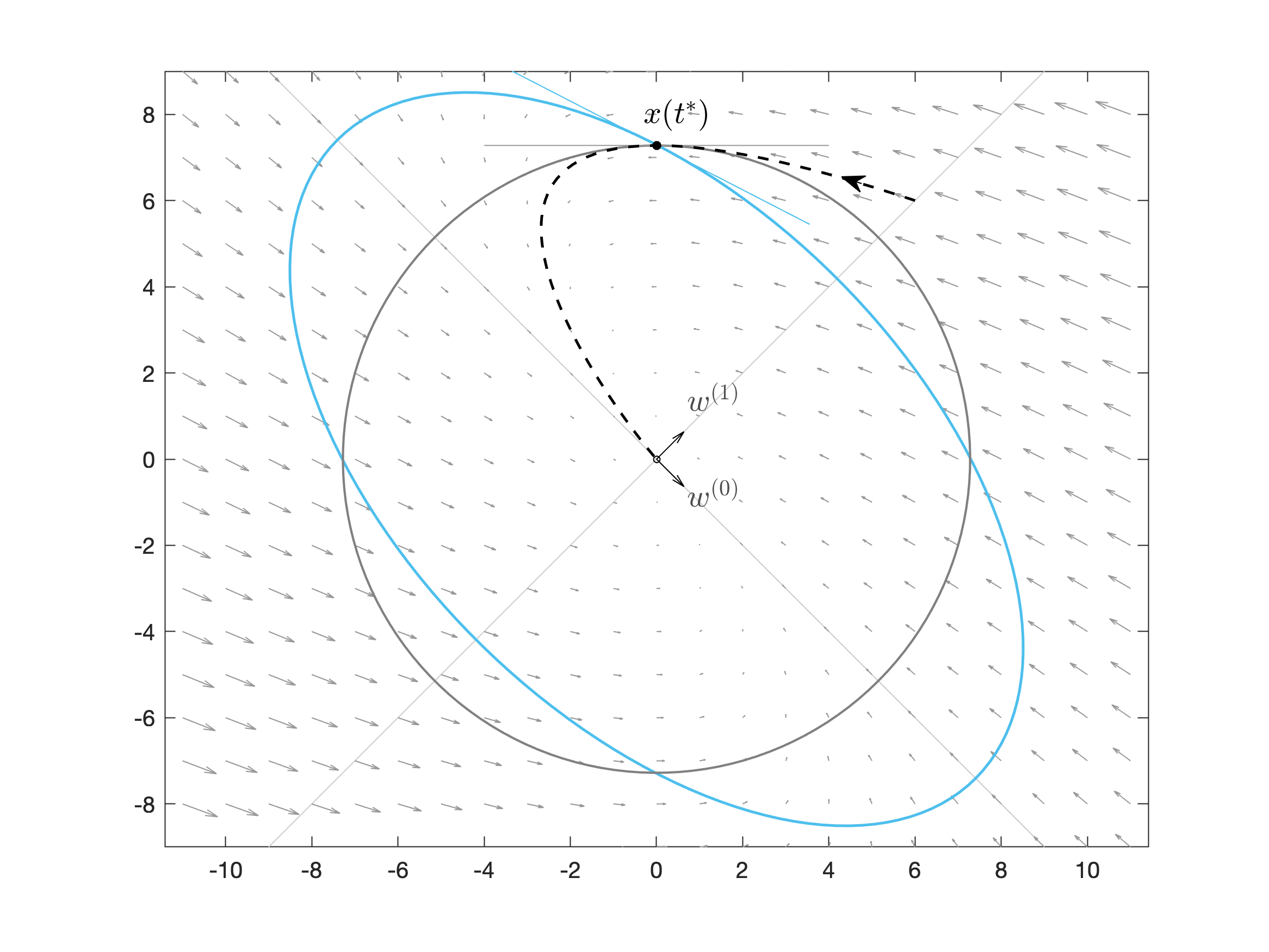
The naive approach of using the Euclidean norm of the solution x⁡(t)x(t) exhibits non strict decay (the dashed curve in Fig. 1 has a horizontal tangent at t=1t=1). The time-independent norm |⋅|Pϵ|\cdot|_{P_{\epsilon}}, as defined in Arnold2014, Lemma 4.3, with the matrix

Pϵ=12​(12​ϵ2+112​ϵ2−112​ϵ2−112​ϵ2+1),ϵ>0,\displaystyle P_{\epsilon}=\frac{1}{\sqrt{2}}\begin{pmatrix}\frac{1}{2\epsilon^{2}}+1&\frac{1}{2\epsilon^{2}}-1\\ \frac{1}{2\epsilon^{2}}-1&\frac{1}{2\epsilon^{2}}+1\end{pmatrix},\quad\epsilon>0,

yields uniform exponential decay, but the rate μ−ϵ\mu-\epsilon is not sharp. See Fig. 1 for the decay plot and Fig. 2 for a geometric reasoning why a modified norm can yield exponential decay.

The P⁡(t)P(t)-norm, with matrix

P⁡(t)=12​(t2+2​t+2t2t2t2−2​t+2),\displaystyle P(t)=\frac{1}{2}\begin{pmatrix}t^{2}+2t+2&t^{2}\\ t^{2}&t^{2}-2t+2\end{pmatrix},

as defined in (2.13) (with weights β1=β2=1\beta^{1}=\beta^{2}=1), provides the sharp exponential decay

|x⁡(t)|P⁡(t)2=e−t​|x⁡(0)|P⁡(0)2=e−t​|x⁡(0)|22,t≥0.|x(t)|_{P(t)}^{2}=e^{-t}|x(0)|_{P(0)}^{2}=e^{-t}|x(0)|^{2}_{2},\qquad t\geq 0.

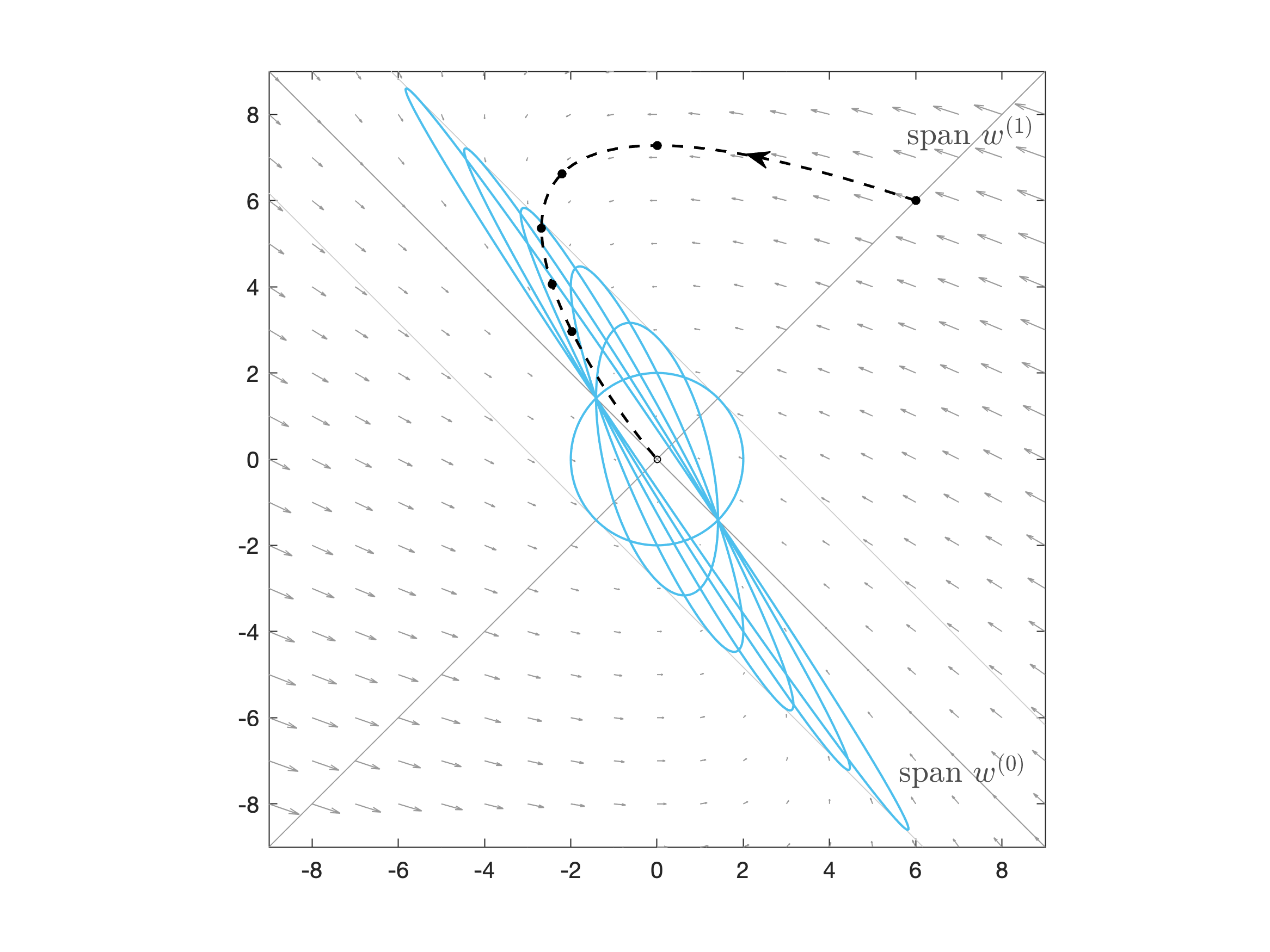
See Figures 3–4 for the geometric evolution of the P⁡(t)P(t)-norm.

Choosing the initial condition x~​(0)=(0,7)T\tilde{x}(0)=(0,7)^{T}, yields the solution x~​(t)\tilde{x}(t) that is tangential to the P⁡(t)P(t)-norm level curve for each t≥0t\geq 0, while the exponential decay of the solution in P⁡(t)P(t)-norm is still sharp, see Figure 5.

◇\Diamond

Refer to caption
Figure 1: The dashed line shows the decay of the solution in the Euclidean norm. It initially exhibits a wavy behavior, where at time t∗=1t^{*}=1, there is no strict decay at all. The dotted line describes the solution in PϵP_{\epsilon}-norm with ϵ=0.4\epsilon=0.4. It yields uniform exponential decay, however, the decay rate is not sharp. The solid line shows the decay of |x⁡(t)|P⁡(t)|x(t)|_{P(t)} with sharp exponential rate e−12​te^{-\frac{1}{2}t}.
Refer to caption
Figure 2: The dashed line shows the solution trajectory x⁡(t)x(t). At the marked point x⁡(t∗)x(t^{*}), the solution is tangential to the Euclidean level curve. This implies non-strict decay in the Euclidean norm (cp. Fig. 1) at t∗=1t^{*}=1. The ellipse represents a level curve of the PϵP_{\epsilon}-norm (with ϵ=0.4\epsilon=0.4). It modifies the geometry such that the solution is never tangential to the level curves of |⋅|Pϵ|\cdot|_{P_{\epsilon}}. This assures strict exponential decay in the PϵP_{\epsilon}-norm, however the rate is not sharp.
Refer to caption
Figure 3: The dashed line in the plot describes the solution x⁡(t)x(t) with the marked points x⁡(0),x⁡(1),…,x⁡(5)x(0),x(1),\ldots,x(5). Additionally, the level curves of {x∈ℝ2∣|x|P⁡(t)2=4}\{x\in\mathbb{R}^{2}\mid|x|_{P(t)}^{2}=4\} for t=0,1,…,5t=0,1,\ldots,5 are plotted. In direction of the eigenvector of the matrix CC, w(0)w^{(0)}, the distances stay constant in time. The area spanned by each ellipse-shaped level curve stays constant (cf. Remark 2), while the semi-major axis of the ellipse stretches out and tilts towards the eigenvector axis w(0)w^{(0)} as time increases. The stretch is linear in tt in the direction of ±w(0)\pm w^{(0)}: For arbitrary t≥0t\geq 0, the point ±2​(1−t,1+t)T\pm\sqrt{2}(1-t,1+t)^{T} is on the ellipse with the tangent (±2,±2)T+span⁡{w(0)}(\pm\sqrt{2},\pm\sqrt{2})^{T}+\linspan\{w^{(0)}\}.
Refer to caption
Figure 4: The level curves of {x∈ℝ2∣|x|P⁡(t)2=e−t​|x⁡(0)|22}\{x\in\mathbb{R}^{2}\mid|x|_{P(t)}^{2}=e^{-t}|x(0)|^{2}_{2}\} for t=0,1,…,4t=0,1,\ldots,4 are plotted (cp. Fig. 3). They intersect with the solution trajectories exactly at the marked points x⁡(0),x⁡(1),…,x⁡(4)x(0),x(1),\ldots,x(4), which corresponds to the statement of Lemma 1, Case 2. Notice that the tangents of the level curves of |⋅|P⁡(t)|\cdot|_{P(t)} at x⁡(t)x(t) are all parallel to each other. The intersection angle in the P⁡(t)P(t)-norm is time-independent, see Remark 3, Case 3.
Refer to caption
Figure 5: The level curves of {x∈ℝ2∣|x|P⁡(t)2=e−t​|x~​(0)|22}\{x\in\mathbb{R}^{2}\mid|x|_{P(t)}^{2}=e^{-t}|\tilde{x}(0)|^{2}_{2}\} for t=0,1,…,4t=0,1,\ldots,4 are plotted analogous to Fig. 4, but here for the initial value x~​(0)=(0,7)T\tilde{x}(0)=(0,7)^{T}. The solution x~​(t)\tilde{x}(t) is tangential to the P⁡(t)P(t)-norm level curves for each t≥0t\geq 0.

Lemma 1 shows that the P⁡(t)P(t)-norm of any solution to (2.1) decays exponentially. But due to the time dependence of the norm itself, it is not evident that this is an appropriate functional to capture the sharp decay rate of solutions. Hence, we shall next compare the P⁡(t)P(t)-norm to the Euclidean norm.

An arbitrary Hermitian positive definite matrix P∈ℂn×nP\in\mathbb{C}^{n\times n} satisfies

λminP​I≤P≤λmaxP​I,\displaystyle\lambda^{P}_{\min}I\leq P\leq\lambda^{P}_{\max}I, (2.18)

where λminP\lambda_{\min}^{P} is the smallest and λmaxP\lambda_{\max}^{P} is the largest eigenvalue of PP. Using this inequality for P⁡(t)P(t), and the decay estimate (2.16), leads to the Euclidean decay estimate

|x⁡(t)|22\displaystyle|x(t)|^{2}_{2} ≤(λminP⁡(t))−1​|x⁡(t)|P⁡(t)2≤(λminP⁡(t))−1​e−2​μ​t|x⁡(0)|P⁡(0)2\displaystyle\leq(\lambda_{\min}^{P(t)})^{-1}|x(t)|_{P(t)}^{2}\leq(\lambda_{\min}^{P(t)})^{-1}e^{-2\mu t}|x(0)|_{P(0)}^{2}
≤(λminP⁡(t))−1​λmaxP⁡(0)​e−2​μ​t​|x⁡(0)|22.\displaystyle\leq(\lambda_{\min}^{P(t)})^{-1}\lambda^{P(0)}_{\max}e^{-2\mu t}|x(0)|_{2}^{2}.

But here the decay behavior is “hidden” in the smallest eigenvalue of P⁡(t)P(t). The true qualitative behavior of |x⁡(t)|22|x(t)|_{2}^{2} will be derived next.

The following technical Lemma 2 allows us, in the subsequent step, to estimate the time-dependency of the Pnm​(t)P_{n}^{m}(t)-semi-norm. The strategy of the proof has already been used for Corollary 12 of Monmarche2015 in the setting of Fokker–Planck equations on ℝd\mathbb{R}^{d}. However, our refined estimate here, for one, provides an upper bound for the time-dependence of a more general class of modified norms. And additionally, the constants appearing in the estimate are explicit, depending on mm and a parameter θ\theta which, later on, allows to optimize the constants in the decay estimate of solutions to the ODE (2.1).

Lemma 2

For linearly independent vectors v1,…,vm∈ℂdv^{1},\ldots,v^{m}\in\mathbb{C}^{d} define

w^m​(t):\displaystyle\hat{w}^{m}(t): =ξm​vm+∑j=1m−1ξj​(t)​vj,\displaystyle=\xi^{m}v^{m}+\sum_{j=1}^{m-1}\xi^{j}(t)v^{j}, (2.19)

where ξj​(t)\xi^{j}(t) for j∈{1,…,m−1}j\in\{1,\ldots,m-1\} are (arbitrary) real-valued polynomials in t≥0t\geq 0, and ξm>0\xi^{m}>0. Furthermore let

P^m​(t):=w^m​(t)⊗w^m​(t),t≥0;Qj:=vj⊗vj,j∈{1,…,m}.\displaystyle\hat{P}^{m}(t):=\hat{w}^{m}(t)\otimes\hat{w}^{m}(t),\quad t\geq 0;\qquad Q^{j}:=v^{j}\otimes v^{j},\quad j\in\{1,\ldots,m\}.

Then, the following inequality holds for every x∈ℂdx\in\mathbb{C}^{d}, θ∈(0,1)\theta\in(0,1) and t≥0:t\geq 0:

|x|P^m​(t)2≥(1−θ)​(ξm)2​|x|Qm2−((m−1)2θ−1)​∑k=1m−1(ξk​(t))2|​x|Qk2.\displaystyle|x|_{\hat{P}^{m}(t)}^{2}\geq(1-\theta)(\xi^{m})^{2}|x|^{2}_{Q^{m}}-\left(\frac{(m-1)^{2}}{\theta}-1\right)\sum_{k=1}^{m-1}(\xi^{k}(t))^{2}|x|^{2}_{Q^{k}}.

Notice that the second (tt-dependent) term of the r.h.s. involves only the semi-norms |x|Q1,…,|x|Qm−1|x|_{Q^{1}},\ldots,|x|_{Q^{m-1}}.

The technical proof is deferred to Appendix A.1.

Remark 4

Lemma 2 is formulated in a general form, to be applicable also to §4 below. Here, we use it to estimate the time-dependency of the Pnm​(t)P_{n}^{m}(t)-semi-norms (as defined in (2.9)) for arbitrary n∈Iμn\in I_{\mu} and corresponding m∈{2,…,ln}m\in\{2,\ldots,l_{n}\}. In notation of Lemma 2, choose v1=vn(0),…,vm=vn(m−1)v^{1}=v_{n}^{(0)},\ldots,v^{m}=v_{n}^{(m-1)} and ξk​(t)=tm−k(m−k)!\xi^{k}(t)=\frac{t^{m-k}}{(m-k)!} for k∈{1,…,m}k\in\{1,\ldots,m\}, which leads to w^nm​(t)=wnm​(t)\hat{w}_{n}^{m}(t)=w_{n}^{m}(t). Then, Lemma 2 yields

|x|Pnm​(t)2≥(1−θ)​|x|Pnm​(0)2−((m−1)2θ−1)​∑k=1m−1(tm−k(m−k)!)2|​x|Pnk​(0)2,\displaystyle\begin{aligned} &\qquad|x|_{P_{n}^{m}(t)}^{2}\geq\\ &\qquad\quad\left(1-\theta\right)|x|^{2}_{P_{n}^{m}(0)}-\left(\frac{(m-1)^{2}}{\theta}-1\right)\sum^{m-1}_{k=1}\left(\frac{t^{m-k}}{(m-k)!}\right)^{2}|x|^{2}_{P_{n}^{k}(0)},\end{aligned} (2.20)

for every n∈Iμn\in I_{\mu}, all corresponding m∈{2,…,ln}m\in\{2,\ldots,l_{n}\}, x∈ℂdx\in\mathbb{C}^{d}, θ∈(0,1)\theta\in(0,1) and t≥0t\geq 0.

In the next step, we combine the exponential decay in P⁡(t)P(t)-norm of solutions, (2.16) with the lower bound (2.20). This allows to estimate the P⁡(0)P(0)-norm decay of solutions and, consequently, the decay behavior in the Euclidean norm. In contrast to the result stated in Monmarche2015 for the FP setting, we obtain an multiplicative constant 𝒞\mathscr{C} in the estimate depending explicitly on the maximal defect associated to μ\mu and the choice of the weights βnm\beta_{n}^{m} of P⁡(t)P(t).

The freedom of choice in the weights and their influence on the constant 𝒞\mathscr{C} is of great importance in §3–§5, as 𝒞\mathscr{C} will need to stay bounded in the non-defective limit (see Example 2 below).

Theorem 2.1

Let C∈ℂd×dC\in\mathbb{C}^{d\times d} be positive stable and let μ>0\mu>0 be the smallest real part of all eigenvalues. Let MM be the maximal size of a Jordan block associated to μ\mu (i.e. the maximal defect associated to μ\mu is M−1M-1). Then there exists a constant 𝒞>0\mathscr{C}>0, such that the solutions to (2.1) satisfy

|x⁡(t)|22≤𝒞⁡(1+t2​(M−1))​e−2​μ​t​|x⁡(0)|22.\displaystyle|x(t)|^{2}_{2}\leq\mathscr{C}(1+t^{2(M-1)})e^{-2\mu t}|x(0)|_{2}^{2}. (2.21)

The constant 𝒞\mathscr{C} can be chosen as

𝒞:={(λminP)−1​λmaxP,M=1,2​(λminP⁡(0))−1​λmaxP⁡(0)​cM​maxn∈Iμ​[∑m=1lnβnmmink∈{1,…,m}⁡βnk],M≥2,\displaystyle\mathscr{C}:=\begin{cases}(\lambda_{\min}^{P})^{-1}\lambda_{\max}^{P},&M=1,\\ 2(\lambda_{\min}^{P(0)})^{-1}\lambda_{\max}^{P(0)}c_{M}\,\displaystyle\max_{n\in I_{\mu}}\Big[\sum_{m=1}^{l_{n}}\frac{\beta_{n}^{m}}{\displaystyle\min_{k\in\{1,\ldots,m\}}\beta_{n}^{k}}\Big],&M\geq 2,\end{cases} (2.22)

where λminP⁡(0)\lambda_{\min}^{P(0)} is the smallest and λmaxP⁡(0)\lambda_{\max}^{P(0)} is the largest eigenvalue of the matrix P⁡(0)P(0) (with P⁡(0)≡PP(0)\equiv P for M=1M=1), which is defined in (2.13). The constants cMc_{M} for M≥2M\geq 2 are given as:

cM\displaystyle c_{M} =2M−2​(∏j=1M−14​j2−1)​(∏j=2M∑k=1j1[(j−k)!]2).\displaystyle=2^{M-2}\left(\prod_{j=1}^{M-1}4j^{2}-1\right)\left(\prod_{j=2}^{M}\sum_{k=1}^{j}\frac{1}{[(j-k)!]^{2}}\right).

The technical proof of this result is deferred to Appendix A.2.

Remark 5

If, for all n∈Iμn\in I_{\mu}, the weights βnm\beta_{n}^{m} of the matrix P⁡(0)P(0) are monotonically decreasing in mm, i.e. βnm≥βnm+1\beta_{n}^{m}\geq\beta_{n}^{m+1} for m∈{1,…,ln−1}m\in\{1,\ldots,l_{n}-1\}, then

maxn∈Iμ⁡[∑m=1lnβnmmink∈{1,…,m}⁡βnk]=M.\displaystyle\displaystyle\max_{n\in I_{\mu}}\Big[\sum_{m=1}^{l_{n}}\frac{\beta_{n}^{m}}{\displaystyle\min_{k\in\{1,\ldots,m\}}\beta_{n}^{k}}\Big]=M.
Remark 6

Note that we could calculate the solution to the ODE system (2.1) directly, by means of its Jordan transformation, and get qualitatively the same decay behavior as in (2.21), but possibly with a different multiplicative constant: Using x⁡(t)=e−C​t​x​(0)x(t)=e^{-Ct}x(0), C=(VH)−1​JH​VHC=(V^{H})^{-1}J^{H}V^{H}, we obtain

|x⁡(t)|22\displaystyle|x(t)|_{2}^{2} ≤|V|22​|V−1|22|​e−JH​t|22|x⁡(0)|22\displaystyle\leq|V|^{2}_{2}|V^{-1}|^{2}_{2}|e^{-J^{H}t}|^{2}_{2}|x(0)|^{2}_{2}
≤|V|22|​V−1|22​c^M​(1+t2​(M−1))​e−2​μ​t|x⁡(0)|22,\displaystyle\leq|V|^{2}_{2}|V^{-1}|^{2}_{2}\hat{c}_{M}(1+t^{2(M-1)})e^{-2\mu t}|x(0)|^{2}_{2}, (2.23)

where |V|2|V|_{2} denotes the matrix norm induced by the vector norm |⋅|2|\cdot|_{2}, VV is the transformation matrix from (2.2), J:=diag⁡(J1,…,JN)J:=\diag(J_{1},\ldots,J_{N}) the corresponding Jordan matrix, and c^M\hat{c}_{M} depends only on the largest Jordan block. So what is the gain of the result in Theorem 2.1?

Firstly, the construction of the matrix P⁡(t)P(t) and the method of estimating the P⁡(t)P(t)-norm decay of the solution can be translated almost directly to the infinite dimensional setting of the Fokker–Planck equation with linear drift, where a direct way of calculating the decay (as in the finite dimensional ODE case) is not possible (see Arnold2014 for the exponential decay in the non-defective case and Monmarche2015 for an improved decay in the defective case). In the Fokker–Planck setting on ℝd\mathbb{R}^{d}, the place of the P⁡(t)P(t)-norm is taken by the modified Fisher information involving P⁡(t)P(t).

Secondly, the result also makes it possible to systematically calculate the multiplicative constant 𝒞\mathscr{C} from (2.21), which we will use in §3–§5, and which can be further exploited to get decay results for infinite dimensional ODE systems (see Achleitner2016, §4.3).

2.2 Uniform decay estimates in non-defective limits

The advantage of the P⁡(t)P(t)-norm estimation compared to (2.23) can be seen in the following example.

Example 2

Consider the matrix

Cϵ:=(1ϵ01)\displaystyle C_{\epsilon}:=\begin{pmatrix}1\penalty\ &\epsilon\\ 0\penalty\ &1\end{pmatrix}

with arbitrary ϵ≠0\epsilon\neq 0. Its corresponding Jordan transformation matrix reads

Vϵ:=(1001ϵ),\displaystyle V_{\epsilon}:=\begin{pmatrix}1\penalty\ &0\\ 0\penalty\ &\frac{1}{\epsilon}\end{pmatrix},

and M=2M=2. For ϵ→0\epsilon\to 0 the factor |Vϵ|2|​Vϵ−1|2|V_{\epsilon}|_{2}|V_{\epsilon}^{-1}|_{2} in (2.23) becomes unbounded of order ϵ−2\epsilon^{-2} (even though the true decay of the solution improves to e−t​|x⁡(0)|2e^{-t}|x(0)|_{2} in the limit). This is due to the discontinuity of the Jordan transformation at the transition from defectiveness to non-defectiveness. We apply Theorem 2.1 to the ODE system x˙=−Cϵ​x\dot{x}=-C_{\epsilon}x, with the following eigenvectors of CϵHC_{\epsilon}^{H}:

v1(0)=(0,1)T and v1(1)=(1ϵ,0)T.\displaystyle v^{(0)}_{1}=\begin{pmatrix}0,&1\end{pmatrix}^{T}\quad\text{ and }\quad v^{(1)}_{1}=\begin{pmatrix}\frac{1}{\epsilon},&0\end{pmatrix}^{T}.

When using β1,ϵ1=1\beta_{1,\epsilon}^{1}=1 and β1,ϵ2=ϵ2\beta_{1,\epsilon}^{2}=\epsilon^{2} in (2.13), we get Pϵ​(0)=IP_{\epsilon}(0)=I, and hence the constant

𝒞ϵ=12⋅max⁡{2,1+ϵ2}\displaystyle\mathscr{C}_{\epsilon}=12\cdot\max\{2,1+\epsilon^{2}\} (2.24)

stays bounded in the non-defective limit ϵ→0\epsilon\to 0. ◇\Diamond

This example shows that, while the method presented here is still relying on the Jordan transformation (as P⁡(t)P(t) is constructed with generalized eigenvectors), the additional weights βnm\beta_{n}^{m} in the matrix P⁡(t)P(t) allow for estimates more closely related to the actual behavior of the solutions. As sketched in Example 2 this can allow for (but does not guarantee) an estimate that is uniform in the non-defective limit. In §3–§5 we will see further examples of specific choices of the weights βnm\beta_{n}^{m} that lead to uniform estimates in the non-defective limit.

Remark 7

While the proof of Theorem 2.1 is formulated to work for arbitrarily large defects, more careful estimations can improve the decay estimate. We shall now show an improvement for defect one. For any n∈Iμn\in I_{\mu} the inequality (A.2) with m=2m=2 and θ=12\theta=\frac{1}{2} yields

|x⁡(t)|Pn2​(0)2≤2​e−2​μ​t​(t2​|x⁡(0)|Pn1​(0)2+|x⁡(0)|Pn2​(0)2),\displaystyle|x(t)|_{P_{n}^{2}(0)}^{2}\leq 2e^{-2\mu t}\left(t^{2}|x(0)|^{2}_{P_{n}^{1}(0)}+|x(0)|_{P_{n}^{2}(0)}^{2}\right),

where we used (2.10) with Pn1​(t)=Pn1​(0)P_{n}^{1}(t)=P_{n}^{1}(0).

For n∈Iμn\in I_{\mu} with ln=2l_{n}=2 the decay estimate for Pn​(0)=βn1​Pn1​(0)+βn2​Pn2​(0)P_{n}(0)=\beta^{1}_{n}P^{1}_{n}(0)+\beta^{2}_{n}P^{2}_{n}(0) follows as

|x⁡(t)|Pn​(0)2≤2​e−2​μ​t​(1+βn2βn1​t2)​|x⁡(0)|Pn​(0)2.\displaystyle|x(t)|^{2}_{P_{n}(0)}\leq 2e^{-2\mu t}(1+\frac{\beta_{n}^{2}}{\beta^{1}_{n}}t^{2})|x(0)|^{2}_{P_{n}(0)}.

We can use this estimate to get an improved upper bound for solutions from Example 2 in the Euclidean norm (compared to (2.21) with (2.24)): With the same matrix choice Pϵ​(0)=P11​(0)+ϵ2​P12​(0)=IP_{\epsilon}(0)=P^{1}_{1}(0)+\epsilon^{2}P^{2}_{1}(0)=I as in Example 2, it follows that solutions to x˙=−Cϵ​x\dot{x}=-C_{\epsilon}x satisfy

|x⁡(t)|22\displaystyle|x(t)|_{2}^{2} =|x⁡(t)|Pϵ​(0)2≤2​e−2​t​(1+ϵ2​t2)​|x⁡(0)|22,t≥0.\displaystyle=|x(t)|_{P_{\epsilon}(0)}^{2}\leq 2e^{-2t}(1+\epsilon^{2}t^{2})|x(0)|^{2}_{2},\quad t\geq 0. (2.25)

This estimate not only yields a bounded multiplicative constant for ϵ→0\epsilon\to 0, but also yields a sharp decay rate — namely purely exponential — for the non-defective limit case ϵ=0\epsilon=0. In comparison, the solution propagator norm estimate for all ϵ∈ℝ\epsilon\in\mathbb{R} is given as

|e−Cϵ​t​x​(0)|22\displaystyle|e^{-C_{\epsilon}t}x(0)|_{2}^{2} =e−2​t​|(1−ϵ​t0 1)|22​|x⁡(0)|22\displaystyle=e^{-2t}\left|\begin{pmatrix}1&-\epsilon t\\ 0&\penalty\ 1\end{pmatrix}\right|^{2}_{2}|x(0)|^{2}_{2}
=e−2​t​(1+ϵ2​t22+ϵ2​t2+ϵ4​t44)​|x⁡(0)|22\displaystyle=e^{-2t}\left(1+\frac{\epsilon^{2}t^{2}}{2}+\sqrt{\epsilon^{2}t^{2}+\frac{\epsilon^{4}t^{4}}{4}}\right)|x(0)|^{2}_{2} (2.26)
≈ϵ​t→∞​e−2​t​(2+ϵ2​t2)​|x⁡(0)|22.\displaystyle\overset{\epsilon t\to\infty}{\approx}e^{-2t}(2+\epsilon^{2}t^{2})|x(0)|^{2}_{2}.

This shows that (2.25) is rather accurate.

Remark 8

Consider an ODE (2.1) with matrix CC that has a Jordan block Jn2J_{n_{2}} in Case 2 from §2.1, i.e. ln2>1l_{n_{2}}>1 and Re⁡(λn2)>μ\re(\lambda_{n_{2}})>\mu. Then, the construction of Case 2 can be replaced with the one of Case 3. This means, exchanging the time-constant matrix Pn2P_{n_{2}}, which has predetermined weights bn2mb_{n_{2}}^{m}, by a time-dependent matrix P~n2​(t)\widetilde{P}_{n_{2}}(t), which allows for arbitrary weights βn2m>0\beta_{n_{2}}^{m}>0. For simplicity let us assume M=1M=1. With the appropriate (straight forward) modifications of Lemma 1 and Theorem 2.1 (treating Jn2J_{n_{2}} as Case 3), this yields the decay estimate (2.21) with the modified constant

𝒞~:=2​(λminP~​(0))−1​λmaxP~​(0)​cln2​[∑m=1ln2βn2mmink∈{1,…,m}⁡βn2k],\displaystyle\widetilde{\mathscr{C}}:=2(\lambda_{\min}^{\widetilde{P}(0)})^{-1}\lambda_{\max}^{\widetilde{P}(0)}c_{l_{n_{2}}}\,\Big[\sum_{m=1}^{l_{n_{2}}}\frac{\beta_{n_{2}}^{m}}{\displaystyle\min_{k\in\{1,\ldots,m\}}\beta_{n_{2}}^{k}}\Big], (2.27)

where P~​(t)\widetilde{P}(t) is the matrix defined by (2.13), but with P~n2​(t)\widetilde{P}_{n_{2}}(t) instead of Pn2P_{n_{2}}.

For ODE families x˙ϵ=−Cϵ​xϵ\dot{x}_{\epsilon}=-C_{\epsilon}x_{\epsilon} and their non-defective limits ϵ→0\epsilon\to 0, this modification can be beneficial: The additional weights of P~n2​(t)\widetilde{P}_{n_{2}}(t) provide further possibilities to obtain a multiplicative constant 𝒞~ϵ\widetilde{\mathscr{C}}_{\epsilon} that is bounded for ϵ→0\epsilon\to 0. In §5.2 (Case k=3k=3), we will see an example of an ODE family where Theorem 2.1 yields an unbounded constant 𝒞ϵ\mathscr{C}_{\epsilon} (for all possible weights) but a bounded constant 𝒞~ϵ\widetilde{\mathscr{C}}_{\epsilon} for ϵ→0\epsilon\to 0 (with the correct choice of weights).

2.3 Uniform decay for a family of ODEs

We shall consider now an extension of Example 2 which will be relevant for the PDEs discussed in §3–§5: We consider the matrix family with parameter z∈ℝz\in\mathbb{R}

C⁡(z):=(μ⁡(z)μ′​(z)0μ⁡(z))=μ⁡(z)​(1μ′​(z)μ⁡(z)0 1)\displaystyle C(z):=\begin{pmatrix}\mu(z)&\mu^{\prime}(z)\\ 0&\mu(z)\end{pmatrix}=\mu(z)\begin{pmatrix}1&\penalty\ \penalty\ \frac{\mu^{\prime}(z)}{\mu(z)}\\ 0&\penalty\ \penalty\ 1\end{pmatrix} (2.28)

with a given function μ∈C1​(ℝ)\mu\in C^{1}(\mathbb{R}) and μ⁡(z)≥μmin=μ⁡(z0)>0\mu(z)\geq\mu_{\min}=\mu(z_{0})>0. For simplicity let z0∈ℝ∪{∞,−∞}z_{0}\in\mathbb{R}\cup\{\infty,-\infty\} be the unique global point of minimum (infimum if |z0|=∞|z_{0}|=\infty) of μ\mu.

We are now interested in a uniform-in-zz estimate on the matrix propagator e−C⁡(z)​te^{-C(z)t} with t≥0t\geq 0, based on the estimate (2.25). To this end we have to consider the interplay of two effects: On the one hand the parameter value z=z0z=z_{0} yields the smallest exponential decay rate μmin\mu_{\min} but it is without defect, since μ′​(z0)=0\mu^{\prime}(z_{0})=0 makes C⁡(z0)C(z_{0}) a diagonal matrix. On the other hand the parameters z≠z0z\neq z_{0} yield a larger decay, but with a defect (as long as μ′​(z)≠0\mu^{\prime}(z)\neq 0). Hence we shall be interested in the question, whether or not the typical defective decay of the form 𝒪⁡((1+t2)​e−2​μmin​t)\mathcal{O}((1+t^{2})e^{-2\mu_{\min}t}) persists for the uniform estimate of |e−C⁡(z)​t|2|e^{-C(z)t}|^{2} for t→+∞t\to+\infty. In the subsequent examples we shall illustrate that both scenarios are in fact possible.

Example 3

Let μ⁡(z):=μmin+α​z2\mu(z):=\mu_{\min}+\alpha z^{2} with some α>0\alpha>0, and hence z0=0z_{0}=0. From Example 2 with (2.25) (using ϵ=μ′​(z)μ⁡(z)\epsilon=\frac{\mu^{\prime}(z)}{\mu(z)}, t↦t​μ​(z)t\mapsto t\mu(z)) we obtain the uniform decay estimate

|e−C⁡(z)​t|22≤2​e−2​μmin​t​supz∈ℝf1​(z,t),z∈ℝ,t≥0,\displaystyle|e^{-C(z)t}|^{2}_{2}\leq 2e^{-2\mu_{\min}t}\sup_{z\in\mathbb{R}}f_{1}(z,t),\quad z\in\mathbb{R},t\geq 0, (2.29)

with

f1​(z,t):=(1+4​α2​z2​t2)​e−2​α​z2​t.f_{1}(z,t):=(1+4\alpha^{2}z^{2}t^{2})e^{-2\alpha z^{2}t}.

An elementary computation yields

supz∈ℝf1​(z,t)={1,α​t≤12,2​α​t​e−2​α​t−12​α​t,α​t>12,\displaystyle\sup_{z\in\mathbb{R}}f_{1}(z,t)=\begin{cases}1,&\alpha t\leq\frac{1}{2},\\ 2\alpha te^{-\frac{2\alpha t-1}{2\alpha t}},&\alpha t>\frac{1}{2},\end{cases}

with the asymptotic behavior supz∈ℝf1​(z,t)=𝒪⁡(2​αe​t)\sup_{z\in\mathbb{R}}f_{1}(z,t)=\mathcal{O}(\frac{2\alpha}{e}t) as t→+∞t\to+\infty. Hence, estimate (2.29) exhibits the typical defective decay behavior, and the term t​e−2​μmin​tte^{-2\mu_{\min}t} cannot be dropped in the estimate. ◇\Diamond

Example 4

Let μ⁡(z):=μ0+α​eβ​z\mu(z):=\mu_{0}+\alpha e^{\beta z} with some α>0\alpha>0 and β∈ℝ∖{0}\beta\in\mathbb{R}\setminus\{0\} with |β|<2|\beta|<2. Here, z0=−∞​sgn⁡(β)z_{0}=-\infty\operatorname{sgn}(\beta). Then (2.25) yields the uniform decay estimate

|e−C⁡(z)​t|22≤2​e−2​μ0​t​supz∈ℝf2​(z,t),z∈ℝ,t≥0,\displaystyle|e^{-C(z)t}|^{2}_{2}\leq 2e^{-2\mu_{0}t}\sup_{z\in\mathbb{R}}f_{2}(z,t),\quad z\in\mathbb{R},t\geq 0, (2.30)

with

f2​(z,t):=(1+α2​β2​e2​β​z​t2)​e−2​α​eβ​z​t.\displaystyle f_{2}(z,t):=(1+\alpha^{2}\beta^{2}e^{2\beta z}t^{2})e^{-2\alpha e^{\beta z}t}.

Since ∂tf2​(z,0)=−2​α​eβ​z<0\partial_{t}f_{2}(z,0)=-2\alpha e^{\beta z}<0 and ∂tf2​(z,t)≠0\partial_{t}f_{2}(z,t)\neq 0 for every z∈ℝz\in\mathbb{R}, t≥0t\geq 0, we conclude

|e−C⁡(z)​t|22≤2​e−2​μ0​t​supz∈ℝf2​(z,0)=2​e−2​μ0​t,z∈ℝ,t≥0.\displaystyle|e^{-C(z)t}|^{2}_{2}\leq 2e^{-2\mu_{0}t}\sup_{z\in\mathbb{R}}f_{2}(z,0)=2e^{-2\mu_{0}t},\quad z\in\mathbb{R},t\geq 0.

Hence, this example shows a purely exponential decay behavior, which is rather typical for the non-defective case. ◇\Diamond

We remark that we could not find an example of a parameter function μ∈C1​(ℝ)\mu\in C^{1}(\mathbb{R}) with a minimum at |z0|<∞|z_{0}|<\infty for which the algebraic factor vanishes in the uniform estimate.

In the following sections §3–§5 we investigate parabolic and kinetic evolution equations in which equation coefficients depend on an uncertainty variable z∈ℝz\in\mathbb{R}. After a Fourier decomposition, the sensitivity analysis leads to families of defective ODE systems of type similar to (2.28), for which we are interested in uniform-in-zz decay estimates of solutions with sharp rate. Sharpness is understood here in the sense that in the class of C1​(ℝ)C^{1}(\mathbb{R}) parameter functions μ⁡(z)\mu(z) satisfying μ0:=infz∈ℝμ⁡(z)>0\mu_{0}:=\inf_{z\in\mathbb{R}}\mu(z)>0, the decay estimate is of type 𝒪⁡(1+tm)​e−2​μ0​t\mathcal{O}(1+t^{m})e^{-2\mu_{0}t} for large tt, with minimal m∈ℕ0m\in\mathbb{N}_{0}. As Example 3 illustrates, m>0m>0 is necessary to cover arbitrary C1​(ℝ)C^{1}(\mathbb{R}) parameter functions.

With the three examples of §3–§5 we shall illustrate the various challenges of this procedure to obtain estimates: uniformity in the Fourier modes and in the non-defective limit(s).

3 Linear convection-diffusion equations with uncertain coefficients

First we consider the parabolic equation on the 1D torus

∂tu⁡(x,z,t)\displaystyle\partial_{t}u(x,z,t) =−a(z)∂xu(x,z,t)+b(z)∂x2u(x,z,t),x∈𝕋1,t≥0,\displaystyle=-a(z)\partial_{x}u(x,z,t)+b(z)\partial^{2}_{x}u(x,z,t),\quad x\in\mathbb{T}^{1},t\geq 0, (3.1)
u⁡(x,z,0)\displaystyle u(x,z,0) =u0​(x,z),\displaystyle=u^{0}(x,z), (3.2)

for u⁡(x,z,t)∈ℝu(x,z,t)\in\mathbb{R} with the space variable xx, convection coefficient a⁡(z)∈ℝa(z)\in\mathbb{R} and diffusion coefficient b⁡(z)b(z) satisfying b0:=infz∈ℝb⁡(z)>0b_{0}:=\inf_{z\in\mathbb{R}}b(z)>0. We are interested in the sensitivity of solutions with respect to the uncertainty parameter z∈ℝz\in\mathbb{R} contained in the coefficients. We assume that the coefficients satisfy a,b∈C1​(ℝ)a,b\in C^{1}(\mathbb{R}). For each z∈ℝz\in\mathbb{R}, the equation is mass conserving (in time), i.e. 12​π​∫02​πu⁡(x,z,t)​𝑑x=c​o​n​s​t.\frac{1}{2\pi}\int^{2\pi}_{0}u(x,z,t)dx=const., and the unique normalized steady state is given as u∞​(x,z)=1u^{\infty}(x,z)=1. Correspondingly we shall also assume that the initial condition is normalized as 12​π​∫02​πu0​(x,z)​𝑑x=1\frac{1}{2\pi}\int_{0}^{2\pi}u^{0}(x,z)dx=1 for all z∈ℝz\in\mathbb{R}.

A Fourier expansion of uu with respect to x∈𝕋1x\in\mathbb{T}^{1}, allows to rewrite the PDE (for each fixed zz) as a family of ODEs. With the notation u⁡(x,z)=∑k∈ℤuk​(z)​ei​k​xu(x,z)=\sum_{k\in\mathbb{Z}}u_{k}(z)e^{ikx}, the equation for each Fourier mode uku_{k}, k∈ℤk\in\mathbb{Z} reads

∂tuk​(z)=−i​k​a​(z)​uk​(z)−k2​b​(z)​uk​(z),\displaystyle\partial_{t}u_{k}(z)=-ika(z)u_{k}(z)-k^{2}b(z)u_{k}(z), (3.3)

with the explicit solutions uk​(z,t)=e−k2​b​(z)​t−i​k​a​(z)​t​uk​(z,0)u_{k}(z,t)=e^{-k^{2}b(z)t-ika(z)t}u_{k}(z,0). Due to the above normalization we have for the k=0k=0 mode: u0​(z,t)=u0∞​(z)=1u_{0}(z,t)=u^{\infty}_{0}(z)=1.

3.1 First order parameter sensitivity analysis

Now we analyze the (linear order) sensitivity of the equation with respect to the uncertainty in the coefficients a⁡(z)a(z) and b⁡(z)b(z). Therefore we consider the evolution equation for v⁡(x,z,t):=∂zu⁡(x,z,t)v(x,z,t):=\partial_{z}u(x,z,t), given as

∂tv(z)=−(∂za(z))∂xu(z)+(∂zb(z))∂x2u(z)−a(z)∂xv(z)+b(z)∂x2v(z).\displaystyle\partial_{t}v(z)=-(\partial_{z}a(z))\partial_{x}u(z)+(\partial_{z}b(z))\partial_{x}^{2}u(z)-a(z)\partial_{x}v(z)+b(z)\partial_{x}^{2}v(z). (3.4)

The Fourier modes vk​(z,t):=∂zuk​(z,t)v_{k}(z,t):=\partial_{z}u_{k}(z,t) for k∈ℤk\in\mathbb{Z} satisfy

∂tvk​(z)=−i​k​(∂za⁡(z))​uk​(z)−k2​(∂zb⁡(z))​uk​(z)−i​k​a​(z)​vk​(z)−k2​b​(z)​vk.\displaystyle\partial_{t}v_{k}(z)=-ik(\partial_{z}a(z))u_{k}(z)-k^{2}(\partial_{z}b(z))u_{k}(z)-ika(z)v_{k}(z)-k^{2}b(z)v_{k}. (3.5)

For k∈ℤ∖{0}k\in\mathbb{Z}\setminus\{0\} the system of (3.3) and (3.5) reads

∂t(ukvk)⏟yk​(z,t):==−k2(b⁡(z)+i​a​(z)k0∂zb⁡(z)+i​∂za⁡(z)kb⁡(z)+i​a​(z)k)⏟Ck​(z):=(ukvk).\displaystyle\partial_{t}\underbrace{\begin{pmatrix}u_{k}\\ v_{k}\end{pmatrix}}_{\mathllap{y_{k}(z,t):=}}=-k^{2}\underbrace{\begin{pmatrix}b(z)+\frac{ia(z)}{k}&0\\ \partial_{z}b(z)+\frac{i\partial_{z}a(z)}{k}\penalty\ \penalty\ &b(z)+\frac{ia(z)}{k}\end{pmatrix}}_{\mathllap{C_{k}(z):=}}\begin{pmatrix}u_{k}\\ v_{k}\end{pmatrix}. (3.6)

Our goal is to obtain a decay estimate with sharp decay rate for solutions to (3.6), uniform in z∈ℝz\in\mathbb{R} by applying Theorem 2.1.

Due to the normalization of the initial conditions u0u^{0}, we have v0​(z,t)=12​π​∫02​πv⁡(x,z,t)​𝑑x≡0v_{0}(z,t)=\frac{1}{2\pi}\int^{2\pi}_{0}v(x,z,t)dx\equiv 0, and in particular for the initial condition ∫02​πv0​(x,z)​𝑑x=0\int_{0}^{2\pi}v^{0}(x,z)dx=0. Hence, its steady state is v0∞​(z)=0v_{0}^{\infty}(z)=0; the (expected) decay of all higher modes vk,k∈ℤ∖{0}v_{k},k\in\mathbb{Z}\setminus\{0\} implies v∞​(x,z)≡0v^{\infty}(x,z)\equiv 0. With the notation y:=(u,v)Ty:=(u,v)^{T}, the unique (normalized) steady state of the system (3.1), (3.4) is y∞​(x,z)≡(1,0)Ty^{\infty}(x,z)\equiv(1,0)^{T}.

For each Fourier mode k∈ℤ∖{0}k\in\mathbb{Z}\setminus\{0\}, the double eigenvalue of the matrix Ck​(z)C_{k}(z) is given as

λk​(z):=b⁡(z)+i​a​(z)k.\displaystyle\lambda_{k}(z):=b(z)+\frac{ia(z)}{k}.

Hence, the matrix is positive stable and the steady state is given as yk∞=0∈ℂ2y_{k}^{\infty}=0\in\mathbb{C}^{2}. The spectral gap of the evolution operator in (3.6) is given by μk​(z):=k2​b​(z)>0\mu_{k}(z):=k^{2}b(z)>0 and the eigenvalue λk​(z)\lambda_{k}(z) of Ck​(z)C_{k}(z) is defective, if and only if ∂zλk​(z)≠0\partial_{z}\lambda_{k}(z)\neq 0.

If we consider all Fourier modes, the spectral gap for the whole sequence {yk​(z)}k∈ℤ∖{0}\{y_{k}(z)\}_{k\in\mathbb{Z}\setminus\{0\}} is given as

μ⁡(z):=mink∈ℤ∖{0}⁡μk​(z)=μ±1​(z)=b⁡(z),\displaystyle\mu(z):=\min_{k\in\mathbb{Z}\setminus\{0\}}\mu_{k}(z)=\mu_{\pm 1}(z)=b(z),

and it is realized by the modes k=±1k=\pm 1. The steady state is given by the sequence {yk∞}k∈ℤ={(δ0​k,0)T}k∈ℤ\{y_{k}^{\infty}\}_{k\in\mathbb{Z}}=\{(\delta_{0k},0)^{T}\}_{k\in\mathbb{Z}}, with δ0​k\delta_{0k} denoting the Kronecker delta.

In what follows, we investigate the decay rate of solutions to the system of equations (3.1) and (3.4) towards the steady state with a sharp rate, uniform in the uncertainty variable zz.

The solution vector y⁡(⋅,z,t)∈L2​(0,2​π)y(\cdot,z,t)\in L^{2}(0,2\pi) is equivalent to {yk​(z,t)}k∈ℤ\{y_{k}(z,t)\}_{k\in\mathbb{Z}} by Parseval’s identity. As the ODE system for each Fourier mode k∈ℤ∖{0}k\in\mathbb{Z}\setminus\{0\} can be defective for certain values in z∈ℝz\in\mathbb{R}, we expect a uniform-in-zz decay rate that is not purely exponential. In fact, for non-constant aa and bb, defectiveness is the more typical behavior of the matrix Ck​(z)C_{k}(z).

For each fixed k∈ℤ∖{0}k\in\mathbb{Z}\setminus\{0\}, we proceed with a case distinction between the defective and non-defective case.

3.1.1 Case 1; z∈ℝz\in\mathbb{R}, such that ∂zλk​(z)=0\partial_{z}\lambda_{k}(z)=0:

The matrix Ck​(z)C_{k}(z) is diagonal and the solutions are given as yk​(z,t)=e−k2​λk​(z)​t​yk​(z,0)y_{k}(z,t)=e^{-k^{2}\lambda_{k}(z)t}y_{k}(z,0). Hence, for each kk and zz, the decay of solutions to (3.6) is given as

|yk​(z,t)|22=e−2​k2​b​(z)​t​|yk​(z,0)|22.\displaystyle|y_{k}(z,t)|^{2}_{2}=e^{-2k^{2}b(z)t}|y_{k}(z,0)|^{2}_{2}. (3.7)

3.1.2 Case 2; z∈ℝz\in\mathbb{R}, such that ∂zλk​(z)≠0\partial_{z}\lambda_{k}(z)\neq 0:

In this case the eigenvalue λk​(z)\lambda_{k}(z) of Ck​(z)C_{k}(z) is defective of order 1, i.e. M=2M=2, for k∈ℤ∖{0}k\in\mathbb{Z}\setminus\{0\}. Hence we shall apply Theorem 2.1 to get a sharp decay estimate for solutions to (3.6).

To denote the dependence on the Fourier mode k∈ℤk\in\mathbb{Z}, we shall use the subscript kk, e.g., we use Pk​(z,0)P_{k}(z,0) for the matrix P⁡(z,0)P(z,0), defined in (2.13), that corresponds to Ck​(z)C_{k}(z). Similarly, we denote Pk​(z,0)P_{k}(z,0)’s weights βnm\beta_{n}^{m} in (2.13) by βn,km\beta_{n,k}^{m}.

For k∈ℤ∖{0}k\in\mathbb{Z}\setminus\{0\}, the matrix Ck​(z)C_{k}(z) is positive stable and the eigenvector and generalized eigenvector of CkH​(z)C^{H}_{k}(z), corresponding to λ¯k​(z)\overline{\lambda}_{k}(z), are given as

v1,k(0)=(1,0)T,\displaystyle v_{1,k}^{(0)}=\begin{pmatrix}1,&0\end{pmatrix}^{T}, v1,k(1)​(z)=(0,1∂zλ¯k​(z))T.\displaystyle v_{1,k}^{(1)}(z)=\begin{pmatrix}0,&\frac{1}{\partial_{z}\overline{\lambda}_{k}(z)}\end{pmatrix}^{T}.

In analogy to Example 2 we choose β1,k1=1\beta_{1,k}^{1}=1 and β1,k2​(z)=|∂zλk​(z)|2\beta_{1,k}^{2}(z)=|\partial_{z}\lambda_{k}(z)|^{2}, leading to

Pk​(z,0)\displaystyle P_{k}(z,0) =v1,k(0)⊗v1,k(0)+|∂zλk​(z)|2​v1,k(1)⊗v1,k(1)=I.\displaystyle=v_{1,k}^{(0)}\otimes v_{1,k}^{(0)}+|\partial_{z}\lambda_{k}(z)|^{2}v_{1,k}^{(1)}\otimes v_{1,k}^{(1)}=I.

An appropriate choice of β1,km\beta_{1,k}^{m} is essential here, in order to make the matrix Pk​(z,0)P_{k}(z,0) (and hence the constant 𝒞k​(z)\mathscr{C}_{k}(z) below) uniformly bounded for ∂zλk​(z)→0\partial_{z}\lambda_{k}(z)\to 0, i.e. for the non-defective limit.

Now we can apply Theorem 2.1 (for the rescaled time τk=k2​t\tau_{k}=k^{2}t) to get the following decay estimate for solutions to the system (3.6) for each k∈ℤ∖{0}k\in\mathbb{Z}\setminus\{0\} and z∈ℝz\in\mathbb{R}:

|yk​(z,t)|22≤𝒞k​(z)​(1+k4​t2)​e−2​k2​b​(z)​t​|yk​(z,0)|22,\displaystyle|y_{k}(z,t)|_{2}^{2}\leq\mathscr{C}_{k}(z)(1+k^{4}t^{2})e^{-2k^{2}b(z)t}|y_{k}(z,0)|^{2}_{2}, (3.8)

with the constant 𝒞k​(z)≥0\mathscr{C}_{k}(z)\geq 0 defined in (2.22), given as

𝒞k​(z)\displaystyle\mathscr{C}_{k}(z) =12⋅(1+|∂zλk​(z)|2min⁡{1,|∂zλk​(z)|2})=12⋅max⁡{2,1+|∂zλk​(z)|2}.\displaystyle=12\cdot\left(1+\frac{|\partial_{z}\lambda_{k}(z)|^{2}}{\min\{1,|\partial_{z}\lambda_{k}(z)|^{2}\}}\right)=12\cdot\max\{2,1+|\partial_{z}\lambda_{k}(z)|^{2}\}. (3.9)

Combining Case 1 and Case 2, we infer a decay estimate for the first order parameter sensitivity equations by applying Parseval’s identity:

Theorem 3.1

Let a,b∈C1​(ℝ)a,b\in C^{1}(\mathbb{R}) where b0:=infz∈ℝb⁡(z)>0b_{0}:=\inf_{z\in\mathbb{R}}b(z)>0 and ∂za,∂zb∈L∞​(ℝ)\partial_{z}a,\partial_{z}b\in L^{\infty}(\mathbb{R}). Then, there exists a constant 𝒞>0\mathscr{C}>0, such that normalized solutions y⁡(x,z,t)=(u⁡(x,z,t),v⁡(x,z,t))Ty(x,z,t)=(u(x,z,t),v(x,z,t))^{T} of the system (3.1), (3.4) with steady state y∞:=(1,0)Ty^{\infty}:=(1,0)^{T} satisfy

supz∈ℝ‖y⁡(⋅,z,t)−y∞‖L2​(0,2​π,ℝ2)2≤𝒞⁡(1+t2)​e−2​b0​t​supz∈ℝ‖y⁡(⋅,z,0)−y∞‖L2​(0,2​π,ℝ2)2\displaystyle\sup_{z\in\mathbb{R}}\|y(\cdot,z,t)-y^{\infty}\|^{2}_{L^{2}(0,2\pi;\mathbb{R}^{2})}\leq\mathscr{C}(1+t^{2})e^{-2b_{0}t}\sup_{z\in\mathbb{R}}\|y(\cdot,z,0)-y^{\infty}\|^{2}_{L^{2}(0,2\pi;\mathbb{R}^{2})}

for t≥0t\geq 0.

Proof

Combining both estimates (3.7) and (3.8) leads to

|yk​(z,t)|22≤𝒞~​(1+k4​t2)​e−2​k2​b​(z)​t​|yk​(z,0)|22,k∈ℤ∖{0},\displaystyle|y_{k}(z,t)|_{2}^{2}\leq\widetilde{\mathscr{C}}(1+k^{4}t^{2})e^{-2k^{2}b(z)t}|y_{k}(z,0)|^{2}_{2},\quad k\in\mathbb{Z}\setminus\{0\}, (3.10)

with the constant

𝒞~=supk≠0,z∈ℝ𝒞k​(z)≤12​max⁡{2,1+‖∂za‖∞2+‖∂zb‖∞2}\displaystyle\widetilde{\mathscr{C}}=\sup_{k\neq 0,z\in\mathbb{R}}\mathscr{C}_{k}(z)\leq 12\max\{2,1+\|\partial_{z}a\|_{\infty}^{2}+\|\partial_{z}b\|^{2}_{\infty}\}

independent of z∈ℝz\in\mathbb{R} and k∈ℤ∖{0}k\in\mathbb{Z}\setminus\{0\}. With Parseval’s identity we obtain

‖y⁡(⋅,z,t)−y∞‖L2​(0,2​π,ℝ2)2\displaystyle\|y(\cdot,z,t)-y^{\infty}\|_{L^{2}(0,2\pi;\mathbb{R}^{2})}^{2} =12​π​∑k∈ℤ|yk​(z,t)−yk∞|22\displaystyle=\frac{1}{2\pi}\sum_{k\in\mathbb{Z}}|y_{k}(z,t)-y^{\infty}_{k}|_{2}^{2}
≤12​π​∑k∈ℤ∖{0}𝒞~​(1+k4​t2)​e−2​k2​b​(z)​t​|yk​(z,0)|22\displaystyle\leq\frac{1}{2\pi}\sum_{k\in\mathbb{Z}\setminus\{0\}}\widetilde{\mathscr{C}}(1+k^{4}t^{2})e^{-2k^{2}b(z)t}|y_{k}(z,0)|^{2}_{2}
≤𝒞⁡(1+t2)​e−2​b0​t​‖y⁡(⋅,z,0)−y∞‖L2​(0,2​π,ℝ2)2,\displaystyle\leq\mathscr{C}(1+t^{2})e^{-2b_{0}t}\|y(\cdot,z,0)-y^{\infty}\|_{L^{2}(0,2\pi;\mathbb{R}^{2})}^{2},

where we used the estimate

(1+k4​t2)​e−2​k2​b0​t≤c⁡(1+t2)​e−2​b0​t,t≥0,k≠0,\displaystyle(1+k^{4}t^{2})e^{-2k^{2}b_{0}t}\leq c(1+t^{2})e^{-2b_{0}t},\quad t\geq 0,k\neq 0,

with c:=maxt≥0⁡(1+t2)​e−2​b0​tc:=\max_{t\geq 0}(1+t^{2})e^{-2b_{0}t}. Taking the supremum over z∈ℝz\in\mathbb{R} completes the proof.∎

3.2 Second order parameter sensitivity analysis

Next we shall extend the above analysis to second order. This will also illustrate the challenges involved in obtaining uniform decay estimates in defective limits.

We assume a,b∈C2​(ℝ)a,b\in C^{2}(\mathbb{R}) and denote w⁡(x,z,t):=∂z2u⁡(x,z,t)w(x,z,t):=\partial^{2}_{z}u(x,z,t). By differentiation of (3.4) with respect to zz, the second order sensitivity equation is given as

∂tw⁡(z)=−(∂z2a(z))∂xu(z)+(∂2zb(z))∂x2u(z)−2(∂za(z))∂xv(z)+2(∂zb(z))∂2xv(z)−a(z)∂xw(z)+b(z)∂2xw(z).\displaystyle\begin{aligned} \partial_{t}w(z)&=-(\partial_{z}^{2}a(z))\partial_{x}u(z)+(\partial^{2}_{z}b(z))\partial_{x}^{2}u(z)\\ &\qquad-2(\partial_{z}a(z))\partial_{x}v(z)+2(\partial_{z}b(z))\partial^{2}_{x}v(z)\\ &\qquad-a(z)\partial_{x}w(z)+b(z)\partial^{2}_{x}w(z).\end{aligned} (3.11)

The system for the Fourier mode k∈ℤ∖{0}k\in\mathbb{Z}\setminus\{0\} of (u,v,w)T(u,v,w)^{T}, with wk​(z,t):=∂zvk​(z,t)w_{k}(z,t):=\partial_{z}v_{k}(z,t), is given as

∂t(ukvkwk)⏟yk​(z,t):==−k2(λk​(z)00∂zλk​(z)λk​(z)0∂z2λk​(z)2​∂zλk​(z)λk​(z))⏟Dk​(z):=(ukvkwk).\displaystyle\partial_{t}\underbrace{\begin{pmatrix}u_{k}\\ v_{k}\\ w_{k}\end{pmatrix}}_{\mathllap{y_{k}(z,t):=}}=-k^{2}\underbrace{\begin{pmatrix}\lambda_{k}(z)\penalty\ \penalty\ &0&0\\ \partial_{z}\lambda_{k}(z)\penalty\ \penalty\ &\lambda_{k}(z)&0\\ \partial^{2}_{z}\lambda_{k}(z)\penalty\ \penalty\ &2\partial_{z}\lambda_{k}(z)\penalty\ \penalty\ &\lambda_{k}(z)\end{pmatrix}}_{\mathllap{D_{k}(z):=}}\begin{pmatrix}u_{k}\\ v_{k}\\ w_{k}\end{pmatrix}. (3.12)

As before, w0​(z,t)≡0w_{0}(z,t)\equiv 0, and in particular for the initial condition ∫02​πw0​(x,v)​𝑑x=0\int_{0}^{2\pi}w^{0}(x,v)dx=0. Hence the unique (normalized) steady state of the second order sensitivity system is y∞​(x,z):=(u∞​(x,z),v∞​(x,z),w∞​(x,z))T≡(1,0,0)Ty^{\infty}(x,z):=(u^{\infty}(x,z),v^{\infty}(x,z),w^{\infty}(x,z))^{T}\equiv(1,0,0)^{T}.

The triple eigenvalue is λk​(z)\lambda_{k}(z), with Re⁡(λk​(z))>0\re(\lambda_{k}(z))>0 and its defectiveness for k∈ℤ∖{0}k\in\mathbb{Z}\setminus\{0\} depends on the values of ∂zλ⁡(z)\partial_{z}\lambda(z) and ∂z2λ⁡(z)\partial_{z}^{2}\lambda(z), i.e.

rank⁡(Dk​(z)−λk​(z))={0,if ​∂zλk​(z)=∂z2λk​(z)=0,1,if ​∂zλk​(z)=0&∂z2λk​(z)≠0,2,if ​∂zλk​(z)≠0.\displaystyle\rank(D_{k}(z)-\lambda_{k}(z))=\begin{cases}0,&\text{if }\partial_{z}\lambda_{k}(z)=\partial_{z}^{2}\lambda_{k}(z)=0,\\ 1,&\text{if }\partial_{z}\lambda_{k}(z)=0\,\&\,\partial^{2}_{z}\lambda_{k}(z)\neq 0,\\ 2,&\text{if }\partial_{z}\lambda_{k}(z)\neq 0.\end{cases}

As in the first order analysis, we need to discuss the decay behavior of these three cases separately:

Case 1; z∈ℝz\in\mathbb{R} such that ∂zλ⁡(z)=∂z2λ⁡(z)=0\partial_{z}\lambda(z)=\partial_{z}^{2}\lambda(z)=0:

In this case, the eigenvalue λk​(z)\lambda_{k}(z) is non-defective and the solutions are given as yk​(z,t)=e−k2​λk​(z)​t​yk​(z,0)y_{k}(z,t)=e^{-k^{2}\lambda_{k}(z)t}y_{k}(z,0) from which we obtain the decay

|yk​(z,t)|22=e−2​k2​b​(z)​t​|yk​(z,0)|22.\displaystyle|y_{k}(z,t)|^{2}_{2}=e^{-2k^{2}b(z)t}|y_{k}(z,0)|^{2}_{2}. (3.13)

Case 2; z∈ℝz\in\mathbb{R}, such that ∂zλ⁡(z)=0\partial_{z}\lambda(z)=0 and ∂z2λ⁡(z)≠0\partial_{z}^{2}\lambda(z)\neq 0:

In this case the eigenvalue λk​(z)\lambda_{k}(z) is defective of order one, i.e. M=2M=2. To obtain a sharp decay estimate of solutions, we construct Pk​(z,0)P_{k}(z,0) according to (2.13): N=2N=2, l1=2l_{1}=2, l2=1l_{2}=1, M=2M=2 and choosing β1,k1=1\beta_{1,k}^{1}=1, β1,k2=|∂z2λk​(z)|2\beta_{1,k}^{2}=|\partial_{z}^{2}\lambda_{k}(z)|^{2} and β2,k1=1\beta_{2,k}^{1}=1. The (generalized) eigenvectors of DkH​(z)D_{k}^{H}(z) are given as

v1,k(0)=(1,0,0)T,\displaystyle v_{1,k}^{(0)}=\begin{pmatrix}1,&0,&0\end{pmatrix}^{T}, v1,k(1)​(z)=(0,0,1∂z2λ¯k​(z))T,\displaystyle v_{1,k}^{(1)}(z)=\begin{pmatrix}0,&0,\frac{1}{\partial^{2}_{z}\overline{\lambda}_{k}(z)}\end{pmatrix}^{T}, v2,k(0)=(0,1,0)T.\displaystyle v_{2,k}^{(0)}=\begin{pmatrix}0,&1,&0\end{pmatrix}^{T}.

This leads to

Pk​(z,0)\displaystyle P_{k}(z,0) =v1,k(0)⊗v1,k(0)+|∂z2λk​(z)|2​v1,k(1)​(z)⊗v1,k(1)​(z)+v2,k(0)⊗v2,k(0)=I.\displaystyle=v^{(0)}_{1,k}\otimes v^{(0)}_{1,k}+|\partial^{2}_{z}\lambda_{k}(z)|^{2}v^{(1)}_{1,k}(z)\otimes v^{(1)}_{1,k}(z)+v^{(0)}_{2,k}\otimes v^{(0)}_{2,k}=I.

We can now apply Theorem 2.1 (for the rescaled time τk=k2​t\tau_{k}=k^{2}t) and get the decay estimate

|yk​(z,t)|22≤𝒞k​(z)​(1+k4​t2)​e−2​k2​b​(z)​t​|yk​(z,0)|22\displaystyle|y_{k}(z,t)|^{2}_{2}\leq\mathscr{C}_{k}(z)(1+k^{4}t^{2})e^{-2k^{2}b(z)t}|y_{k}(z,0)|^{2}_{2} (3.14)

with the the constant 𝒞k​(z)\mathscr{C}_{k}(z), defined in (2.22), given as

𝒞k​(z)=12⋅max⁡{2,1+|∂z2λk​(z)|2}.\displaystyle\mathscr{C}_{k}(z)=12\cdot\max\{2,1+|\partial^{2}_{z}\lambda_{k}(z)|^{2}\}.

Note that this constant 𝒞k​(z)\mathscr{C}_{k}(z) is uniformly bounded in the non-defective limit ∂z2λk​(z)→0\partial_{z}^{2}\lambda_{k}(z)\to 0 (from defect 1 to non-defective), but it does not reduce to (3.13), hence it is not uniformly sharp.

Case 3; z∈ℝz\in\mathbb{R}, such that ∂zλk​(z)≠0\partial_{z}\lambda_{k}(z)\neq 0:

The eigenvalue λk​(z)\lambda_{k}(z) is defective of order two with N=1N=1, l1=3l_{1}=3 and M=3M=3. The (generalized) eigenvectors of DkH​(z)D_{k}^{H}(z) are given as

v1,k(0)​(z)=(1,0,0)T,v1,k(1)​(z)=(0,1∂zλ¯k​(z),0)T,\displaystyle v^{(0)}_{1,k}(z)=\begin{pmatrix}1,&0,&0\end{pmatrix}^{T},\quad v^{(1)}_{1,k}(z)=\begin{pmatrix}0,&\frac{1}{\partial_{z}\overline{\lambda}_{k}(z)},&0\end{pmatrix}^{T},
v1,k(2)​(z)=(0,−∂2zλ¯k(z)2​(∂zλ¯k​(z))3,12​(∂zλ¯k​(z))2)T.\displaystyle v^{(2)}_{1,k}(z)=\begin{pmatrix}0,&\frac{-\partial^{2}_{z}\overline{\lambda}_{k}(z)}{2(\partial_{z}\overline{\lambda}_{k}(z))^{3}},&\frac{1}{2(\partial_{z}\overline{\lambda}_{k}(z))^{2}}\end{pmatrix}^{T}.

For this case the previous strategy of finding weights for P⁡(t)P(t) (as defined in (2.13)) that give a uniform in zz decay estimate for solutions via Theorem 2.1 does not work directly. All choices of weights β1,kj​(z)\beta_{1,k}^{j}(z) for j∈{1,2,3}j\in\{1,2,3\} lead to constants 𝒞k​(z)\mathscr{C}_{k}(z) (defined in (2.22)) that are not bounded uniformly in zz. The problem arises for the defective limit from defect 2 to defect 1, more precisely, for sequences (zn)n∈ℕ⊂ℝ(z_{n})_{n\in\mathbb{N}}\subset\mathbb{R} such that 0≠∂zλk​(zn)→00\neq\partial_{z}\lambda_{k}(z_{n})\to 0 in combination with ∂z2λk​(zn)∂zλk​(zn)↛0\frac{\partial^{2}_{z}\lambda_{k}(z_{n})}{\partial_{z}\lambda_{k}(z_{n})}\not\to 0 as n→∞n\to\infty. All weight choices of β1,kj​(zn)\beta_{1,k}^{j}(z_{n}) lead to (λminPk​(zn,0))−1​λmaxPk​(zn,0)→∞(\lambda_{\min}^{P_{k}(z_{n},0)})^{-1}\lambda_{\max}^{P_{k}(z_{n},0)}\to\infty due to the three different powers of ∂zλ¯k​(zn)\partial_{z}\overline{\lambda}_{k}(z_{n}) that appear in the (generalized) eigenvectors of DkH​(zn)D_{k}^{H}(z_{n}).

However, this problem can be fixed with small adjustments to the proof of Theorem 2.1, which yield a uniform in zz decay estimate.

Define

w~k3​(z,t)\displaystyle\widetilde{w}^{3}_{k}(z,t) :=w1,k3​(z,t)+∂z2λ¯k​(z)2​(∂zλ¯k​(z))2​w1,k2​(z,t),\displaystyle:=w^{3}_{1,k}(z,t)+\frac{\partial_{z}^{2}\overline{\lambda}_{k}(z)}{2(\partial_{z}\overline{\lambda}_{k}(z))^{2}}w^{2}_{1,k}(z,t),

which is our replacement for wk3​(z,t)w_{k}^{3}(z,t), with w1,kj​(z,t)w^{j}_{1,k}(z,t) for j∈{2,3}j\in\{2,3\} from (2.7). It satisfies

w~k3​(z,0)=(0,0,12​(∂zλ¯k​(z))2)T,\displaystyle\widetilde{w}^{3}_{k}(z,0)=\begin{pmatrix}0,&0,&\frac{1}{2(\partial_{z}\overline{\lambda}_{k}(z))^{2}}\end{pmatrix}^{T},

which eliminates the problematic factor 2​(∂zλ¯k​(z))3{2(\partial_{z}\overline{\lambda}_{k}(z))^{3}} present in wk3​(z,0)w^{3}_{k}(z,0). The corresponding semi-norm matrix is

P~k3​(z,t):=w~k3​(z,t)⊗w~k3​(z,t).\displaystyle\widetilde{P}^{3}_{k}(z,t):=\widetilde{w}_{k}^{3}(z,t)\otimes\widetilde{w}_{k}^{3}(z,t).

Similar to definition (2.13), let

P~k​(z,t):=P1,k1​(z,t)+|∂zλk​(z)|2​P1,k2​(z,t)+4​|∂zλk​(z)|4​P~k3​(z,t),\displaystyle\widetilde{P}_{k}(z,t):=P^{1}_{1,k}(z,t)+|\partial_{z}\lambda_{k}(z)|^{2}P^{2}_{1,k}(z,t)+4|\partial_{z}\lambda_{k}(z)|^{4}\widetilde{P}_{k}^{3}(z,t), (3.15)

which is positive definite for all k≠0k\neq 0, z∈ℝz\in\mathbb{R}, t≥0t\geq 0 and satisfies P~k​(z,0)=I\widetilde{P}_{k}(z,0)=I.

As definition (2.13) is modified, we cannot directly use Theorem 2.1 to get a decay estimate in the Euclidean norm. The idea of the proof of Theorem 2.1 is to estimate each PnmP^{m}_{n}-semi-norm decay separately, see (A.3). Combining them yields a decay estimate in the PP-norm. We will now follow the idea of the proof of Theorem 2.1 but have to carefully modify each step to work for P~k\widetilde{P}_{k}.

First, one can easily verify that for m=1,2m=1,2 the estimate (A.3) remains true, if we replace Pk​(z,0)P_{k}(z,0) by P~k​(z,0)=I\widetilde{P}_{k}(z,0)=I:

|yk​(z,t)|P1,k1​(z,0)2≤e−2​k2​b​(z)​t​|yk​(z,0)|22,t≥0,k≠0,\displaystyle|y_{k}(z,t)|^{2}_{P^{1}_{1,k}(z,0)}\leq e^{-2k^{2}b(z)t}|y_{k}(z,0)|^{2}_{2},\quad t\geq 0,k\neq 0, (3.16)

and (using c2=6c_{2}=6)

|yk​(z,t)|P1,k2​(z,0)2≤6min⁡{1,|∂zλk​(z)|2}​(1+k4​t2)​e−2​k2​b​(z)​t​|yk​(z,0)|22,\displaystyle|y_{k}(z,t)|^{2}_{P^{2}_{1,k}(z,0)}\leq\frac{6}{\min\{1,|\partial_{z}\lambda_{k}(z)|^{2}\}}(1+k^{4}t^{2})e^{-2k^{2}b(z)t}|y_{k}(z,0)|^{2}_{2}, (3.17)

for t≥0t\geq 0, k≠0k\neq 0.

Next we shall derive a similar estimate for the semi-norm |⋅|P~k3​(z,0)|\cdot|_{\widetilde{P}_{k}^{3}(z,0)}.

Lemma 3

Let yk​(z,t)y_{k}(z,t) be a solution of the ODE (3.12) and z∈ℝz\in\mathbb{R}, such that ∂zλk​(z)≠0\partial_{z}\lambda_{k}(z)\neq 0. Then,

|yk​(z,t)|P~k3​(z,0)2≤146.25​1+|∂z2λk​(z)|2min⁡{1,|∂zλk​(z)|4}​(1+k8​t4)​e−2​k2​b​(z)​t​|y⁡(z,0)|22\displaystyle|y_{k}(z,t)|^{2}_{\widetilde{P}_{k}^{3}(z,0)}\leq 146.25\frac{1+|\partial_{z}^{2}\lambda_{k}(z)|^{2}}{\min\{1,|\partial_{z}\lambda_{k}(z)|^{4}\}}(1+k^{8}t^{4})e^{-2k^{2}b(z)t}|y(z,0)|^{2}_{2} (3.18)

for t≥0t\geq 0, k∈ℤ∖{0}k\in\mathbb{Z}\setminus\{0\}.

The technical proof is deferred to Appendix A.3.

Finally, we can estimate solutions to (3.12) in Euclidean norm with the help of (3.15):

|yk​(z,t)|22\displaystyle|y_{k}(z,t)|^{2}_{2} =|yk​(z,t)|P~k​(z,0)2\displaystyle=|y_{k}(z,t)|_{\widetilde{P}_{k}(z,0)}^{2}
=|yk​(z,t)|P1,k1​(z,0)2+|∂zλk​(z)|2​|yk​(z,t)|P1,k2​(z,0)2\displaystyle=|y_{k}(z,t)|^{2}_{P^{1}_{1,k}(z,0)}+|\partial_{z}\lambda_{k}(z)|^{2}|y_{k}(z,t)|^{2}_{P^{2}_{1,k}(z,0)}
+4​|∂zλk​(z)|4​|yk​(z,t)|P~k3​(z,0)2.\displaystyle\qquad+4|\partial_{z}\lambda_{k}(z)|^{4}|y_{k}(z,t)|^{2}_{\widetilde{P}^{3}_{k}(z,0)}.

Using (3.16) for P1,k1​(z,0)P^{1}_{1,k}(z,0) and (3.17) for P1,k2​(z,0)P_{1,k}^{2}(z,0) allows to estimate the first two terms. For the third term including P~k3​(z,0)\widetilde{P}^{3}_{k}(z,0), we use (3.18) to get

|yk​(z,t)|22\displaystyle|y_{k}(z,t)|^{2}_{2} ≤[1+6max{1,|∂zλk(z)|2}(1+k4t2)\displaystyle\leq\Big[1+6\max\{1,|\partial_{z}\lambda_{k}(z)|^{2}\}(1+k^{4}t^{2})
+4max{1,|∂zλk(z)|4}(1+|∂z2λk(z)|2)146.25(1+k8t4)]e−2​k2​b​(z)​t|yk(z,0)|22\displaystyle\hskip-34.1433pt+4\max\{1,|\partial_{z}\lambda_{k}(z)|^{4}\}(1+|\partial_{z}^{2}\lambda_{k}(z)|^{2})146.25(1+k^{8}t^{4})\Big]e^{-2k^{2}b(z)t}|y_{k}(z,0)|^{2}_{2}
≤[1+(12+585​(1+|∂z2λk​(z)|2))​max⁡{1,|∂zλk​(z)|4}]×(1+k8​t4)​e−2​k2​b​(z)​t​|yk​(z,0)|22\displaystyle\begin{aligned} \leq\Big[1+\big(12+585(1+|\partial_{z}^{2}\lambda_{k}(z)|^{2})\big)\max\{1,|\partial_{z}\lambda_{k}(z)|^{4}\}\Big]\\ \times(1+k^{8}t^{4})e^{-2k^{2}b(z)t}|y_{k}(z,0)|^{2}_{2}\end{aligned} (3.19)

for t≥0t\geq 0, k∈ℤ∖{0}k\in\mathbb{Z}\setminus\{0\}. Most notably, as ∂za,∂zb,∂z2a,∂z2b∈L∞​(ℝ)\partial_{z}a,\partial_{z}b,\partial_{z}^{2}a,\partial_{z}^{2}b\in L^{\infty}(\mathbb{R}), the multiplicative constant

𝒞~k​(z):=1+(12+585​(1+|∂z2λk​(z)|2))​max⁡{1,|∂zλk​(z)|4}\displaystyle\widetilde{\mathscr{C}}_{k}(z):=1+\big(12+585(1+|\partial_{z}^{2}\lambda_{k}(z)|^{2})\big)\max\{1,|\partial_{z}\lambda_{k}(z)|^{4}\}

is uniformly bounded in z∈ℝz\in\mathbb{R}. This includes the problematic limit ∂zλk​(z)→0\partial_{z}\lambda_{k}(z)\to 0 in combination with ∂z2λk​(z)≠0\partial^{2}_{z}\lambda_{k}(z)\not=0 (defect 2 to defect 1), which is our desired result for Case 3.

Combining Cases 1–3 for z∈ℝz\in\mathbb{R} leads to:

Theorem 3.2

Let a,b∈C2​(ℝ)a,b\in C^{2}(\mathbb{R}) where b0:=infz∈ℝb⁡(z)>0b_{0}:=\inf_{z\in\mathbb{R}}b(z)>0 and b,∂za,∂zb,∂z2a,∂z2b∈L∞​(ℝ)b,\partial_{z}a,\partial_{z}b,\partial_{z}^{2}a,\partial_{z}^{2}b\in L^{\infty}(\mathbb{R}). Then, there exists a constant 𝒞>0\mathscr{C}>0, such that normalized solutions y⁡(x,z,t)=(u,v,w)Ty(x,z,t)=(u,v,w)^{T} to the system of equations (3.1), (3.4) and (3.11) with steady state y∞:=(1,0,0)Ty^{\infty}:=(1,0,0)^{T} satisfy

supz∈ℝ‖y⁡(⋅,z,t)−y∞‖L2​(0,2​π,ℝ3)2≤𝒞⁡(1+t4)​e−2​b0​t​supz∈ℝ‖y⁡(⋅,z,0)−y∞‖L2​(0,2​π,ℝ3)2\displaystyle\sup_{z\in\mathbb{R}}\|y(\cdot,z,t)-y^{\infty}\|^{2}_{L^{2}(0,2\pi;\mathbb{R}^{3})}\leq\mathscr{C}(1+t^{4})e^{-2b_{0}t}\sup_{z\in\mathbb{R}}\|y(\cdot,z,0)-y^{\infty}\|^{2}_{L^{2}(0,2\pi;\mathbb{R}^{3})}

for t≥0t\geq 0.

Proof

Analogous to the first order sensitivity equations, combining the three above cases of defects of Dk​(z)D_{k}(z), leads to a decay estimate uniform in z∈ℝz\in\mathbb{R}. Due to the estimates (3.13), (3.14) and (3.19), there exists an 𝒞~>0\widetilde{\mathscr{C}}>0 independent of z∈ℝz\in\mathbb{R} and k∈ℤ∖{0}k\in\mathbb{Z}\setminus\{0\} such that

|yk​(z,t)|22≤𝒞~​(1+k8​t4)​e−k2​b​(z)​t​|yk​(z,0)|22,t≥0.\displaystyle|y_{k}(z,t)|^{2}_{2}\leq\widetilde{\mathscr{C}}(1+k^{8}t^{4})e^{-k^{2}b(z)t}|y_{k}(z,0)|^{2}_{2},\quad t\geq 0.

With Parseval’s identity (in analogy to the proof of Theorem 3.1) the desired result follows.∎

3.3 Decay estimates with Duhamel’s formula

Another method to get decay estimates with sharp rate for sensitivity equations is to use Duhamel’s formula instead of the above presented Lyapunov functional method.

In the case of the Fourier transformed linear heat-convection equation (3.3), the solution uk​(z,t)u_{k}(z,t) is given explicitly as uk​(z,t)=e−k2​λk​(z)​t​uk​(z,0)u_{k}(z,t)=e^{-k^{2}\lambda_{k}(z)t}u_{k}(z,0). We can interpret the Fourier transformed first order sensitivity equation (3.5) as an inhomogeneous equation of form

∂tvk​(z,t)+k2​λk​(z)​vk​(z,t)=gk​(z,t)\displaystyle\partial_{t}v_{k}(z,t)+k^{2}\lambda_{k}(z)v_{k}(z,t)=g_{k}(z,t)

with gk​(z,t):=−k2​(∂zλk​(z))​uk​(z,t)g_{k}(z,t):=-k^{2}(\partial_{z}\lambda_{k}(z))u_{k}(z,t). By Duhamel’s formula we get

vk​(z,t)\displaystyle v_{k}(z,t) =e−k2​λk​(z)​t​vk​(z,0)−k2​(∂zλk​(z))​∫0te−k2​λk​(z)​(t−s)​e−k2​λk​(z)​s​uk​(z,0)​𝑑s\displaystyle=e^{-k^{2}\lambda_{k}(z)t}v_{k}(z,0)-k^{2}(\partial_{z}\lambda_{k}(z))\int_{0}^{t}e^{-k^{2}\lambda_{k}(z)(t-s)}e^{-k^{2}\lambda_{k}(z)s}u_{k}(z,0)ds
=e−k2​λk​(z)​t​vk​(z,0)−k2​(∂zλk​(z))​t​e−k2​λk​(z)​t​uk​(z,0).\displaystyle=e^{-k^{2}\lambda_{k}(z)t}v_{k}(z,0)-k^{2}(\partial_{z}\lambda_{k}(z))te^{-k^{2}\lambda_{k}(z)t}u_{k}(z,0).

By using the solution propagator norm (2.26) with ϵ​t=k2​t\epsilon t=k^{2}t, this yields the decay estimate for each Fourier-mode yk​(z,t)=(uk,vk)Ty_{k}(z,t)=(u_{k},v_{k})^{T}, k∈ℤ∖{0}k\in\mathbb{Z}\setminus\{0\}:

|yk​(z,t)|22≤43​(1+k4​t2)​e−2​k2​b​(z)​t​|yk​(z,0)|22,t≥0.\displaystyle|y_{k}(z,t)|^{2}_{2}\leq\frac{4}{3}(1+k^{4}t^{2})e^{-2k^{2}b(z)t}|y_{k}(z,0)|^{2}_{2},\quad t\geq 0.

By iteration, Duhamel’s formula gives a decay estimate for sensitivity equations of arbitrary order. A similar method of iteratively deducing decay estimates was used e.g. in JLM (see Theorems 4.1 and 4.2) and LiuJin (see Theorems 2.1 and 4.4).

4 Two velocity BGK model with uncertain coefficients

Our starting point is the linear one-dimensional BGK-model for the probability density f⁡(x,v,t)≥0f(x,v,t)\geq 0. This kinetic equation reads

∂tf+v​∂xf=MT​(v)​∫ℝf⁡(x,v,t)​𝑑v−f⁡(x,v,t),\displaystyle\partial_{t}f+v\partial_{x}f=M_{T}(v)\int_{\mathbb{R}}f(x,v,t)dv-f(x,v,t), (4.1)

for x∈𝕋1x\in\mathbb{T}^{1}, velocities v∈ℝv\in\mathbb{R}, and the Maxwell distribution MT​(v)=(2​π​T)−12​e−|v|22​TM_{T}(v)=(2\pi T)^{-\frac{1}{2}}e^{-\frac{|v|^{2}}{2T}}, with given temperature TT. Exponential decay towards the equilibrium for this vv-continuous model was proved in §4.3 of Achleitner2016. We reduce the model drastically and allow only for two discrete velocities v±=±1v_{\pm}=\pm 1, denoting f±​(x,t):=f⁡(x,±1,t)f_{\pm}(x,t):=f(x,\pm 1,t). This leads to the system of equations

∂tf+​(x,t)\displaystyle\partial_{t}f_{+}(x,t) =−∂xf+(x,t)+σ(f−(x,t)−f+(x,t)),\displaystyle=-\partial_{x}f_{+}(x,t)+\sigma(f_{-}(x,t)-f_{+}(x,t)),
∂tf−​(x,t)\displaystyle\partial_{t}f_{-}(x,t) =∂xf−​(x,t)−σ⁡(f−​(x,t)−f+​(x,t)),\displaystyle=\partial_{x}f_{-}(x,t)-\sigma(f_{-}(x,t)-f_{+}(x,t)),

called Goldstein-Taylor model with the relaxation coefficient σ>0\sigma>0. These equations serve as a toy model that still exhibits many features of (4.1). For σ=12\sigma=\frac{1}{2}, an explicit exponential decay rate of the two velocity model by means of Lyapunov functionals was shown in §1.4 of Dolbeault2015. The sharp decay estimate was found in Achleitner2016, §4.1 with a refined functional. We are interested here in augmenting the large-time analysis with a sensitivity analysis.

4.1 First order parameter sensitivity analysis

Similarly to §3 we allow the relaxation coefficient to contain uncertainty and denote it by σ⁡(z)\sigma(z). Throughout §4, assume σ∈C1​(ℝ)\sigma\in C^{1}(\mathbb{R}), ∂zσ∈L∞​(ℝ)\partial_{z}\sigma\in L^{\infty}(\mathbb{R}), σ0:=infz∈ℝσ⁡(z)>0\sigma_{0}:=\inf_{z\in\mathbb{R}}\sigma(z)>0, and σ1:=supz∈ℝσ⁡(z)<2\sigma_{1}:=\sup_{z\in\mathbb{R}}\sigma(z)<2. This leads to the following equations for x∈𝕋1x\in\mathbb{T}^{1}, the parameter z∈ℝz\in\mathbb{R} and t≥0t\geq 0:

∂tf+​(x,z,t)=−∂xf+(x,z,t)+σ⁡(z)2(f−(x,z,t)−f+(x,z,t)),∂tf−​(x,z,t)=∂xf−​(x,z,t)−σ⁡(z)2​(f−​(x,z,t)−f+​(x,z,t)),\displaystyle\begin{aligned} \partial_{t}f_{+}(x,z,t)&=-\partial_{x}f_{+}(x,z,t)+\frac{\sigma(z)}{2}(f_{-}(x,z,t)-f_{+}(x,z,t)),\\ \partial_{t}f_{-}(x,z,t)&=\partial_{x}f_{-}(x,z,t)-\frac{\sigma(z)}{2}(f_{-}(x,z,t)-f_{+}(x,z,t)),\end{aligned} (4.2)

with initial condition

f±​(x,z,0)=f±0​(x,z).\displaystyle f_{\pm}(x,z,0)=f_{\pm}^{0}(x,z).

For each z∈ℝz\in\mathbb{R} assume f±0​(⋅,z,t)∈L+1​(𝕋1)f^{0}_{\pm}(\cdot,z,t)\in L^{1}_{+}(\mathbb{T}^{1}).

The model is conserving total mass (in time), i.e. ∫02​π[f+​(x,z,t)+f−​(x,z,t)]​𝑑x=​c​o​n​s​t.\int_{0}^{2\pi}[f_{+}(x,z,t)\linebreak+f_{-}(x,z,t)]dx=\emph{const}. for all z∈ℝz\in\mathbb{R}. The unique normalized steady state for the system is given as f+∞​(z)=f−∞​(z)=12f^{\infty}_{+}(z)=f_{-}^{\infty}(z)=\frac{1}{2}. Correspondingly, we shall also assume that the initial total mass is normalized, as 12​π​∫02​π[f+0​(x,z)+f−0​(x,z)]​𝑑x=1\frac{1}{2\pi}\int^{2\pi}_{0}[f_{+}^{0}(x,z)+f_{-}^{0}(x,z)]dx=1.

To analyze the (linear order) sensitivity of the equation with respect to the relaxation function σ⁡(z)\sigma(z), we investigate the corresponding family of sensitivity equations for g±​(x,z,t):=∂zf±​(x,z,t)∈ℝg_{\pm}(x,z,t):=\partial_{z}f_{\pm}(x,z,t)\in\mathbb{R}. For each z∈ℝz\in\mathbb{R}, they are given as

∂tg+​(x,z,t)=−∂xg+(x,z,t)+σ⁡(z)2(g−(x,z,t)−g+(x,z,t))+∂zσ⁡(z)2​(f−​(x,z,t)−f+​(x,z,t)),∂tg−​(x,z,t)=∂xg−​(x,z,t)−σ⁡(z)2​(g−​(x,z,t)−g+​(x,z,t))−∂zσ⁡(z)2​(f−​(x,z,t)−f+​(x,z,t)).\displaystyle\begin{aligned} \partial_{t}g_{+}(x,z,t)&=-\partial_{x}g_{+}(x,z,t)+\frac{\sigma(z)}{2}(g_{-}(x,z,t)-g_{+}(x,z,t))\\ &\qquad+\frac{\partial_{z}\sigma(z)}{2}(f_{-}(x,z,t)-f_{+}(x,z,t)),\\ \partial_{t}g_{-}(x,z,t)&=\partial_{x}g_{-}(x,z,t)-\frac{\sigma(z)}{2}(g_{-}(x,z,t)-g_{+}(x,z,t))\\ &\qquad-\frac{\partial_{z}\sigma(z)}{2}(f_{-}(x,z,t)-f_{+}(x,z,t)).\end{aligned} (4.3)

For each z∈ℝz\in\mathbb{R}, this system (4.3) is also conserving total mass (in time), i.e. ∫02​π[g+​(x,z,t)+g−​(x,z,t)]​𝑑x=c​o​n​s​t.\int_{0}^{2\pi}[g_{+}(x,z,t)+g_{-}(x,z,t)]dx=const. Due to the normalization of f±0​(x,z)f_{\pm}^{0}(x,z), we have 12​π​∫02​π[g+0​(x,z)+g−0​(x,z)]​𝑑x=0\frac{1}{2\pi}\int_{0}^{2\pi}[g^{0}_{+}(x,z)+g^{0}_{-}(x,z)]dx=0 with the corresponding steady state given as g+∞​(x,z)=g−∞​(x,z)=∂zf±∞​(x,z)=0g_{+}^{\infty}(x,z)=g_{-}^{\infty}(x,z)=\partial_{z}f_{\pm}^{\infty}(x,z)=0.

To analyze the decay behavior of solutions of the above system (4.2)–(4.3), we consider the Fourier series f±​(x,z,t)=∑k∈ℤf±,k​(z,t)​ei​k​xf_{\pm}(x,z,t)=\sum_{k\in\mathbb{Z}}f_{\pm,k}(z,t)e^{ikx}. It is convenient to introduce the following linear combinations of the Fourier modes f±,k,k∈ℤf_{\pm,k},\,k\in\mathbb{Z}:

uk​(z,t):=(f+,k​(z,t)+f−,k​(z,t)f+,k​(z,t)−f−,k​(z,t)).\displaystyle u_{k}(z,t):=\begin{pmatrix}f_{+,k}(z,t)+f_{-,k}(z,t)\\ f_{+,k}(z,t)-f_{-,k}(z,t)\end{pmatrix}.

For each k∈ℤk\in\mathbb{Z} they satisfy the decoupled ODE system

∂tuk(z,t)=−(0i​ki​kσ⁡(z))⏟Ak​(z):=uk(z,t).\displaystyle\partial_{t}u_{k}(z,t)=-\underbrace{\begin{pmatrix}0\penalty\ &ik\\ ik\penalty\ &\sigma(z)\end{pmatrix}}_{\mathllap{A_{k}(z):=}}u_{k}(z,t). (4.4)

For k∈ℤk\in\mathbb{Z}, the matrix Ak​(z)A_{k}(z) has the eigenvalues

λ±,k​(z):=σ⁡(z)2±i​k2−σ2​(z)4.\lambda_{\pm,k}(z):=\frac{\sigma(z)}{2}\pm i\sqrt{k^{2}-\frac{\sigma^{2}(z)}{4}}.

Note that the discriminant is always positive for k≠0k\neq 0, due to our assumption 0<σ⁡(z)<20<\sigma(z)<2.

The eigenvectors are given by

v^±,k(z):=(i​λ∓​(z)k,1)T,k∈ℤ∖{0},andv^+,0:=(10),v^−,0:=(01).\displaystyle\hat{v}_{\pm,k}(z):=\begin{pmatrix}\frac{i\lambda_{\mp}(z)}{k},&1\end{pmatrix}^{T}\hskip-5.69054pt,\,k\in\mathbb{Z}\setminus\{0\},\qquad\text{and}\qquad\hat{v}_{+,0}:=\begin{pmatrix}1\\ 0\end{pmatrix},\,\hat{v}_{-,0}:=\begin{pmatrix}0\\ 1\end{pmatrix}.

Similarly to (4.4), the Fourier modes

wk​(z,t):=(g+,k​(z,t)+g−,k​(z,t)g+,k​(z,t)−g−,k​(z,t)),\displaystyle w_{k}(z,t):=\begin{pmatrix}g_{+,k}(z,t)+g_{-,k}(z,t)\\ g_{+,k}(z,t)-g_{-,k}(z,t)\end{pmatrix},

with g±,k=∂zf±,kg_{\pm,k}=\partial_{z}f_{\pm,k}, satisfy the ODE systems

∂twk​(z,t)=−(0i​ki​kσ⁡(z))​wk​(z,t)−(000∂zσ⁡(z))​uk​(z,t),k∈ℤ.\displaystyle\partial_{t}w_{k}(z,t)=-\begin{pmatrix}0\penalty\ &ik\\ ik\penalty\ &\sigma(z)\end{pmatrix}w_{k}(z,t)-\begin{pmatrix}0\penalty\ &0\\ 0\penalty\ &\partial_{z}\sigma(z)\end{pmatrix}u_{k}(z,t),\quad k\in\mathbb{Z}.

Combining the two ODE systems for uku_{k} and wkw_{k} leads to the following 4×44\times 4-systems describing the first order sensitivity equations for the model (4.2) in Fourier space:

∂t(uk​(z,t)wk​(z,t))⏟yk​(z,t):==−(0i​k 00i​kσ⁡(z)00000i​k0∂zσ⁡(z)i​kσ⁡(z))⏟Dk​(z):=(uk​(z,t)wk​(z,t)),k∈ℤ.\displaystyle\partial_{t}\underbrace{\begin{pmatrix}u_{k}(z,t)\\ w_{k}(z,t)\end{pmatrix}}_{\mathllap{y_{k}(z,t):=}}=-\underbrace{\left(\begin{array}[]{cc|cc}0&ik&\penalty\ \penalty\ 0&0\\ ik&\sigma(z)&0&0\\ \hline\cr 0&0&0&ik\\ 0&\partial_{z}\sigma(z)&ik&\sigma(z)\end{array}\right)}_{\mathllap{D_{k}(z):=}}\begin{pmatrix}u_{k}(z,t)\\ w_{k}(z,t)\end{pmatrix},\quad k\in\mathbb{Z}.

Due to the block triangular form of the matrix Dk​(z)D_{k}(z), the eigenvalues of Dk​(z)D_{k}(z) are not affected by ∂zσ⁡(z)\partial_{z}\sigma(z):

λ±,k​(z):=σ⁡(z)2±i​k2−σ2​(z)4,k∈ℤ,\displaystyle\lambda_{\pm,k}(z):=\frac{\sigma(z)}{2}\pm i\sqrt{k^{2}-\frac{\sigma^{2}(z)}{4}},\quad k\in\mathbb{Z},

where both eigenvalues have algebraic multiplicity two.

For k∈ℤk\in\mathbb{Z} the matrix Dk​(z)D_{k}(z) is defective, if and only if ∂zσ⁡(z)≠0\partial_{z}\sigma(z)\neq 0: For k=0k=0 only the eigenvalue λ+,0​(z)=σ​(z)\lambda_{+,0}(z)=\sigma(z) is defective of order one, and for k≠0k\neq 0 both eigenvalues λ±,k​(z)\lambda_{\pm,k}(z) are defective of order one.

4.2 Sharp decay estimates for the parameter sensitivity equations

The reasons for the assumptions from §4.1 imposed on σ⁡(z)\sigma(z) will become evident in the following analysis: The lower bound σ0>0\sigma_{0}>0 is needed in order to get a uniform in z∈ℝz\in\mathbb{R} decay rate. The assumptions σ1<2\sigma_{1}<2 and ‖∂zσ‖∞<∞\|\partial_{z}\sigma\|_{\infty}<\infty are necessary for the multiplicative constant in the decay estimate (obtained by Theorem 2.1) to be bounded for all z∈ℝz\in\mathbb{R}.

The decay rate of each mode k∈ℤk\in\mathbb{Z} is determined by the size of the spectral gap of Dk​(z)D_{k}(z), which we denote by μk​(z)>0\mu_{k}(z)>0, and its defectiveness. For D0​(z)D_{0}(z) the eigenvalues are λ+,0​(z)=σ​(z)\lambda_{+,0}(z)=\sigma(z) and λ−,0​(z)=0\lambda_{-,0}(z)=0. Hence, the spectral gap for the zeroth mode is μ0​(z)=σ​(z)\mu_{0}(z)=\sigma(z). The zeroth mode of the steady state in our transformed setting is given as y0∞=(f+,0∞+f−,0∞,f+,0∞−f−,0∞,g+,0∞+g−,0∞,g+,0∞−g−,0∞)T=(1,0,0,0)Ty_{0}^{\infty}=(f_{+,0}^{\infty}+f_{-,0}^{\infty},f_{+,0}^{\infty}-f_{-,0}^{\infty},g_{+,0}^{\infty}+g_{-,0}^{\infty},g_{+,0}^{\infty}-g_{-,0}^{\infty})^{T}=(1,0,0,0)^{T}. This implies that any solution to (4.1) for k=0k=0, z∈ℝz\in\mathbb{R} fulfills the decay estimate

|y0​(z,t)−y0∞|22≤𝒞0​(z)​(1+t2)​e−2​σ​(z)​t​|y0​(z,0)−y0∞|22,t≥0,\displaystyle\left|y_{0}(z,t)-y_{0}^{\infty}\right|^{2}_{2}\leq\mathscr{C}_{0}(z)(1+t^{2})e^{-2\sigma(z)t}\left|y_{0}(z,0)-y_{0}^{\infty}\right|^{2}_{2},\quad t\geq 0, (4.9)

with the constant

𝒞0​(z)=12⋅max⁡{2,1+|∂zσ⁡(z)|2}≤12⋅max⁡{2,1+‖∂zσ‖∞2}\displaystyle\mathscr{C}_{0}(z)=12\cdot\max\{2,1+|\partial_{z}\sigma(z)|^{2}\}\leq 12\cdot\max\{2,1+\|\partial_{z}\sigma\|_{\infty}^{2}\}

that can be computed in analogy to Case 2 in §3.1. Note that Theorem 2.1 can only be applied here to the two-dimensional subspace of ℂ4\mathbb{C}^{4} that pertains to λ+,0​(z)=σ​(z)\lambda_{+,0}(z)=\sigma(z). In the orthogonal subspace corresponding to λ−,0=0\lambda_{-,0}=0, we have y−,0​(z,t)=y−,0​(z,0)=y−,0∞=(1,∗,0,∗)Ty_{-,0}(z,t)=y_{-,0}(z,0)=y_{-,0}^{\infty}=(1,*,0,*)^{T}, where ‘∗*’ denotes the elements of y+,0y_{+,0}.

For the modes k∈ℤ∖{0}k\in\mathbb{Z}\setminus\{0\} the matrix Dk​(z)D_{k}(z) is positive stable and the spectral gap is independent of kk (in contrast to the examples in §3 and §5):

μk​(z):=min⁡{Re⁡(λ+,k​(z)),Re⁡(λ−,k​(z))}=σ⁡(z)2.\displaystyle\mu_{k}(z):=\min\{\re(\lambda_{+,k}(z)),\re(\lambda_{-,k}(z))\}=\frac{\sigma(z)}{2}.

Moreover, the steady state is given as yk∞=0∈ℂ4y_{k}^{\infty}=0\in\mathbb{C}^{4}.

In the next step, we apply Theorem 2.1 to the system (4.1) to get a sharp decay estimate for each Fourier mode k∈ℤ∖{0}k\in\mathbb{Z}\setminus\{0\} of type

|yk​(z,t)−yk∞|22≤𝒞k​(z)​2​(1+t2)​e−σ⁡(z)​t​|yk​(z,0)−yk∞|22.\displaystyle|y_{k}(z,t)-y_{k}^{\infty}|^{2}_{2}\leq\mathscr{C}_{k}(z)2(1+t^{2})e^{-\sigma(z)t}|y_{k}(z,0)-y_{k}^{\infty}|^{2}_{2}.

A summation over the estimates for all Fourier modes will allow us to apply Parseval’s identity on the left-hand side. In order to apply it also on the right-hand side one requires a uniform in kk and zz bound of the multiplicative decay constant 𝒞k​(z)\mathscr{C}_{k}(z). We shall derive this bound now.

For each k∈ℤ∖{0}k\in\mathbb{Z}\setminus\{0\}, the matrix Pk​(z,0)P_{k}(z,0) of Theorem 2.1 has to be chosen depending on the defectiveness of the matrix Dk​(z)D_{k}(z), which is determined by the value of ∂zσ⁡(z)\partial_{z}\sigma(z).

Case 1; z∈ℝz\in\mathbb{R} such that ∂zσ⁡(z)=0\partial_{z}\sigma(z)=0:

The matrix Dk​(z)D_{k}(z) is non-defective, and we construct the matrix Pk​(z,0)P_{k}(z,0) according to (2.13): N=4N=4, with ln=1l_{n}=1 for n∈{1,…,4}n\in\{1,\ldots,4\}, M=1M=1, i.e. each nn is in Case 1 of §2. Choosing βn,k=1\beta_{n,k}=1 leads to

Pk​(z,0):=v1,+,k(0)⊗v1,+,k(0)+v1,−,k(0)⊗v1,−,k(0)+v2,+,k(0)⊗v2,+,k(0)+v2,−,k(0)⊗v2,−,k(0),\displaystyle P_{k}(z,0):=v_{1,+,k}^{(0)}\otimes v_{1,+,k}^{(0)}+v_{1,-,k}^{(0)}\otimes v_{1,-,k}^{(0)}+v_{2,+,k}^{(0)}\otimes v_{2,+,k}^{(0)}+v_{2,-,k}^{(0)}\otimes v_{2,-,k}^{(0)},

and the eigenvectors of DkH​(z)D^{H}_{k}(z) corresponding to λ¯∓,k​(z)=λ±,k​(z)\overline{\lambda}_{\mp,k}(z)=\lambda_{\pm,k}(z) (i.e. satisfying the equation DkH​vi,±,k(0)=λ±,k​vi,±,k(0)D^{H}_{k}v^{(0)}_{i,\pm,k}=\lambda_{\pm,k}v^{(0)}_{i,\pm,k} for i=1,2i=1,2) are given as

v1,±,k(0)​(z)=(−i​λ∓,k​(z)k,1,0,0)T,\displaystyle v_{1,\pm,k}^{(0)}(z)=\begin{pmatrix}-\frac{i\lambda_{\mp,k}(z)}{k},&1,&0,&0\end{pmatrix}^{T}, v2,±,k(0)​(z)=(0,0,−i​λ∓,k​(z)k,1)T.\displaystyle v_{2,\pm,k}^{(0)}(z)=\begin{pmatrix}0,&0,&-\frac{i\lambda_{\mp,k}(z)}{k},&1\end{pmatrix}^{T}.

For each fixed value σ∈[σ0,σ1]\sigma\in[\sigma_{0},\sigma_{1}], we have

limk→+∞v~1,±,k(0)​(σ)=(∓1100),\displaystyle\lim_{k\to+\infty}\tilde{v}_{1,\pm,k}^{(0)}(\sigma)=\begin{pmatrix}\mp 1\\ 1\\ 0\\ 0\end{pmatrix}, limk→+∞v~2,±,k(0)​(σ)=(00∓11),\displaystyle\lim_{k\to+\infty}\tilde{v}_{2,\pm,k}^{(0)}(\sigma)=\begin{pmatrix}0\\ 0\\ \mp 1\\ 1\end{pmatrix},

as well as

limk→−∞v~1,±,k(0)​(σ)=(±1100),\displaystyle\lim_{k\to-\infty}\tilde{v}_{1,\pm,k}^{(0)}(\sigma)=\begin{pmatrix}\pm 1\\ 1\\ 0\\ 0\end{pmatrix}, limk→−∞v~2,±,k(0)​(σ)=(00±11),\displaystyle\lim_{k\to-\infty}\tilde{v}_{2,\pm,k}^{(0)}(\sigma)=\begin{pmatrix}0\\ 0\\ \pm 1\\ 1\end{pmatrix},

where we used the notations v~i,±,k(0)​(σ⁡(z))=vi,±,k(0)​(z)\tilde{v}_{i,\pm,k}^{(0)}(\sigma(z))=v_{i,\pm,k}^{(0)}(z) for i=1,2i=1,2. Denoting P~k​(σ⁡(z),0)=Pk​(z,0)\tilde{P}_{k}(\sigma(z),0)=P_{k}(z,0), it follows that

lim|k|→∞maxσ∈[σ0,σ1]⁡|P~k​(σ,0)−2​I|2=0.\displaystyle\lim_{|k|\to\infty}\max_{\sigma\in[\sigma_{0},\sigma_{1}]}|\tilde{P}_{k}(\sigma,0)-2I|_{2}=0. (4.10)

For each σ∈[σ0,σ1]\sigma\in[\sigma_{0},\sigma_{1}] and k≠0k\neq 0, the four vectors v~1,±,k​(σ)\tilde{v}_{1,\pm,k}(\sigma) and v~2,±,k​(σ)\tilde{v}_{2,\pm,k}(\sigma) are linearly independent and hence, the matrix P~k​(σ,0)\tilde{P}_{k}(\sigma,0) is positive definite. As all entries of P~k​(σ,0)\tilde{P}_{k}(\sigma,0) are continuous in σ∈[σ0,σ1]\sigma\in[\sigma_{0},\sigma_{1}] and the eigenvalues are continuous with respect to the matrix entries, we get

infz∈ℝλminPk​(z,0)≥minσ∈[σ0,σ1]⁡λminP~k​(σ,0)=:λk,min>0.\displaystyle\inf_{z\in\mathbb{R}}\lambda_{\min}^{P_{k}(z,0)}\geq\min_{\sigma\in[\sigma_{0},\sigma_{1}]}\lambda^{\tilde{P}_{k}(\sigma,0)}_{\min}=:\lambda_{k,\min}>0.

Similarly, we get

supz∈ℝλmaxPk​(z,0)≤maxσ∈[σ0,σ1]⁡λmaxP~k​(σ,0)=:λk,max<∞.\displaystyle\sup_{z\in\mathbb{R}}\lambda_{\max}^{P_{k}(z,0)}\leq\max_{\sigma\in[\sigma_{0},\sigma_{1}]}\lambda_{\max}^{\tilde{P}_{k}(\sigma,0)}=:\lambda_{k,\max}<\infty.

Because of (4.10) we have λk,max,λk,min→2\lambda_{k,\max},\lambda_{k,\min}\to 2 for |k|→∞|k|\to\infty, and therefore

λmin:=mink∈ℤ∖{0}⁡λk,min>0,\displaystyle\lambda_{\min}:=\min_{k\in\mathbb{Z}\setminus\{0\}}\lambda_{k,\min}>0, λmax:=maxk∈ℤ∖{0}⁡λk,max<∞.\displaystyle\lambda_{\max}:=\max_{k\in\mathbb{Z}\setminus\{0\}}\lambda_{k,\max}<\infty.

We summarize Case 1: For all z∈ℝz\in\mathbb{R} such that Dk​(z)D_{k}(z) is non-defective, Theorem 2.1 yields the decay estimate

|yk​(z,t)−yk∞|22≤2​𝒞k​(z)​e−σ⁡(z)​t​|yk​(z,0)−yk∞|22,\displaystyle\left|y_{k}(z,t)-y_{k}^{\infty}\right|^{2}_{2}\leq 2\mathscr{C}_{k}(z)e^{-\sigma(z)t}|y_{k}(z,0)-y_{k}^{\infty}|^{2}_{2}, (4.11)

with a uniform bound for the constants 𝒞k​(z)\mathscr{C}_{k}(z) (defined in (2.22)), i.e.

0<𝒞k​(z)=(λminPk​(z,0))−1​λmaxPk​(z,0)≤(λmin)−1​λmax=:𝒞<∞,\displaystyle 0<\mathscr{C}_{k}(z)=(\lambda_{\min}^{P_{k}(z,0)})^{-1}\lambda_{\max}^{P_{k}(z,0)}\leq(\lambda_{\min})^{-1}\lambda_{\max}=:\mathscr{C}<\infty,

for z∈ℝz\in\mathbb{R} and k≠0k\neq 0.

Case 2; z∈ℝz\in\mathbb{R} such that ∂zσ⁡(z)≠0\partial_{z}\sigma(z)\neq 0:

The two eigenvalues λ±,k​(z)\lambda_{\pm,k}(z) of Dk​(z)D_{k}(z) are both defective. The eigenvectors and generalized eigenvectors of DkH​(z)D^{H}_{k}(z) corresponding to λ¯∓,k​(z)=λ±,k​(z)\overline{\lambda}_{\mp,k}(z)=\lambda_{\pm,k}(z) (i.e. the generalized eigenvectors satisfy DkH​v±,k(1)=λ±,k​v±,k(1)+v±,k(0)D^{H}_{k}v_{\pm,k}^{(1)}=\lambda_{\pm,k}v_{\pm,k}^{(1)}+v^{(0)}_{\pm,k}) are given as

v±,k(0)​(z)=(−i​λ∓,k​(z)k,1,0,0)T,\displaystyle v_{\pm,k}^{(0)}(z)=\begin{pmatrix}-\frac{i\lambda_{\mp,k}(z)}{k},&1,&0,&0\end{pmatrix}^{T},
v±,k(1)​(z)=(i​λ∓,k2​(z)2​k3,λ∓,k​(z)2​k2,−i​λ∓,k​(z)σz​(z)​k​(1−λ∓,k2​(z)k2),1σz​(z)​(1−λ∓,k2​(z)k2))T.\displaystyle v_{\pm,k}^{(1)}(z)=\begin{pmatrix}\frac{i\lambda^{2}_{\mp,k}(z)}{2k^{3}},&\frac{\lambda_{\mp,k}(z)}{2k^{2}},&\frac{-i\lambda_{\mp,k}(z)}{\sigma_{z}(z)k}(1-\frac{\lambda^{2}_{\mp,k}(z)}{k^{2}}),&\frac{1}{\sigma_{z}(z)}(1-\frac{\lambda^{2}_{\mp,k}(z)}{k^{2}})\end{pmatrix}^{T}.

Now we construct the matrix Pk​(z,0)P_{k}(z,0) according to (2.13): N=2N=2, with l+=l−=M=2l_{+}=l_{-}=M=2, i.e. both n∈{+,−}n\in\{+,-\} are in Case 3 of §2. Choosing β±,k1=1\beta^{1}_{\pm,k}=1 and β±,k2=(σz​(z))24\beta^{2}_{\pm,k}=\frac{(\sigma_{z}(z))^{2}}{4}, leads to

Pk​(z,0)\displaystyle P_{k}(z,0) :=v+,k(0)⊗v+,k(0)+(σz​(z))24​v+,k(1)⊗v+,k(1)\displaystyle:=v_{+,k}^{(0)}\otimes v_{+,k}^{(0)}+\frac{(\sigma_{z}(z))^{2}}{4}v_{+,k}^{(1)}\otimes v_{+,k}^{(1)}
+v−,k(0)⊗v−,k(0)+(σz​(z))24v−,k(1)⊗v−,k(1).\displaystyle\qquad\qquad+v_{-,k}^{(0)}\otimes v_{-,k}^{(0)}+\frac{(\sigma_{z}(z))^{2}}{4}v_{-,k}^{(1)}\otimes v_{-,k}^{(1)}.

As mentioned in §3 the specific choice of weights β±m\beta_{\pm}^{m} is crucial in order to get a uniformly bounded constant 𝒞k​(z)\mathscr{C}_{k}(z) in the non-defective limit ∂zσ⁡(z)→0\partial_{z}\sigma(z)\to 0.

Abbreviating L:=‖∂zσ‖∞L:=\|\partial_{z}\sigma\|_{\infty}, for each value (σ,σz)∈[σ0,σ1]×[−L,L](\sigma,\sigma_{z})\in[\sigma_{0},\sigma_{1}]\times[-L,L] (with notation in analogy to Case 1), we have

limk→+∞v~±,k(0)​(σ,σz)=(∓1100),\displaystyle\lim_{k\to+\infty}\tilde{v}_{\pm,k}^{(0)}(\sigma,\sigma_{z})=\begin{pmatrix}\mp 1\\ 1\\ 0\\ 0\end{pmatrix}, limk→+∞σz2​v~±,k(1)​(σ,σz)=(00∓11),\displaystyle\lim_{k\to+\infty}\frac{\sigma_{z}}{2}\tilde{v}_{\pm,k}^{(1)}(\sigma,\sigma_{z})=\begin{pmatrix}0\\ 0\\ \mp 1\\ 1\end{pmatrix},

and

limk→−∞v~±,k(0)​(σ,σz)=(±1100),\displaystyle\lim_{k\to-\infty}\tilde{v}_{\pm,k}^{(0)}(\sigma,\sigma_{z})=\begin{pmatrix}\pm 1\\ 1\\ 0\\ 0\end{pmatrix}, limk→−∞σz2​v~±,k(1)​(σ,σz)=(00±11).\displaystyle\lim_{k\to-\infty}\frac{\sigma_{z}}{2}\tilde{v}_{\pm,k}^{(1)}(\sigma,\sigma_{z})=\begin{pmatrix}0\\ 0\\ \pm 1\\ 1\end{pmatrix}.

It follows that

lim|k|→∞max(σ,σz)∈[σ0,σ1]×[−L,L]⁡|P~k​(σ,σz,0)−2​I|2=0.\displaystyle\lim_{|k|\to\infty}\max_{(\sigma,\sigma_{z})\in[\sigma_{0},\sigma_{1}]\times[-L,L]}|\tilde{P}_{k}(\sigma,\sigma_{z},0)-2I|_{2}=0. (4.12)

For each (σ,σz)∈[σ0,σ1]×[−L,L](\sigma,\sigma_{z})\in[\sigma_{0},\sigma_{1}]\times[-L,L], the four vectors v~±,k(0)​(σ,σz)\tilde{v}^{(0)}_{\pm,k}(\sigma,\sigma_{z}) and σz​v~±,k(1)​(σ,σz)\sigma_{z}\tilde{v}^{(1)}_{\pm,k}(\sigma,\sigma_{z}) are linearly independent. This can be checked by considering the last two components of σz​v~±,k(1)​(σ,σz)\sigma_{z}\tilde{v}^{(1)}_{\pm,k}(\sigma,\sigma_{z}): They have the same form as the last two components of v~2,±,k(0)​(σ,σz)\tilde{v}^{(0)}_{2,\pm,k}(\sigma,\sigma_{z}) from Case 1 above, up to a multiplicative factor that is non-zero for all k≠0k\neq 0 due to σ1<2\sigma_{1}<2.

Hence, the matrix P~k​(σ,σz,0)\tilde{P}_{k}(\sigma,\sigma_{z},0) is positive definite on [σ0,σ1]×[−L,L][\sigma_{0},\sigma_{1}]\times[-L,L]. Due to the specific choice of β±,k2=(σz​(z))24\beta^{2}_{\pm,k}=\frac{(\sigma_{z}(z))^{2}}{4} all entries of P~k​(σ,σz,0)\tilde{P}_{k}(\sigma,\sigma_{z},0) are continuous with respect to (σ,σz)(\sigma,\sigma_{z}). With the same argument as in Case 1, we get

infz∈ℝλminPk​(z,0)≥min(σ,σz)∈[σ0,σ1]×[−L,L]⁡λminP~k​(σ,σz,0)=:λk,min>0,\displaystyle\inf_{z\in\mathbb{R}}\lambda_{\min}^{P_{k}(z,0)}\geq\min_{(\sigma,\sigma_{z})\in[\sigma_{0},\sigma_{1}]\times[-L,L]}\lambda^{\tilde{P}_{k}(\sigma,\sigma_{z},0)}_{\min}=:\lambda_{k,\min}>0,

and

supz∈ℝλmaxPk​(z,0)≤max(σ,σz)∈[σ0,σ1]×[−L,L]⁡λmaxP~k​(σ,σz,0):=λk,max<∞.\displaystyle\sup_{z\in\mathbb{R}}\lambda_{\max}^{P_{k}(z,0)}\leq\max_{(\sigma,\sigma_{z})\in[\sigma_{0},\sigma_{1}]\times[-L,L]}\lambda_{\max}^{\tilde{P}_{k}(\sigma,\sigma_{z},0)}:=\lambda_{k,\max}<\infty.

The limit (4.12) implies

λmin:=mink∈ℤ∖{0}⁡λk,min>0,\displaystyle\lambda_{\min}:=\min_{k\in\mathbb{Z}\setminus\{0\}}\lambda_{k,\min}>0, λmax:=maxk∈ℤ∖{0}⁡λk,max<∞.\displaystyle\lambda_{\max}:=\max_{k\in\mathbb{Z}\setminus\{0\}}\lambda_{k,\max}<\infty.

We summarize Case 2: For all z∈ℝz\in\mathbb{R} such that Dk​(z)D_{k}(z) is defective, Theorem 2.1 yields the decay estimate

|yk​(z,t)−yk∞|22≤𝒞k​(z)​(1+t2)​e−σ⁡(z)​t​|yk​(z,0)−yk∞|22.\displaystyle\left|y_{k}(z,t)-y_{k}^{\infty}\right|^{2}_{2}\leq\mathscr{C}_{k}(z)(1+t^{2})e^{-\sigma(z)t}|y_{k}(z,0)-y_{k}^{\infty}|^{2}_{2}. (4.13)

Here, the constants 𝒞k​(z)\mathscr{C}_{k}(z) from (2.22), using c2=6c_{2}=6, are uniformly bounded since ∂zσ∈L∞​(ℝ)\partial_{z}\sigma\in L^{\infty}(\mathbb{R}):

0<𝒞k​(z)\displaystyle 0<\mathscr{C}_{k}(z) =12⋅(λminPk​(z,0))−1​λmaxPk​(z,0)​(1+(σz​(z))24min⁡{1,(σz​(z))24})\displaystyle=12\cdot(\lambda_{\min}^{P_{k}(z,0)})^{-1}\lambda_{\max}^{P_{k}(z,0)}\Big(1+\frac{\frac{(\sigma_{z}(z))^{2}}{4}}{\min\Big\{1,\frac{(\sigma_{z}(z))^{2}}{4}\Big\}}\Big)
≤12⋅(λmin)−1​λmax​max⁡{2,1+‖∂zσ‖∞24}=:𝒞<∞\displaystyle\leq 12\cdot(\lambda_{\min})^{-1}\lambda_{\max}\max\{2,1+\frac{\|\partial_{z}\sigma\|_{\infty}^{2}}{4}\}=:\mathscr{C}<\infty

for all z∈ℝz\in\mathbb{R} and k≠0k\neq 0.

Now, we have all the necessary ingredients to estimate the decay of solutions to the system (4.2)–(4.3). Denote

Φ:=(f+,f−,g+,g−)T,\displaystyle\Phi:=\begin{pmatrix}f_{+},&f_{-},&g_{+},&g_{-}\end{pmatrix}^{T}, Φ∞:=(12,12,00)T,\displaystyle\Phi^{\infty}:=\begin{pmatrix}\frac{1}{2},&\frac{1}{2},&0&0\end{pmatrix}^{T},
y:=(f++f−,f+−f−,g++g−,g+−g−)T,\displaystyle y:=\begin{pmatrix}f_{+}+f_{-},&f_{+}-f_{-},&g_{+}+g_{-},&g_{+}-g_{-}\end{pmatrix}^{T}, y∞:=(1,0,0,0)T.\displaystyle y^{\infty}:=\begin{pmatrix}1,&0,&0,&0\end{pmatrix}^{T}.
Theorem 4.1

Let σ∈C1​(ℝ)\sigma\in C^{1}(\mathbb{R}) where σ0:=infz∈ℝσ⁡(z)>0\sigma_{0}:=\inf_{z\in\mathbb{R}}\sigma(z)>0, σ1:=supz∈ℝσ⁡(z)<2\sigma_{1}:=\sup_{z\in\mathbb{R}}\sigma(z)<2 and ∂zσ∈L∞​(ℝ)\partial_{z}\sigma\in L^{\infty}(\mathbb{R}). Then, there exists a constant 𝒞>0\mathscr{C}>0, such that normalized solutions Φ⁡(x,z,t)\Phi(x,z,t) of the system (4.2)–(4.3) satisfy

supz∈ℝ‖Φ⁡(⋅,z,t)−Φ∞‖L2​(0,2​π,ℝ4)2≤𝒞⁡(1+t2)​e−σ0​t​supz∈ℝ‖Φ⁡(⋅,z,0)−Φ∞‖L2​(0,2​π,ℝ4)2\displaystyle\sup_{z\in\mathbb{R}}\|\Phi(\cdot,z,t)-\Phi^{\infty}\|^{2}_{L^{2}(0,2\pi;\mathbb{R}^{4})}\leq\mathscr{C}(1+t^{2})e^{-\sigma_{0}t}\sup_{z\in\mathbb{R}}\|\Phi(\cdot,z,0)-\Phi^{\infty}\|^{2}_{L^{2}(0,2\pi;\mathbb{R}^{4})}

for t≥0t\geq 0.

Proof

Applying Parseval’s identity and the decay estimates (4.9), (4.11) and (4.13), where the constants 𝒞k​(z)\mathscr{C}_{k}(z) are uniformly bounded in z∈ℝz\in\mathbb{R}, k∈ℤk\in\mathbb{Z}, one obtains

‖Φ⁡(⋅,z,t)−Φ∞‖L2​(0,2​π,ℝ4)2\displaystyle\|\Phi(\cdot,z,t)-\Phi^{\infty}\|^{2}_{L^{2}(0,2\pi;\mathbb{R}^{4})} =12​‖y⁡(⋅,z,t)−y∞‖L2​(0,2​π,ℝ4)2\displaystyle=\frac{1}{2}\|y(\cdot,z,t)-y^{\infty}\|^{2}_{L^{2}(0,2\pi;\mathbb{R}^{4})}
=14​π​∑k∈ℤ|yk​(z,t)−yk∞|22\displaystyle=\frac{1}{4\pi}\sum_{k\in\mathbb{Z}}|y_{k}(z,t)-y_{k}^{\infty}|^{2}_{2}
≤14​π​∑k∈ℤ2​𝒞k​(z)​(1+t2)​e−σ⁡(z)​t​|yk​(z,0)−yk∞|22\displaystyle\leq\frac{1}{4\pi}\sum_{k\in\mathbb{Z}}2\mathscr{C}_{k}(z)(1+t^{2})e^{-\sigma(z)t}|y_{k}(z,0)-y_{k}^{\infty}|^{2}_{2}
≤𝒞⁡(1+t2)​e−σ0​t​‖Φ⁡(⋅,z,0)−Φ∞‖L2​(0,2​π,ℝ4)2\displaystyle\leq\mathscr{C}(1+t^{2})e^{-\sigma_{0}t}\|\Phi(\cdot,z,0)-\Phi^{\infty}\|^{2}_{L^{2}(0,2\pi;\mathbb{R}^{4})}

for all t≥0t\geq 0. ∎

5 Fokker–Planck equations with uncertain coefficients

In this section we consider the Fokker–Planck equation (FPE) with the spatial variable x∈ℝx\in\mathbb{R},

∂tf⁡(x,z,t)\displaystyle\partial_{t}f(x,z,t) =∂x[∂xf⁡(x,z,t)+a⁡(z)​x​f​(x,z,t)]=:L⁡(z)​f​(x,z,t),t≥0,\displaystyle=\partial_{x}[\partial_{x}f(x,z,t)+a(z)xf(x,z,t)]=:L(z)f(x,z,t),\quad t\geq 0, (5.1)

with initial condition

f⁡(x,z,0)\displaystyle f(x,z,0) =f0​(x,z).\displaystyle=f^{0}(x,z).

The drift parameter a⁡(z)a(z) depends only on the uncertainty parameter z∈ℝz\in\mathbb{R} and we assume a∈C1​(ℝ)a\in C^{1}(\mathbb{R}) with a0:=infz∈ℝa⁡(z)>0a_{0}:=\inf_{z\in\mathbb{R}}a(z)>0. As in §3–§4, we want to analyze the sensitivity of the decay for solutions to the steady state w.r.t. z∈ℝz\in\mathbb{R}. Contrary to the previous examples, the steady state here also depends on zz.

For each z∈ℝz\in\mathbb{R} the unique normalized steady state of the equation, i.e. L⁡(z)​f∞​(x,z)=0L(z)f^{\infty}(x,z)=0 with ∫ℝf∞​(x,z)​𝑑x=1\int_{\mathbb{R}}f^{\infty}(x,z)dx=1, is given as

f∞​(x,z)=a⁡(z)2​π​e−x22​a​(z).\displaystyle f^{\infty}(x,z)=\sqrt{\frac{a(z)}{2\pi}}e^{-\frac{x^{2}}{2}a(z)}.

Denoting g⁡(x,z,t):=∂zf⁡(x,z,t)g(x,z,t):=\partial_{z}f(x,z,t), the first order linear sensitivity equation is given as

∂tg⁡(x,z,t)=L⁡(z)​g​(x,z,t)+az​(z)​[x​∂xf⁡(x,z,t)+f⁡(x,z,t)],x∈ℝ,t≥0,\displaystyle\partial_{t}g(x,z,t)=L(z)g(x,z,t)+a_{z}(z)[x\partial_{x}f(x,z,t)+f(x,z,t)],\quad x\in\mathbb{R},t\geq 0, (5.2)

for each fixed z∈ℝz\in\mathbb{R}. The corresponding steady state is given as g∞​(x,z):=∂zf∞​(x,z)g^{\infty}(x,z):=\partial_{z}f^{\infty}(x,z) which satisfies ∫ℝg∞​(x,z)​𝑑x=0\int_{\mathbb{R}}g^{\infty}(x,z)dx=0.

A direct approach to estimate the decay of gg via Duhamel’s formula (cf. §3.3) is not (easily) feasible: While a decay estimates with sharp rate for f⁡(x,z,t)f(x,z,t) is available, the decay behavior of the term x​∂xf⁡(x,z,t)x\partial_{x}f(x,z,t) is not immediate. In JinZhu, the Duhamel approach was taken to obtain decay estimates for nonlinear Vlasov–Fokker–Planck equations, but those estimates were not sharp.

We choose to expand f⁡(x,z,t)f(x,z,t) and g⁡(x,z,t)g(x,z,t) into eigenfunctions of L⁡(z)L(z). This allows us to use a recursive relation of the eigenfunctions hk​(x,z)h_{k}(x,z) and x​∂xhk​(x,z)x\partial_{x}h_{k}(x,z) for k∈ℕ0k\in\mathbb{N}_{0}.

5.1 Eigenfunctions of the FP-operator L⁡(z)L(z)

The normalized eigenfunctions of L⁡(z)L(z) on the weighted space L2​((f∞)−1)L^{2}((f^{\infty})^{-1}) (with the inner product ⟨f,g⟩L2​((f∞)−1)=∫ℝf​g​(f∞)−1​𝑑x\langle f,g\rangle_{L^{2}((f^{\infty})^{-1})}=\int_{\mathbb{R}}fg(f^{\infty})^{-1}dx) are rescaled Hermite functions. The probabilists’ Hermite polynomials are defined as

Hk​(x):=(−1)k​ex22​dkd​xk​e−x22,k∈ℕ0,x∈ℝ,\displaystyle H_{k}(x):=(-1)^{k}e^{\frac{x^{2}}{2}}\frac{d^{k}}{dx^{k}}e^{-\frac{x^{2}}{2}},\quad k\in\mathbb{N}_{0},x\in\mathbb{R},

and satisfy the recursion

Hk′​(x)=x​Hk​(x)−Hk+1​(x)=k​Hk−1​(x),k∈ℕ,x∈ℝ.\displaystyle H_{k}^{\prime}(x)=xH_{k}(x)-H_{k+1}(x)=kH_{k-1}(x),\quad k\in\mathbb{N},x\in\mathbb{R}. (5.3)

The Hermite functions are given as

h~k​(x):=12​π​k!​Hk​(x)​e−x22,k∈ℕ0,x∈ℝ,\displaystyle\tilde{h}_{k}(x):=\frac{1}{\sqrt{2\pi k!}}H_{k}(x)e^{-\frac{x^{2}}{2}},\quad k\in\mathbb{N}_{0},x\in\mathbb{R}, (5.4)

satisfying (due to (5.3)) ∂xh~k​(x)=−k+1​h~k+1​(x)\partial_{x}\tilde{h}_{k}(x)=-\sqrt{k+1}\,\tilde{h}_{k+1}(x). We further denote the Hermite functions rescaled by a⁡(z)a(z) as

hk​(x,z):=a⁡(z)​h~k​(x​a⁡(z)).\displaystyle h_{k}(x,z):=\sqrt{a(z)}\,\tilde{h}_{k}(x\sqrt{a(z)}). (5.5)

This rescaling is chosen such that the Hermite functions hk​(z,⋅)h_{k}(z,\cdot) are normalized in L2​((f∞)−1)L^{2}((f^{\infty})^{-1}) for all k∈ℕ0k\in\mathbb{N}_{0}. Notice that f∞​(x,z)=h0​(x,z)f^{\infty}(x,z)=h_{0}(x,z) and g∞​(x,z)=−∂za⁡(z)2​a​(z)​h2​(x,z)g^{\infty}(x,z)=-\frac{\partial_{z}a(z)}{\sqrt{2}a(z)}h_{2}(x,z).

For later use we note that, due to (5.3), the rescaled Hermite functions satisfy

x​hk​(x,z)=1a⁡(z)​[k+1​hk+1​(x,z)+k​hk−1​(x,z)],\displaystyle xh_{k}(x,z)=\frac{1}{\sqrt{a(z)}}[\sqrt{k+1}\,h_{k+1}(x,z)+\sqrt{k}\,h_{k-1}(x,z)], (5.6)

for k∈ℕ,x,z∈ℝk\in\mathbb{N},x,z\in\mathbb{R}. Using (5.3) again, this implies

x​∂xhk​(x,z)=−k+1​[k+2​hk+2​(x,z)+k+1​hk​(x)],\displaystyle x\partial_{x}h_{k}(x,z)=-\sqrt{k+1}[\sqrt{k+2}\,h_{k+2}(x,z)+\sqrt{k+1}\,h_{k}(x)], (5.7)

for k∈ℕ0,x,z∈ℝk\in\mathbb{N}_{0},x,z\in\mathbb{R}.

The spectrum of L⁡(z)L(z), with z∈ℝz\in\mathbb{R} fixed, is given as

σ⁡(L⁡(z))={−a⁡(z)​k∣k∈ℕ0}.\displaystyle\sigma(L(z))=\{-a(z)k\mid k\in\mathbb{N}_{0}\}.

An orthonormal basis of eigenfunctions for the FP-operator L⁡(z)L(z) on L2​((f∞)−1)L^{2}((f^{\infty})^{-1}) is given by the rescaled Hermite functions defined in (5.5) (see e.g. Risken, §5.5.1, §10.1.4), i.e. for z∈ℝz\in\mathbb{R} fixed:

L2​((f∞)−1)=⨁k∈ℕ0span⁡{hk​(⋅,z)},L⁡(z)​hk​(⋅,z)=−a⁡(z)​k​hk​(⋅,z).\displaystyle L^{2}((f^{\infty})^{-1})=\bigoplus_{k\in\mathbb{N}_{0}}\linspan\{h_{k}(\cdot,z)\},\qquad L(z)h_{k}(\cdot,z)=-a(z)k\,h_{k}(\cdot,z).

5.2 Sharp decay estimate for the parameter sensitivity equations

Let us assume f0​(⋅,z)f^{0}(\cdot,z), g0​(⋅,z)∈L2​((f∞)−1)g^{0}(\cdot,z)\in L^{2}((f^{\infty})^{-1}) where f⁡(x,z,t)f(x,z,t) is a probability density, ∫ℝf0​(x,z)​𝑑x=1\int_{\mathbb{R}}f^{0}(x,z)dx=1, and g0​(x,z)g^{0}(x,z) does not carry any mass, i.e. 0=∫ℝg0​(x,z)​𝑑x=(g0​(⋅,z),h0​(⋅,z))L2​((f∞)−1)0=\int_{\mathbb{R}}g^{0}(x,z)dx=(g^{0}(\cdot,z),h_{0}(\cdot,z))_{L^{2}((f^{\infty})^{-1})}. The eigenfunction expansions for the corresponding solutions f⁡(x,z,t)f(x,z,t) of (5.1) and g⁡(x,z,t)g(x,z,t) of (5.2) are given as

f⁡(x,z,t)=∑k=0∞fk​(z,t)​hk​(x,z),g⁡(x,z,t)=∑k=1∞gk​(z,t)​hk​(x,z),\displaystyle f(x,z,t)=\sum_{k=0}^{\infty}f_{k}(z,t)h_{k}(x,z),\qquad g(x,z,t)=\sum_{k=1}^{\infty}g_{k}(z,t)h_{k}(x,z),

for x,z∈ℝx,z\in\mathbb{R} and t≥0t\geq 0. Due to (5.1), each eigenmode evolves as

∂tfk​(z,t)=−a⁡(z)​k​fk​(z,t),k∈ℕ0,\displaystyle\partial_{t}f_{k}(z,t)=-a(z)kf_{k}(z,t),\quad k\in\mathbb{N}_{0}, (5.8)

and hence f0​(z,t)=1f_{0}(z,t)=1. Plugging the eigenfunction expansion for gg into (5.2) leads to

∑k=1∞∂tgk​(z,t)​hk​(x)\displaystyle\sum_{k=1}^{\infty}\partial_{t}g_{k}(z,t)h_{k}(x) =−a(z)∑k=1∞kgk(z,t)hk(x,z)\displaystyle=-a(z)\sum_{k=1}^{\infty}kg_{k}(z,t)h_{k}(x,z)
+az(z)∑k=0∞fk(z,t)[hk(x,z)+x∂xhk(x,z)].\displaystyle\qquad\qquad+a_{z}(z)\sum_{k=0}^{\infty}f_{k}(z,t)\left[h_{k}(x,z)+x\partial_{x}h_{k}(x,z)\right].

Applying identity (5.7) gives

∑k=1∞\displaystyle\sum_{k=1}^{\infty} ∂tgk​(z,t)​hk​(x)\displaystyle\partial_{t}g_{k}(z,t)h_{k}(x)
=−a(z)∑k=1∞kgk(z,t)hk(x,z)+az(z)∑k=0∞fk(z,t)hk(x,z)\displaystyle=-a(z)\sum_{k=1}^{\infty}kg_{k}(z,t)h_{k}(x,z)+a_{z}(z)\sum_{k=0}^{\infty}f_{k}(z,t)h_{k}(x,z)
+az(z)∑k=0∞−(k+1)fk(z,t)hk(x,z)−(k+1)​(k+2)fk(z,t)hk+2(x,z)\displaystyle\qquad+a_{z}(z)\sum_{k=0}^{\infty}-(k+1)f_{k}(z,t)h_{k}(x,z)-\sqrt{(k+1)(k+2)}f_{k}(z,t)h_{k+2}(x,z)
=−a(z)∑k=1∞kgk(z,t)hk(x,z)−az(z)f1(z,t)h1(x,z)\displaystyle=-a(z)\sum_{k=1}^{\infty}kg_{k}(z,t)h_{k}(x,z)-a_{z}(z)f_{1}(z,t)h_{1}(x,z)
−az(z)∑k=2∞[kfk(z,t)+k⁡(k−1)fk−2(z,t)]hk(x,z).\displaystyle\qquad-a_{z}(z)\sum_{k=2}^{\infty}[kf_{k}(z,t)+\sqrt{k(k-1)}f_{k-2}(z,t)]h_{k}(x,z).

Separating the eigenmodes then yields

∂tg1​(z,t)=−a⁡(z)​g1​(z,t)−az​(z)​f1​(z,t),\displaystyle\partial_{t}g_{1}(z,t)=-a(z)g_{1}(z,t)-a_{z}(z)f_{1}(z,t),
∂tgk​(z,t)=−k​a​(z)​gk​(z,t)−az​(z)​[k​fk​(z,t)+k⁡(k−1)​fk−2​(z,t)],k≥2.\displaystyle\partial_{t}g_{k}(z,t)=-ka(z)g_{k}(z,t)-a_{z}(z)\big[kf_{k}(z,t)+\sqrt{k(k-1)}f_{k-2}(z,t)\big],\quad k\geq 2. (5.9)

In contrast to ff, the kkth modes of gg do not decouple for k≥1k\geq 1. They are rather coupled as the pair (f1,g1)(f_{1},g_{1}), respectively the triples (fk−2,fk,gk)(f_{k-2},f_{k},g_{k}) for k≥2k\geq 2. For k=1k=1 the evolution equation for f1​(z,t)f_{1}(z,t), g1​(z,t)g_{1}(z,t) can be written as the ODE system

∂t(f1g1)⏟y1​(z,t):==−a(z)(1 0α⁡(z) 1)⏟C1​(z):=(f1g1),\displaystyle\partial_{t}\underbrace{\begin{pmatrix}f_{1}\\ g_{1}\end{pmatrix}}_{\mathllap{y_{1}(z,t):=}}=-a(z)\underbrace{\begin{pmatrix}1&\penalty\ \penalty\ 0\penalty\ \penalty\ \\ \alpha(z)&\penalty\ \penalty\ 1\penalty\ \penalty\ \end{pmatrix}}_{\mathllap{C_{1}(z):=}}\begin{pmatrix}f_{1}\\ g_{1}\end{pmatrix}, (5.10)

for z∈ℝz\in\mathbb{R}, t≥0t\geq 0, with the notation

α⁡(z):=az​(z)a⁡(z).\alpha(z):=\frac{a_{z}(z)}{a(z)}.

For k=2k=2, equation (5.9) can be written as

∂tg~2​(z,t)=−2​a​(z)​[g~2​(z,t)+α⁡(z)​f2​(z,t)],\displaystyle\partial_{t}\widetilde{g}_{2}(z,t)=-2a(z)[\widetilde{g}_{2}(z,t)+\alpha(z)f_{2}(z,t)],

with g~2​(z,t):=g2​(z,t)+α⁡(z)2\widetilde{g}_{2}(z,t):=g_{2}(z,t)+\frac{\alpha(z)}{\sqrt{2}}, since f0​(z,t)=∫ℝf⁡(x,z,t)​𝑑x≡1f_{0}(z,t)=\int_{\mathbb{R}}f(x,z,t)dx\equiv 1. The corresponding system of equations is given as

∂t(f2g~2)⏟y2​(z,t):==−2a(z)(1 0α⁡(z) 1)⏟C2​(z):=(f2g~2),\displaystyle\partial_{t}\underbrace{\begin{pmatrix}f_{2}\\ \widetilde{g}_{2}\end{pmatrix}}_{\mathllap{y_{2}(z,t):=}}=-2a(z)\underbrace{\begin{pmatrix}1&\penalty\ \penalty\ 0\penalty\ \penalty\ \\ \alpha(z)&\penalty\ \penalty\ 1\penalty\ \penalty\ \end{pmatrix}}_{\mathllap{C_{2}(z):=}}\begin{pmatrix}f_{2}\\ \widetilde{g}_{2}\end{pmatrix}, (5.11)

for z∈ℝz\in\mathbb{R}, t≥0t\geq 0. Since the matrices C1​(z)=C2​(z)C_{1}(z)=C_{2}(z) are defective, if and only if az​(z)≠0a_{z}(z)\neq 0, we shall now distinguish these cases.

Case k=1,2k=1,2 and z∈ℝz\in\mathbb{R} such that az​(z)=0a_{z}(z)=0:

The matrices C1​(z)=C2​(z)C_{1}(z)=C_{2}(z) are diagonal and the solutions of the eigenmodes k=1,2k=1,2 are given explicitly as

yk​(z,t)\displaystyle y_{k}(z,t) =e−k​a​(z)​tyk(z,0),t≥0,k=1,2.\displaystyle=e^{-ka(z)t}y_{k}(z,0),\quad t\geq 0,k=1,2.

The decay estimate

|yk​(z,t)|22≤e−2​k​a​(z)​t|yk​(z,0)|22,t≥0,k=1,2,\displaystyle|y_{k}(z,t)|_{2}^{2}\leq e^{-2ka(z)t}|y_{k}(z,0)|^{2}_{2},\quad t\geq 0,k=1,2, (5.12)

follows.

Case k=1,2k=1,2 and z∈ℝz\in\mathbb{R} such that az​(z)≠0a_{z}(z)\neq 0:

The matrices C1​(z)=C2​(z)C_{1}(z)=C_{2}(z) are defective of order 1 and we apply Theorem 2.1 to get a uniform-in-zz decay estimate. The construction of the matrices P1​(z,t)=P2​(z,t)P_{1}(z,t)=P_{2}(z,t) resembles Example 2 (with ϵ=α⁡(z)\epsilon=\alpha(z) and rescaling t↦k​a​(z)​tt\mapsto ka(z)t). It yields the decay estimate

|yk​(z,t)|22≤𝒞k​(z)​(1+k2​a​(z)2​t2)​e−2​k​a​(z)​t|yk​(z,0)|22,k=1,2,\displaystyle|y_{k}(z,t)|^{2}_{2}\leq\mathscr{C}_{k}(z)(1+k^{2}a(z)^{2}t^{2})e^{-2ka(z)t}|y_{k}(z,0)|^{2}_{2},\quad k=1,2, (5.13)

with the uniform in z∈ℝz\in\mathbb{R} bounded constant (for k=1,2k=1,2)

𝒞k​(z)=12⋅max⁡{2,1+α​(z)2}≤12​max⁡{2,1+‖az‖∞2a02}=:𝒞1,2.\displaystyle\mathscr{C}_{k}(z)=12\cdot\max\{2,1+\alpha(z)^{2}\}\leq 12\max\left\{2,1+\frac{\|a_{z}\|^{2}_{\infty}}{a_{0}^{2}}\right\}=:\mathscr{C}_{1,2}. (5.14)

Notice that by definition of y2​(z,t)y_{2}(z,t) the decay y2​(z,t)​⟶t→∞​0y_{2}(z,t)\overset{t\to\infty}{\longrightarrow}0 implies g2​(z,t)​⟶t→∞−α⁡(z)2=(g∞​(⋅,z),h2​(⋅,z))L2​((f∞)−1)g_{2}(z,t)\overset{t\to\infty}{\longrightarrow}-\frac{\alpha(z)}{\sqrt{2}}=(g^{\infty}(\cdot,z),h_{2}(\cdot,z))_{L^{2}((f^{\infty})^{-1})}. This concludes the analysis for the modes k=0,1,2k=0,1,2.

For our goal to get a decay estimate with sharp uniform-in-zz decay rate of the system (5.1)–(5.2) as formulated in Theorem 5.1 below, it is important to get a “precise” decay estimate for the modes k=1,3k=1,3. Only these two modes have the spectral gap a⁡(z)a(z) of the system of equations (5.1)–(5.2). The other modes have larger spectral gaps and decay much faster. On the level of the modal equations for k≥4k\geq 4 all we need are “sufficient” decay estimates, namely rates at least as good as the ones of the modes k=1,3k=1,3. This is in contrast to §4 where every Fourier mode has the spectral gap σ⁡(z)2\frac{\sigma(z)}{2} of the sensitivity equations and needs “precise” treatment.

For the modes k≥3k\geq 3, the equation for gk​(z,t)g_{k}(z,t) corresponds to

∂t(fk−2fkgk)⏟yk​(z,t):==−ka(z)(k−2k 0 00 1 0γ⁡(k)​α​(z)α⁡(z) 1)⏟Ck​(z):=(fk−2fkgk),\displaystyle\partial_{t}\underbrace{\begin{pmatrix}f_{k-2}\\ f_{k}\\ g_{k}\end{pmatrix}}_{\mathllap{y_{k}(z,t):=}}=-ka(z)\underbrace{\begin{pmatrix}\frac{k-2}{k}&\penalty\ \penalty\ 0&\penalty\ \penalty\ \penalty\ \penalty\ \penalty\ 0\penalty\ \penalty\ \\ 0&\penalty\ \penalty\ 1&\penalty\ \penalty\ \penalty\ \penalty\ \penalty\ 0\penalty\ \penalty\ \\ \gamma(k)\alpha(z)&\penalty\ \penalty\ \alpha(z)&\penalty\ \penalty\ \penalty\ \penalty\ \penalty\ 1\penalty\ \penalty\ \end{pmatrix}}_{\mathllap{C_{k}(z):=}}\begin{pmatrix}f_{k-2}\\ f_{k}\\ g_{k}\end{pmatrix}, (5.15)

for z∈ℝz\in\mathbb{R}, t≥0t\geq 0, denoting

γ⁡(k):=k−1k∈[23,1).\gamma(k):=\sqrt{\frac{k-1}{k}}\in[\textstyle\sqrt{\frac{2}{3}},1).

For each k≥3k\geq 3, the eigenvalues of Ck​(z)C_{k}(z) are λ1,k=k−2k\lambda_{1,k}=\frac{k-2}{k} and λ2,k=1\lambda_{2,k}=1, where λ2,k\lambda_{2,k} is defective of order 1, if and only if az​(z)≠0a_{z}(z)\neq 0. The (non-defective) spectral gap of Ck​(z)C_{k}(z) is given as

μk=k−2k,k≥3.\mu_{k}=\frac{k-2}{k},\quad k\geq 3.

5.2.1 Case k=3k=3 and z∈ℝz\in\mathbb{R} such that az​(z)=0a_{z}(z)=0:

The matrix C3H​(z)C_{3}^{H}(z) is diagonal and the solutions for the eigenmodes are given explicitly as

f1​(z,t)\displaystyle f_{1}(z,t) =e−a⁡(z)​t​f1​(z,0),\displaystyle=e^{-a(z)t}f_{1}(z,0),
f3​(z,t)\displaystyle f_{3}(z,t) =e−3​a​(z)​t​f3​(z,0),g3​(z,t)=e−3​a​(z)​t​g3​(z,0),t≥0.\displaystyle=e^{-3a(z)t}f_{3}(z,0),\qquad g_{3}(z,t)=e^{-3a(z)t}g_{3}(z,0),\quad t\geq 0.

The decay estimate

|y3​(z,t)|22≤e−2​a​(z)​t​|y3​(z,0)|22,t≥0\displaystyle|y_{3}(z,t)|_{2}^{2}\leq e^{-2a(z)t}|y_{3}(z,0)|^{2}_{2},\quad t\geq 0 (5.16)

follows.

5.2.2 Case k=3k=3 and z∈ℝz\in\mathbb{R} such that az​(z)≠0a_{z}(z)\neq 0:

In this case the eigenvalue λ2,3​(z)=1\lambda_{2,3}(z)=1 is defective, but this eigenvalue does not correspond to the spectral gap μ3=13\mu_{3}=\frac{1}{3}.

The matrix C3​(z)C_{3}(z) corresponds to two Jordan blocks. In notation from §2 this means: N=2N=2, l1=1l_{1}=1, l2=2l_{2}=2 and M=1M=1. We use Theorem 2.1 with the modification of Remark 8 for n2=2n_{2}=2. The (generalized) eigenvectors of C3H​(z)C_{3}^{H}(z) are given as

v1,3(0)=(1,0,0)T,\displaystyle v_{1,3}^{(0)}=(1,0,0)^{T},
v2,3(0)​(z)=(0,α⁡(z), 0)T,\displaystyle v_{2,3}^{(0)}(z)=(0,\penalty\ \alpha(z),\penalty\ 0)^{T}, v2,3(1)​(z)=(32​α​(z), 0, 1)T.\displaystyle\quad v_{2,3}^{(1)}(z)=(\textstyle\sqrt{\frac{3}{2}}\alpha(z),\,0,\,1)^{T}.

With the modifications described in Remark 8, the matrix P~3​(z,t)\widetilde{P}_{3}(z,t) is constructed with three arbitrary weights: We choose them as β1,31​(z)=1\beta_{1,3}^{1}(z)=1, β2,31​(z)=α​(z)−2\beta_{2,3}^{1}(z)=\alpha(z)^{-2} and β2,32​(z)=1\beta_{2,3}^{2}(z)=1, which leads to

P~3​(z,0)=(1+32​α​(z)2032​α​(z)01032​α​(z)01).\displaystyle\widetilde{P}_{3}(z,0)=\begin{pmatrix}1+\frac{3}{2}\alpha(z)^{2}\penalty\ \penalty\ \penalty\ \penalty\ &0\penalty\ \penalty\ \penalty\ \penalty\ &\textstyle\sqrt{\frac{3}{2}}\alpha(z)\\ 0&1\penalty\ \penalty\ \penalty\ \penalty\ &0\\ \textstyle\sqrt{\frac{3}{2}}\alpha(z)&0\penalty\ \penalty\ \penalty\ \penalty\ &1\\ \end{pmatrix}.

Then, Remark 8 (with the rescaling t↦3​a​(z)​tt\mapsto 3a(z)t) leads to the decay estimate

|y3​(z,t)|22≤𝒞~3​(z)​e−2​a​(z)​t​|y3​(z,0)|22,t≥0,\displaystyle|y_{3}(z,t)|^{2}_{2}\leq\widetilde{\mathscr{C}}_{3}(z)e^{-2a(z)t}|y_{3}(z,0)|^{2}_{2},\quad t\geq 0,

with the constant

𝒞~3​(z)\displaystyle\widetilde{\mathscr{C}}_{3}(z) =λmaxP~3​(z,0)λminP~3​(z,0)​12⋅max⁡{2,1+α​(z)2}.\displaystyle=\frac{\lambda_{\max}^{\widetilde{P}_{3}(z,0)}}{\lambda_{\min}^{\widetilde{P}_{3}(z,0)}}12\cdot\max\{2,1+\alpha(z)^{2}\}. (5.17)

Denoting δ⁡(z):=1+34​α​(z)\delta(z):=1+\frac{3}{4}\alpha(z), the eigenvalues of P~3​(z,0)\widetilde{P}_{3}(z,0) are given as

λ1,2P~3​(z,0)=δ⁡(z)±δ​(z)2−1,λ3P~3​(z,0)=1,\displaystyle\lambda^{\widetilde{P}_{3}(z,0)}_{1,2}=\delta(z)\pm\sqrt{\delta(z)^{2}-1},\qquad\lambda^{\widetilde{P}_{3}(z,0)}_{3}=1,

with λmaxP~3​(z,0)=λ1P~3​(z,0)\lambda_{\max}^{\widetilde{P}_{3}(z,0)}=\lambda^{\widetilde{P}_{3}(z,0)}_{1} and λminP~3​(z,0)=λ2P~3​(z,0)\lambda_{\min}^{\widetilde{P}_{3}(z,0)}=\lambda^{\widetilde{P}_{3}(z,0)}_{2}. Since

λmaxP~3​(z,0)λminP~3​(z,0)\displaystyle\frac{\lambda_{\max}^{\widetilde{P}_{3}(z,0)}}{\lambda_{\min}^{\widetilde{P}_{3}(z,0)}} =2​δ​(z)2−1+2​δ​(z)​δ​(z)2−1\displaystyle=2\delta(z)^{2}-1+2\delta(z)\sqrt{\delta(z)^{2}-1}
≤4​δ​(z)2−1=3+94​α​(z)4+6​α​(z)2,\displaystyle\leq 4\delta(z)^{2}-1=3+\frac{9}{4}\alpha(z)^{4}+6\alpha(z)^{2},

the constant is uniformly bounded in zz by

𝒞~3​(z)≤(6+214​‖az‖∞4a04)​12⋅max⁡{2,1+‖az‖∞2a02}=:𝒞3.\displaystyle\widetilde{\mathscr{C}}_{3}(z)\leq(6+\frac{21}{4}\frac{\|a_{z}\|_{\infty}^{4}}{a_{0}^{4}})12\cdot\max\{2,1+\frac{\|a_{z}\|_{\infty}^{2}}{a_{0}^{2}}\}=:\mathscr{C}_{3}.

We arrive at

|y3​(z,t)|22≤𝒞3​e−2​a​(z)​t​|y3​(z,0)|22\displaystyle|y_{3}(z,t)|^{2}_{2}\leq\mathscr{C}_{3}e^{-2a(z)t}|y_{3}(z,0)|^{2}_{2} (5.18)

for t≥0t\geq 0.

5.2.3 Case k≥4k\geq 4 and z∈ℝz\in\mathbb{R}:

In this case the equations for the kkth mode (5.15) does not correspond to the spectral gap a⁡(z)a(z) of the system (5.1)–(5.2). In fact, the exponential decay rate of |yk​(z,t)|22|y_{k}(z,t)|^{2}_{2}, k≥4k\geq 4 is at least 4​a​(z)4a(z), which is double the rate of the slowest modes k=1,3k=1,3. Thus, there is more freedom of choice for the matrix Pk​(z)P_{k}(z) for k≥4k\geq 4. This is important in order to get a uniform in zz and kk estimate for k≥4k\geq 4. The additional difficulty compared to k=3k=3 is the uniform bound for k→∞k\to\infty. Indeed, even Remark 8 would not give a matrix P~k​(z,0)\widetilde{P}_{k}(z,0) with uniform condition number for fixed zz and k→∞k\to\infty, and therefore a decay estimate constant 𝒞~k​(z)\widetilde{\mathscr{C}}_{k}(z) that is unbounded in kk.

The following lemma builds on the fact that the Euclidean norm, i.e. using P~=I\widetilde{P}=I, yields already a “sufficient” decay estimate as long as |α⁡(z)||\alpha(z)| is small enough. An appropriate rescaling of the third coordinate via a modified norm does the trick for all z∈ℝz\in\mathbb{R}.

Lemma 4

For k≥4k\geq 4 and z∈ℝz\in\mathbb{R} solutions to (5.15) satisfy the decay estimate

|yk​(z,t)|22≤𝒞≥4​e−2​a​(z)​t​|yk​(z,0)|22,t≥0,\displaystyle|y_{k}(z,t)|_{2}^{2}\leq\mathscr{C}_{\geq 4}e^{-2a(z)t}|y_{k}(z,0)|^{2}_{2},\quad t\geq 0, (5.19)

with the constant 𝒞≥4:=2​(1+‖∂za‖∞4a04)\mathscr{C}_{\geq 4}:=2(1+\frac{\|\partial_{z}a\|_{\infty}^{4}}{a_{0}^{4}}).

The elementary but technical proof is deferred to Appendix A.4.

Combining the above five cases for k∈ℕ0k\in\mathbb{N}_{0} and z∈ℝz\in\mathbb{R} leads to the desired uniform-in-zz decay estimate for arbitrary initial conditions on L2​((f∞)−1)×L2​((f∞)−1)L^{2}((f^{\infty})^{-1})\times L^{2}((f^{\infty})^{-1}) with sharp rate:

Theorem 5.1

Let a∈C1​(ℝ)a\in C^{1}(\mathbb{R}) where a0:=infz∈ℝa⁡(z)>0a_{0}:=\inf_{z\in\mathbb{R}}a(z)>0 and ∂za∈L∞​(ℝ)\partial_{z}a\in L^{\infty}(\mathbb{R}). Then, there exists a constant 𝒞>0\mathscr{C}>0, such that normalized solutions Φ⁡(x,z,t)=(f,g)T\Phi(x,z,t)=(f,g)^{T} of the system (5.1)–(5.2) with steady state Φ∞​(x,z):=(f∞,g∞)T\Phi^{\infty}(x,z):=(f^{\infty},g^{\infty})^{T} satisfy

supz∈ℝ|Φ⁡(⋅,z,t)−\displaystyle\sup_{z\in\mathbb{R}}\|\Phi(\cdot,z,t)- Φ∞(⋅,z)∥L2​((f∞)−1)2\displaystyle\Phi^{\infty}(\cdot,z)\|^{2}_{L^{2}((f^{\infty})^{-1})}
≤𝒞⁡(1+t2)​e−2​a0​t​supz∈ℝ‖Φ⁡(⋅,z,0)−Φ∞​(⋅,z)‖L2​((f∞)−1)2\displaystyle\leq\mathscr{C}(1+t^{2})e^{-2a_{0}t}\sup_{z\in\mathbb{R}}\|\Phi(\cdot,z,0)-\Phi^{\infty}(\cdot,z)\|^{2}_{L^{2}((f^{\infty})^{-1})}

for t≥0t\geq 0 with an explicit constant 𝒞>0\mathscr{C}>0 only depending on a0a_{0} and ‖∂za‖∞\|\partial_{z}a\|_{\infty}, as given in (5.20) below.

Proof

With Parseval’s identity and the collected decay estimates (5.12), (5.13), (5.16), (5.18) and (5.19), we obtain

∥Φ(⋅,z,t)−\displaystyle\|\Phi(\cdot,z,t)- Φ∞(⋅,z)∥L2​((f∞)−1)2\displaystyle\Phi^{\infty}(\cdot,z)\|^{2}_{L^{2}((f^{\infty})^{-1})}
=∑k=1∞|fk​(z,t)|2+|g1​(z,t)|2+|g2​(z,t)+α⁡(z)2|2+∑k=3∞|gk​(z,t)|2\displaystyle=\sum_{k=1}^{\infty}|f_{k}(z,t)|^{2}+|g_{1}(z,t)|^{2}+\big|g_{2}(z,t)+\frac{\alpha(z)}{\sqrt{2}}\big|^{2}+\sum_{k=3}^{\infty}|g_{k}(z,t)|^{2}
≤∑k=1∞|yk​(z,t)|22\displaystyle\leq\sum_{k=1}^{\infty}|y_{k}(z,t)|^{2}_{2}
≤𝒞1,2​∑k=12(1+k2​a​(z)2​t2)​e−2​k​a​(z)​t​|yk​(z,0)|22+𝒞3​e−2​a​(z)​t|​y3​(z,0)|22\displaystyle\leq\mathscr{C}_{1,2}\sum_{k=1}^{2}(1+k^{2}a(z)^{2}t^{2})e^{-2ka(z)t}|y_{k}(z,0)|^{2}_{2}+\mathscr{C}_{3}e^{-2a(z)t}|y_{3}(z,0)|^{2}_{2}
+𝒞≥4∑k=4∞e−2​a​(z)​t|yk(z,0)|22\displaystyle\qquad+\mathscr{C}_{\geq 4}\sum_{k=4}^{\infty}e^{-2a(z)t}|y_{k}(z,0)|^{2}_{2}
≤(𝒞1,2+𝒞3+𝒞≥4)​(1+a​(z)2​t2)​e−2​a​(z)​t​(supz∈ℝ∑k=1∞|yk​(z,0)|22).\displaystyle\leq(\mathscr{C}_{1,2}+\mathscr{C}_{3}+\mathscr{C}_{\geq 4})(1+a(z)^{2}t^{2})e^{-2a(z)t}\left(\sup_{z\in\mathbb{R}}\,\sum_{k=1}^{\infty}|y_{k}(z,0)|_{2}^{2}\right).

Using the fact that (1+a​(z)2​t2)​e−2​a​(z)​t≤(1+a02​t2)​e−2​a0​t(1+a(z)^{2}t^{2})e^{-2a(z)t}\leq(1+a_{0}^{2}t^{2})e^{-2a_{0}t} for t≥0t\geq 0, z∈ℝz\in\mathbb{R} leads to

∥Φ(⋅,z,t)−\displaystyle\|\Phi(\cdot,z,t)- Φ∞(⋅,z)∥L2​((f∞)−1)2\displaystyle\Phi^{\infty}(\cdot,z)\|^{2}_{L^{2}((f^{\infty})^{-1})}
≤𝒞⁡(1+t2)​e−2​a0​t​supz∈ℝ‖Φ⁡(⋅,z,0)−Φ∞​(⋅,z)‖L2​((f∞)−1)2\displaystyle\leq\mathscr{C}(1+t^{2})e^{-2a_{0}t}\sup_{z\in\mathbb{R}}\|\Phi(\cdot,z,0)-\Phi^{\infty}(\cdot,z)\|^{2}_{L^{2}((f^{\infty})^{-1})}

for each fixed z∈ℝz\in\mathbb{R}, t≥0t\geq 0 with the constant

𝒞:=2​max⁡{1,a02}​(𝒞1,2+𝒞3+𝒞≥4)\displaystyle\mathscr{C}:=2\max\{1,a_{0}^{2}\}(\mathscr{C}_{1,2}+\mathscr{C}_{3}+\mathscr{C}_{\geq 4})
=2​max⁡{1,a02}​[12⋅max⁡{2,1+‖az‖∞2a02}​(7+214​‖az‖∞4a04)+2​(1+‖az‖∞4a04)]<∞.\displaystyle=2\max\{1,a_{0}^{2}\}\left[12\cdot\max\{2,1+\frac{\|a_{z}\|^{2}_{\infty}}{a_{0}^{2}}\}(7+\frac{21}{4}\frac{\|a_{z}\|_{\infty}^{4}}{a_{0}^{4}})+2(1+\frac{\|a_{z}\|_{\infty}^{4}}{a_{0}^{4}})\right]<\infty. (5.20)

∎

Remark 9

Similar to §3.3, Duhamel’s formula would also yield a decay estimate here. The eigenfunction modes of f⁡(x,z,t)f(x,z,t) are given explicitly due to (5.8). This allows us to use Duhamel’s formula for the evolution equation (5.9), providing the eigenfunction modes of gk​(z,t)g_{k}(z,t) in explicit form.

5.3 Uncertain diffusion coefficient

As an alternative to (5.1) we consider now the following Fokker–Planck equation on ℝ\mathbb{R} with uncertainty in the diffusion term:

∂tu⁡(x,z,t)=∂x(d⁡(z)​ux​(x,z,t)+x​u​(x,z,t))=:L1​(z)​u​(x,z,t),\displaystyle\partial_{t}u(x,z,t)=\partial_{x}(d(z)u_{x}(x,z,t)+xu(x,z,t))=:L_{1}(z)u(x,z,t), (5.21)

for x,z∈ℝx,z\in\mathbb{R}, t≥0t\geq 0 and a diffusion coefficient d∈C1​(ℝ)d\in C^{1}(\mathbb{R}) satisfying d0:=infz∈ℝd⁡(z)>0d_{0}:=\inf_{z\in\mathbb{R}}d(z)>0. For v⁡(x,z,t):=∂zu⁡(x,z,t)v(x,z,t):=\partial_{z}u(x,z,t) the first order linear sensitivity equation is given as

∂tv⁡(x,z,t)=L1​(z)​v​(x,z,t)+dz​(z)​ux​x​(x,z,t),\displaystyle\partial_{t}v(x,z,t)=L_{1}(z)v(x,z,t)+d_{z}(z)u_{xx}(x,z,t), (5.22)

for x,z∈ℝ,t≥0x,z\in\mathbb{R},t\geq 0. A strategy similar to the one used in §5.2 can also be applied here: The rescaled Hermite functions

h^k​(x,z):=d​(z)−12​h~k​(x​d​(z)−12)\displaystyle\hat{h}_{k}(x,z):=d(z)^{-\frac{1}{2}}\tilde{h}_{k}(xd(z)^{-\frac{1}{2}})

with h~k​(x,z)\tilde{h}_{k}(x,z) defined in (5.4) are an orthonormal basis of L2​((h^0)−1)L^{2}((\hat{h}_{0})^{-1}) of eigenfunctions of L1​(z)L_{1}(z), i.e.

L1​(z)​h^k​(⋅,z)=−k​h^k​(⋅,z),k∈ℕ0,\displaystyle L_{1}(z)\hat{h}_{k}(\cdot,z)=-k\,\hat{h}_{k}(\cdot,z),\quad k\in\mathbb{N}_{0},

which determines the whole (zz-independent) spectrum

σ⁡(L1​(z))=−ℕ0.\displaystyle\sigma(L_{1}(z))=-\mathbb{N}_{0}.

It follows that the unique normalized steady state of L1​(z)L_{1}(z) and the corresponding steady state for (5.22) are given as

u∞​(x,z)\displaystyle u^{\infty}(x,z) =h^0​(x,z)=12​π​d​(z)​e−x22​d​(z),\displaystyle=\hat{h}_{0}(x,z)=\frac{1}{\sqrt{2\pi d(z)}}e^{-\frac{x^{2}}{2d(z)}},
v∞​(x,z)\displaystyle\quad v^{\infty}(x,z) =∂zu∞​(x,z)=dz​(z)2​d​(z)​h^2​(x,z),\displaystyle=\partial_{z}u^{\infty}(x,z)=\frac{d_{z}(z)}{\sqrt{2}d(z)}\hat{h}_{2}(x,z),

respectively. An eigenfunction expansion leads to the non-defective ODE systems for the eigenfunction modes k≥2k\geq 2:

∂t(uk−2vk)=−(k−2 0dz​(z)d⁡(z)​(k−1)​kk)⏟Ak​(z):=(uk−2vk),z∈ℝ,t≥0,\displaystyle\partial_{t}\begin{pmatrix}u_{k-2}\\ v_{k}\end{pmatrix}=-\underbrace{\begin{pmatrix}k-2&\penalty\ \penalty\ \penalty\ \penalty\ 0\\ \frac{d_{z}(z)}{d(z)}\sqrt{(k-1)k}&\penalty\ \penalty\ \penalty\ \penalty\ k\end{pmatrix}}_{\mathllap{A_{k}(z):=}}\begin{pmatrix}u_{k-2}\\ v_{k}\end{pmatrix},\quad z\in\mathbb{R},t\geq 0,

and ∂tv0​(z,t)=0\partial_{t}v_{0}(z,t)=0, ∂tv1​(z,t)=−v1​(z,t)\partial_{t}v_{1}(z,t)=-v_{1}(z,t). The matrix Ak​(z)A_{k}(z), k≥2k\geq 2, has the eigenvalues λ1,k=k−2\lambda_{1,k}=k-2 and λ2,k=k\lambda_{2,k}=k, and hence, is not defective. Contrary to the models previously investigated, the FPE with added uncertainty in the diffusion term does not result in the typical defective decay behavior for v⁡(x,z,t)v(x,z,t). The decay behavior of solutions ϕ⁡(x,z,t):=(u,v)T\phi(x,z,t):=(u,v)^{T} of the system (5.21)–(5.22) can hence be estimated easily by

supz∈ℝ‖ϕ⁡(⋅,z,t)−ϕ∞​(⋅,z)‖L2​((u∞)−1)2≤𝒞​e−t​supz∈ℝ‖ϕ⁡(z,0)−ϕ∞​(⋅,z)‖L2​((u∞)−1)2,\displaystyle\sup_{z\in\mathbb{R}}\|\phi(\cdot,z,t)-\phi^{\infty}(\cdot,z)\|^{2}_{L^{2}((u^{\infty})^{-1})}\leq\mathscr{C}e^{-t}\sup_{z\in\mathbb{R}}\|\phi(z,0)-\phi^{\infty}(\cdot,z)\|^{2}_{L^{2}((u^{\infty})^{-1})},

with ϕ∞:=(u∞,v∞)T\phi^{\infty}:=(u^{\infty},v^{\infty})^{T}, a constant 𝒞>0\mathscr{C}>0 and t≥0t\geq 0.

To sum up, we observe that the FPE (5.1) with uncertainty in the drift term gives rise to a more complicated and interesting decay behavior.

6 Conclusion

In this paper we perform a sensitivity analysis for several linear PDEs with uncertainty by a Lyapunov functional method, obtaining sharp decay rates to the global equilibrium.

First, a systematic derivation of Lyapunov functionals – in the form of modified norms – for arbitrary linear ODE systems is given. The Lyapunov functional approach has a simple geometric interpretation: In the deformed metric, the angle between any trajectory and the level curves of the PP-norm is uniformly bounded away from zero (for PP constant in tt). The novelty here is the inclusion of defective ODEs, which demand time-dependence in the norms |⋅|P⁡(t)|\cdot|_{P(t)} in order to obtain sharp decay estimates of order (1+tM)​e−μ​t(1+t^{M})e^{-\mu t}. This approach is realized via a matrix P⁡(t)P(t), which is constructed from the explicit (generalized) eigenvectors of the system matrix accompanied by arbitrary weights. In the presence of an uncertainty parameter zz, we obtain decay estimates that are uniform in zz, which includes non-defective limits. In such cases, the matrix P⁡(z,t)P(z,t) has to be constructed more carefully, taking advantage of the non-uniqueness of P⁡(z,t)P(z,t) in the above method.

This method is applied to three PDEs, a convection-diffusion equation, a two-velocity BGK equation, and a Fokker-Planck equation, where each of these equations feature uncertainty in the equation parameters. A linear sensitivity analysis is performed, where for the convection-diffusion equation a second order sensitivity is also included. The analysis works well with PDEs that allow for a Fourier mode decomposition, since each mode evolves according to an ODE. Hence, the decay estimates have to be uniform in the eigenmodes kk. In the presented examples (with the exception of §5.3) defects appear in the resulting ODEs.

Sharp decay estimates which are uniform in the uncertainty parameter zz were obtained for these PDEs. The technical difficulty here is the possible appearance of non-defective limits due to the zz-dependence of the ODEs, when one considers derivatives of solutions with respect to zz. This problem is solved with a careful choice of the matrix P⁡(z,t)P(z,t), exploiting the fact that its construction (and in particular its weights) is not unique.

Let us point out an aspect of the sensitivity analysis of the Fokker–Planck equation in §5 distinct from the other investigated PDEs: The equilibrium that solutions converge to, depends itself on the uncertainty parameter.

The method could be helpful even for nonlinear PDEs with uncertainties. For those problems, usually perturbative solutions, namely solutions near global equilibria, are studied, in which the exponential decay due to the linear(-ized) hypocoercivity dominates the nonlinear growth. See e.g. MN; Villani-book; MB; Guo-NS; Achleitner2018; Achleitner2016 for deterministic settings and LiuJin; JinZhu; ShuJin for inclusion of uncertainty quantification. One expects that our analysis can lead to sharper decay rates than previously used energy estimates in Sobolev spaces.

Appendix A Appendix

A.1 Proof of Lemma 2

Proof

For arbitrary i,j∈{1,…,m}i,j\in\{1,\ldots,m\} and α>0\alpha>0

vi⊗vj+vj⊗vi≥−1α​Qi−α​Qj\displaystyle v^{i}\otimes v^{j}+v^{j}\otimes v^{i}\geq-\frac{1}{\alpha}Q^{i}-\alpha Q^{j} (A.1)

holds true, as can be directly validated in matrix representation.

We estimate w^nm​(t)⊗w^nm​(t)\hat{w}^{m}_{n}(t)\otimes\hat{w}^{m}_{n}(t) from below by using inequality (A.1) for the double sum:

w^nm​(t)\displaystyle\hat{w}^{m}_{n}(t) ⊗w^nm​(t)=∑k=1m(ξk​(t))2​Qk+∑i,j∈{1,…,m}i≠jξi​(t)​ξj​(t)​vi⊗vj\displaystyle\otimes\hat{w}^{m}_{n}(t)=\sum_{k=1}^{m}(\xi^{k}(t))^{2}Q^{k}+\sum_{\begin{subarray}{c}i,j\in\{1,\ldots,m\}\\ i\neq j\end{subarray}}\xi^{i}(t)\xi^{j}(t)v^{i}\otimes v^{j}
≥∑k=1m(ξk​(t))2​Qk−∑k,l∈{1,…,m}l<k(1α​(ξk​(t))2​Qk+α​(ξl​(t))2​Ql).\displaystyle\geq\sum^{m}_{k=1}(\xi^{k}(t))^{2}Q^{k}-\sum_{\begin{subarray}{c}k,l\in\{1,\ldots,m\}\\ l<k\end{subarray}}\left(\frac{1}{\alpha}(\xi^{k}(t))^{2}Q^{k}+\alpha(\xi^{l}(t))^{2}Q^{l}\right).

We reorder the double sum and notice that each term depends on only one of the two indices:

w^nm​(t)⊗w^nm​(t)\displaystyle\hat{w}^{m}_{n}(t)\otimes\hat{w}^{m}_{n}(t)
≥∑k=1m(ξk​(t))2​Qk−∑k=2m∑l=1k−1(1α​(ξk​(t))2​Qk+α​(ξl​(t))2​Ql)\displaystyle\quad\geq\sum^{m}_{k=1}(\xi^{k}(t))^{2}Q^{k}-\sum^{m}_{k=2}\sum^{k-1}_{l=1}\left(\frac{1}{\alpha}(\xi^{k}(t))^{2}Q^{k}+\alpha(\xi^{l}(t))^{2}Q^{l}\right)
=∑k=1m(ξk​(t))2​Qk−∑k=2mk−1α​(ξk​(t))2​Qk−α​∑l=1m−1(m−l)​(ξl​(t))2​Ql\displaystyle\quad=\sum^{m}_{k=1}(\xi^{k}(t))^{2}Q^{k}-\sum_{k=2}^{m}\frac{k-1}{\alpha}(\xi^{k}(t))^{2}Q^{k}-\alpha\sum_{l=1}^{m-1}(m-l)(\xi^{l}(t))^{2}Q^{l}
=(1−m−1α)​(ξm)2​Qm+∑k=1m−1(1−k−1α−α⁡(m−k))​(ξk​(t))2​Qk.\displaystyle\quad=(1-\frac{m-1}{\alpha})(\xi^{m})^{2}Q^{m}+\sum^{m-1}_{k=1}\left(1-\frac{k-1}{\alpha}-\alpha(m-k)\right)(\xi^{k}(t))^{2}Q^{k}.

For the first coefficient to be positive, we need α>m−1\alpha>m-1. Moreover one has mink=1,…,m−1⁡{1−k−1α−α⁡(m−k)}=1−α⁡(m−1)\min_{k=1,\ldots,m-1}\{1-\frac{k-1}{\alpha}-\alpha(m-k)\}=1-\alpha(m-1) and therefore

w^nm​(t)⊗w^nm​(t)\displaystyle\hat{w}^{m}_{n}(t)\otimes\hat{w}^{m}_{n}(t) ≥(1−m−1α)​(ξm)2​Qm−(α⁡(m−1)−1)​∑k=1m−1(ξk​(t))2​Qk,\displaystyle\geq(1-\frac{m-1}{\alpha})(\xi^{m})^{2}Q^{m}-(\alpha(m-1)-1)\sum_{k=1}^{m-1}(\xi^{k}(t))^{2}Q^{k},

which yields the desired result for θ:=m−1α∈(0,1)\theta:=\frac{m-1}{\alpha}\in(0,1).∎

A.2 Proof of Theorem 2.1

If M=1M=1 there are no defective eigenvalues with real part μ\mu. In this case, the result follows from (2.15) and the estimates (2.18) with the corresponding matrix PP.

For M>1M>1, we fix an arbitrary n∈Iμn\in I_{\mu} and first estimate the Pnm​(0)P_{n}^{m}(0)-semi-norm decay for the corresponding m∈{2,…,ln}m\in\{2,\ldots,l_{n}\}. To achieve this, we combine the decay estimate (2.10) and (2.20) that gives a lower bound on the Pnm​(t)P_{n}^{m}(t)-semi-norm with terms only depending on Pnk​(0)P_{n}^{k}(0)-semi-norms (k∈{1,…,m}k\in\{1,\ldots,m\}). This yields

(1−θ)​|x⁡(t)|Pnm​(0)2−((m−1)2θ−1)​∑k=1m−1(tm−k(m−k)!)2|x⁡(t)|Pnk​(0)2\displaystyle(1-\theta)|x(t)|^{2}_{P^{m}_{n}(0)}-\left(\frac{(m-1)^{2}}{\theta}-1\right)\sum^{m-1}_{k=1}\left(\frac{t^{m-k}}{(m-k)!}\right)^{2}|x(t)|^{2}_{P^{k}_{n}(0)}
≤|x⁡(t)|Pnm​(t)2=e−2​μ​t|x⁡(0)|Pnm​(0)2.\displaystyle\leq|x(t)|^{2}_{P^{m}_{n}(t)}=e^{-2\mu t}|x(0)|^{2}_{P^{m}_{n}(0)}.

Rearranging and dividing by (1−θ)(1-\theta) leads to

|x⁡(t)|Pnm​(0)2≤((m−1)2θ−1)​11−θ⏟dm​(θ):=∑m−1k=1(tm−k(m−k)!)2|x(t)|2Pnk​(0)+11−θ​e−2​μ​t​|x⁡(0)|Pnm​(0)2.\displaystyle\begin{aligned} |x(t)|^{2}_{P^{m}_{n}(0)}\leq&\underbrace{\left(\frac{(m-1)^{2}}{\theta}-1\right)\frac{1}{1-\theta}}_{\mathllap{d_{m}(\theta):=}}\sum^{m-1}_{k=1}\left(\frac{t^{m-k}}{(m-k)!}\right)^{2}|x(t)|^{2}_{P^{k}_{n}(0)}\\ &+\frac{1}{1-\theta}e^{-2\mu t}|x(0)|^{2}_{P^{m}_{n}(0)}.\end{aligned} (A.2)

By induction we shall show that, for arbitrary but fixed n∈Iμn\in I_{\mu} and all corresponding m∈{1,…,ln}m\in\{1,\ldots,l_{n}\}, there exists a constant cm>0c_{m}>0 only depending on mm, such that

|x⁡(t)|Pnm​(0)2≤1mink=1,…,m⁡βnk​cm​(1+t2​(m−1))​e−2​μ​t​|x⁡(0)|Pn​(0)2,t≥0,\displaystyle|x(t)|^{2}_{P_{n}^{m}(0)}\leq\frac{1}{\displaystyle\min_{k=1,\ldots,m}\beta_{n}^{k}}c_{m}(1+t^{2(m-1)})e^{-2\mu t}|x(0)|^{2}_{P_{n}(0)},\quad t\geq 0, (A.3)

where Pn​(0)=∑m=1lnβnm​Pnm​(0)P_{n}(0)=\sum_{m=1}^{l_{n}}\beta_{n}^{m}P_{n}^{m}(0) by definition (2.11).

For m=1m=1, the matrix PnmP^{m}_{n} is not time-dependent and (2.10) immediately yields (A.3) with c1=12c_{1}=\frac{1}{2}.

For the inductive step, we assume the claim is true for all k∈{1,…,m}k\in\{1,\ldots,m\} with some m≥1m\geq 1 and constants ck>0c_{k}>0 monotonically increasing in kk and start from (A.2), written for m+1m+1:

|x⁡(t)|\displaystyle|x(t)| ≤Pnm+1​(0)2dm+1(θ)∑k=1m(tm+1−k(m+1−k)!)2|x(t)|Pnk​(0)2{}^{2}_{P^{m+1}_{n}(0)}\leq d_{m+1}(\theta)\sum^{m}_{k=1}\left(\frac{t^{m+1-k}}{(m+1-k)!}\right)^{2}|x(t)|^{2}_{P^{k}_{n}(0)}
+11−θ​e−2​μ​t​|x⁡(0)|Pnm+1​(0)2\displaystyle\qquad\qquad+\frac{1}{1-\theta}e^{-2\mu t}|x(0)|^{2}_{P_{n}^{m+1}(0)}
≤dm+1​(θ)​∑k=1mt2​(m+1−k)[(m+1−k)!]2​1minj∈{1,…,k}⁡βnj​ck​(1+t2​(k−1))​e−2​μ​t​|x⁡(0)|Pn​(0)2\displaystyle\leq d_{m+1}(\theta)\sum^{m}_{k=1}\frac{t^{2(m+1-k)}}{[(m+1-k)!]^{2}}\frac{1}{\displaystyle\min_{j\in\{1,\ldots,k\}}\beta_{n}^{j}}c_{k}(1+t^{2(k-1)})e^{-2\mu t}|x(0)|^{2}_{P_{n}(0)} (A.4)
+1βnm+1​11−θ​e−2​μ​t​|x⁡(0)|Pn​(0)2\displaystyle\qquad\qquad+\frac{1}{\beta_{n}^{m+1}}\frac{1}{1-\theta}e^{-2\mu t}|x(0)|^{2}_{P_{n}(0)}

where (A.3) with k∈{1,…,m}k\in\{1,\ldots,m\} was used in the second estimate.

In order to combine both of the terms in (A.4) into one summation, we compute infθ∈(0,1)max⁡{dm+1​(θ),11−θ}\inf_{\theta\in(0,1)}\max\{d_{m+1}(\theta),\frac{1}{1-\theta}\}. For m=1m=1, one has infθ∈(0,1)max⁡{d2​(θ),11−θ}=2\inf_{\theta\in(0,1)}\max\{d_{2}(\theta),\frac{1}{1-\theta}\}=2. For m>1m>1, the coefficient dm+1​(θ)d_{m+1}(\theta) has its minimum at θmin=m2−m​m2−1\theta_{\min}=m^{2}-m\sqrt{m^{2}-1} with value dm+1​(θmin)=2​m2+2​m​m2−1−1d_{m+1}(\theta_{\min})=2m^{2}+2m\sqrt{m^{2}-1}-1. As dm+1​(θmin)≥11−θmind_{m+1}(\theta_{\min})\geq\frac{1}{1-\theta_{\min}}, one gets infθ∈(0,1)max⁡{dm+1​(θ),11−θ}=dm+1​(θmin).\inf_{\theta\in(0,1)}\max\{d_{m+1}(\theta),\frac{1}{1-\theta}\}=d_{m+1}(\theta_{\min}).

In total

infθ∈(0,1)max⁡{dm+1​(θ),11−θ}≤4​m2−1,m≥1.\displaystyle\inf_{\theta\in(0,1)}\max\{d_{m+1}(\theta),\frac{1}{1-\theta}\}\leq 4m^{2}-1,\qquad m\geq 1. (A.5)

Applying this estimate to (A.4) and, additionally, using the upper boundmaxk=1,…,m⁡t2​(m+1−k)+t2​m≤2​(1+t2​m){\max_{k=1,\ldots,m}t^{2(m+1-k)}+t^{2m}}\leq 2(1+t^{2m}) for all t≥0t\geq 0, one gets

|x⁡(t)|Pnm+1​(0)2\displaystyle|x(t)|^{2}_{P^{m+1}_{n}(0)} ≤1mink∈{1,…,m+1}⁡βnk\displaystyle\leq\frac{1}{\displaystyle\min_{k\in\{1,\ldots,m+1\}}\beta_{n}^{k}}
×2​(4​m2−1)​cm​∑k=1m+11[(m+1−k)!]2⏟cm+1:=(1+t2​m)e−2​μ​t|x(0)|Pn​(0)2,\displaystyle\times\underbrace{2(4m^{2}-1)c_{m}\sum_{k=1}^{m+1}\frac{1}{[(m+1-k)!]^{2}}}_{\mathllap{c_{m+1}:=}}(1+t^{2m})\,e^{-2\mu t}|x(0)|^{2}_{P_{n}(0)},

which concludes the induction and hence the proof of (A.3) for m∈{1,…,ln}m\in\{1,\ldots,l_{n}\}.

The constant cm+1c_{m+1} for m∈{1,…,ln−1}m\in\{1,\ldots,l_{n}-1\} is given as

cm+1\displaystyle c_{m+1} =2m−1​(∏j=1m4​j2−1)​(∏j=2m+1∑k=1j1[(j−k)!]2).\displaystyle=2^{m-1}\left(\prod_{j=1}^{m}4j^{2}-1\right)\left(\prod_{j=2}^{m+1}\sum_{k=1}^{j}\frac{1}{[(j-k)!]^{2}}\right).

By definition (2.13) the matrix P⁡(0)P(0) is given as

P(0)=∑n∉Iμβn​Pn⏟PIμc:=+∑n∈Iμ∑m=1lnβnm​Pnm​(0)⏟PIμ:=.\displaystyle P(0)=\underbrace{\sum_{n\not\in I_{\mu}}\beta_{n}P_{n}}_{\mathllap{P_{I^{c}_{\mu}}:=}}+\underbrace{\sum_{n\in I_{\mu}}\sum_{m=1}^{l_{n}}\beta_{n}^{m}P_{n}^{m}(0)}_{\mathllap{P_{I_{\mu}}:=}}.

The first term, PIμcP_{I_{\mu}^{c}}, covers the Cases 1–2. Applying Gronwall’s lemma directly to the inequalities (2.4) and (2.6) yields

|x⁡(t)|PIμc2≤e−2​μ​t​|x⁡(0)|PIμc2.\displaystyle|x(t)|_{P_{I^{c}_{\mu}}}^{2}\leq e^{-2\mu t}|x(0)|_{P_{I^{c}_{\mu}}}^{2}.

Now, we take a closer look at the decay behavior of solutions with respect to the PIμP_{I_{\mu}}-semi-norm that corresponds to Case 3.

|x⁡(t)|PIμ2\displaystyle|x(t)|_{P_{I_{\mu}}}^{2} =(∑n∈Iμβn1​|x⁡(t)|Pn1​(0)2+∑n∈Iμ∑m=2lnβnm|​x​(t)|Pnm​(0)2).\displaystyle=\left(\sum_{n\in I_{\mu}}\beta_{n}^{1}|x(t)|^{2}_{P_{n}^{1}(0)}+\sum_{n\in I_{\mu}}\sum_{m=2}^{l_{n}}\beta^{m}_{n}|x(t)|^{2}_{P^{m}_{n}(0)}\right). (A.6)

The first term includes only semi-norms that are time-independent, i.e. Pn1​(t)≡Pn1​(0)P_{n}^{1}(t)\equiv P_{n}^{1}(0), and using (2.10) directly gives the decay behavior. For the second term in (A.6), we apply (A.3) and get

|x⁡(t)|PIμ2\displaystyle|x(t)|_{P_{I_{\mu}}}^{2} ≤∑n∈Iμβn1​e−2​μ​t​|x⁡(0)|Pn1​(0)2\displaystyle\leq\sum_{n\in I_{\mu}}\beta_{n}^{1}e^{-2\mu t}|x(0)|^{2}_{P_{n}^{1}(0)}
+∑n∈Iμ∑m=2lnβnmmink∈{1,…,m}⁡βnkcm(1+t2​(m−1))e−2​μ​t|x(0)|Pn​(0)2\displaystyle\qquad+\sum_{n\in I_{\mu}}\sum_{m=2}^{l_{n}}\frac{\beta^{m}_{n}}{\displaystyle\min_{k\in\{1,\ldots,m\}}\beta_{n}^{k}}c_{m}(1+t^{2(m-1)})e^{-2\mu t}|x(0)|^{2}_{P_{n}(0)}
≤e−2​μ​t​∑n∈Iμ|x⁡(0)|Pn​(0)2\displaystyle\leq e^{-2\mu t}\sum_{n\in I_{\mu}}|x(0)|^{2}_{P_{n}(0)}
+maxn∈Iμ[∑m=2lnβnmmink∈{1,…,m}⁡βnkcm]2(1+t2​(M−1))e−2​μ​t∑n∈Iμ|x(0)|Pn​(0)2\displaystyle\qquad+\displaystyle\max_{n\in I_{\mu}}\Big[\sum_{m=2}^{l_{n}}\frac{\beta_{n}^{m}}{\displaystyle\min_{k\in\{1,\ldots,m\}}\beta_{n}^{k}}c_{m}\Big]2(1+t^{2(M-1)})e^{-2\mu t}\sum_{n\in I_{\mu}}|x(0)|^{2}_{P_{n}(0)}
≤2​cM​maxn∈Iμ​[∑m=1lnβnmmink∈{1,…,m}⁡βnk]​(1+t2​(M−1))​e−2​μ​t​|x⁡(0)|PIμ2.\displaystyle\leq 2c_{M}\displaystyle\max_{n\in I_{\mu}}\Big[\sum_{m=1}^{l_{n}}\frac{\beta_{n}^{m}}{\displaystyle\min_{k\in\{1,\ldots,m\}}\beta_{n}^{k}}\Big](1+t^{2(M-1)})e^{-2\mu t}|x(0)|^{2}_{P_{I_{\mu}}}.

Now, using (2.18) for P⁡(0)P(0), the decay behavior in the Euclidean norm follows as

|x⁡(t)|22\displaystyle|x(t)|^{2}_{2} ≤(λminP⁡(0))−1​|x⁡(t)|P⁡(0)2\displaystyle\leq(\lambda_{\min}^{P(0)})^{-1}|x(t)|^{2}_{P(0)}
=(λminP⁡(0))−1​(|x⁡(t)|PIμc2+|​x​(t)|PIμ2)\displaystyle=(\lambda_{\min}^{P(0)})^{-1}\left(|x(t)|_{P_{I^{c}_{\mu}}}^{2}+|x(t)|_{P_{I_{\mu}}}^{2}\right)
≤(λminP⁡(0))−1​(e−2​μ​t​|x⁡(0)|PIμc2CLOSE\displaystyle\leq(\lambda_{\min}^{P(0)})^{-1}\Big(e^{-2\mu t}|x(0)|_{P_{I_{\mu}^{c}}}^{2}
OPEN+2​cM​maxn∈Iμ​[∑m=1lnβnmmink∈{1,…,m}⁡βnk]​(1+t2​(M−1))​e−2​μ​t​|x⁡(0)|PIμ2)\displaystyle\qquad+2c_{M}\,\displaystyle\max_{n\in I_{\mu}}\Big[\sum_{m=1}^{l_{n}}\frac{\beta_{n}^{m}}{\displaystyle\min_{k\in\{1,\ldots,m\}}\beta_{n}^{k}}\Big](1+t^{2(M-1)})e^{-2\mu t}|x(0)|^{2}_{P_{I_{\mu}}}\Big)
≤2​(λminP⁡(0))−1​λmaxP⁡(0)​cM​maxn∈Iμ​[∑m=1lnβnmmink∈{1,…,m}⁡βnk]​(1+t2​(M−1))​e−2​μ​t​|x⁡(0)|22,\displaystyle\leq 2(\lambda_{\min}^{P(0)})^{-1}\lambda_{\max}^{P(0)}c_{M}\,\displaystyle\max_{n\in I_{\mu}}\Big[\sum_{m=1}^{l_{n}}\frac{\beta_{n}^{m}}{\displaystyle\min_{k\in\{1,\ldots,m\}}\beta_{n}^{k}}\Big](1+t^{2(M-1)})e^{-2\mu t}|x(0)|^{2}_{2},

where the constant 𝒞:=2​(λminP⁡(0))−1​λmaxP⁡(0)​cM​maxn∈Iμ​[∑m=1lnβnmmink∈{1,…,m}⁡βnk]\mathscr{C}:=2(\lambda_{\min}^{P(0)})^{-1}\lambda_{\max}^{P(0)}c_{M}\displaystyle\max_{n\in I_{\mu}}\Big[\sum_{m=1}^{l_{n}}\frac{\beta_{n}^{m}}{\min_{k\in\{1,\ldots,m\}}\beta_{n}^{k}}\Big] depends only on the matrix P⁡(0)P(0).∎

A.3 Proof of Lemma 3

Proof

Since w1,k2,w1,k3w_{1,k}^{2},w_{1,k}^{3} satisfy (2.8) with n=1n=1 and m=2,3m=2,3, their linear combination w~k3\widetilde{w}_{k}^{3} satisfies

dd​t​w~k3​(z,t)=(DkH​(z)−λ¯k​(z))​w~k3​(z,t).\displaystyle\frac{d}{dt}\widetilde{w}_{k}^{3}(z,t)=(D_{k}^{H}(z)-\overline{\lambda}_{k}(z))\widetilde{w}_{k}^{3}(z,t).

The computation leading to (2.10) also applies here (with rescaled time τk=k2​t\tau_{k}=k^{2}t) and results in

|yk​(z,t)|P~k3​(z,k2​t)2=e−2​k2​b​(z)​t​|yk​(z,0)|P~k3​(z,0)2.\displaystyle|y_{k}(z,t)|^{2}_{\widetilde{P}^{3}_{k}(z,k^{2}t)}=e^{-2k^{2}b(z)t}|y_{k}(z,0)|_{\widetilde{P}_{k}^{3}(z,0)}^{2}. (A.7)

Now, our goal is an estimate in the P~k3​(z,0)\widetilde{P}_{k}^{3}(z,0)-semi-norm with help of Lemma 2. By definition

w~k3​(z,t)\displaystyle\widetilde{w}_{k}^{3}(z,t) =ξk1​(z,t)​w1,k1​(z,0)+ξk2​(z,t)​w1,k2​(z,0)+ξk3​w~k3​(z,0),\displaystyle=\xi_{k}^{1}(z,t)w^{1}_{1,k}(z,0)+\xi_{k}^{2}(z,t)w^{2}_{1,k}(z,0)+\xi_{k}^{3}\widetilde{w}^{3}_{k}(z,0),

with the polynomials

ξk1(z,t)=t22+∂z2λ¯k​(z)2​(∂zλ¯k​(z))2t,ξk2(z,t)=tandξk3(z,t)=1.\displaystyle\xi_{k}^{1}(z,t)=\frac{t^{2}}{2}+\frac{\partial^{2}_{z}\overline{\lambda}_{k}(z)}{2(\partial_{z}\overline{\lambda}_{k}(z))^{2}}t,\quad\xi^{2}_{k}(z,t)=t\quad\text{and}\quad\xi^{3}_{k}(z,t)=1.

Lemma 2 yields

|x|P~k3​(z,t)2≥(1−θ)​|x|P~k3​(z,0)2−(4θ−1)​[|ξk1​(z,t)|2​|x|P1,k1​(z,0)2+|ξk2​(z,t)|2​|x|P1,k2​(z,0)2]\displaystyle\begin{aligned} |x|^{2}_{\widetilde{P}_{k}^{3}(z,t)}&\geq(1-\theta)|x|^{2}_{\widetilde{P}_{k}^{3}(z,0)}\\ &\qquad-\left(\frac{4}{\theta}-1\right)\left[|\xi^{1}_{k}(z,t)|^{2}|x|^{2}_{P^{1}_{1,k}(z,0)}+|\xi^{2}_{k}(z,t)|^{2}|x|^{2}_{P^{2}_{1,k}(z,0)}\right]\end{aligned} (A.8)

for any (fixed) x∈ℂ3x\in\mathbb{C}^{3}, θ∈(0,1)\theta\in(0,1), t≥0t\geq 0. Replace xx by a solution yk​(z,t)y_{k}(z,t) to (3.12) (rescaling ξk​(z,t)\xi_{k}(z,t) to ξk​(z,k2​t)\xi_{k}(z,k^{2}t) to account for the prefactor k2k^{2} in the ODE). Then (in analogy to the estimate (A.2)), using (A.7) leads to

|yk​(z,t)|P~k3​(z,0)2≤d3​(θ)​[|ξk1​(z,k2​t)|2​|yk​(z,t)|P1,k1​(z,0)2+|ξk2​(z,k2​t)|2​|yk​(z,t)|P1,k2​(z,0)2]+11−θ​e−2​k2​b​(z)​t​|yk​(z,0)|P~k3​(z,0)2,\displaystyle\begin{aligned} |y_{k}(z,t)|^{2}_{\tilde{P}^{3}_{k}(z,0)}&\leq d_{3}(\theta)\left[|\xi^{1}_{k}(z,k^{2}t)|^{2}|y_{k}(z,t)|^{2}_{P^{1}_{1,k}(z,0)}+|\xi^{2}_{k}(z,k^{2}t)|^{2}|y_{k}(z,t)|^{2}_{P^{2}_{1,k}(z,0)}\right]\\ &\qquad+\frac{1}{1-\theta}e^{-2k^{2}b(z)t}|y_{k}(z,0)|^{2}_{\tilde{P}^{3}_{k}(z,0)},\end{aligned} (A.9)

with d3​(θ):=4−θθ⁡(1−θ)d_{3}(\theta):=\frac{4-\theta}{\theta(1-\theta)} as in (A.2). Minimizing in θ\theta with estimate (A.5) yields

infθ∈(0,1)max⁡{d3​(θ),11−θ}≤15.\displaystyle\inf_{\theta\in(0,1)}\max\left\{d_{3}(\theta),\frac{1}{1-\theta}\right\}\leq 15.

Next we use the estimates (3.16), (3.17) and the fact that P~k3​(z,0)≤14​|∂zλk​(z)|4​I\widetilde{P}^{3}_{k}(z,0)\leq\frac{1}{4|\partial_{z}\lambda_{k}(z)|^{4}}I to proceed with (A.9):

|yk​(z,t)|P~k3​(z,0)2\displaystyle|y_{k}(z,t)|^{2}_{\widetilde{P}_{k}^{3}(z,0)} ≤15[|k4​t22+k2t∂z2λ¯k​(z)2​(∂zλ¯k​(z))2|2+6​k4​t2min⁡{1,|∂zλk​(z)|2}(1+k4t2)\displaystyle\leq 15\left[\Big|\frac{k^{4}t^{2}}{2}+k^{2}t\frac{\partial^{2}_{z}\overline{\lambda}_{k}(z)}{2(\partial_{z}\overline{\lambda}_{k}(z))^{2}}\Big|^{2}+\frac{6k^{4}t^{2}}{\min\{1,|\partial_{z}\lambda_{k}(z)|^{2}\}}(1+k^{4}t^{2})\right.
+14​|∂zλk​(z)|4]e−2​k2​b​(z)​t|yk(z,0)|22\displaystyle\qquad\qquad\qquad\qquad\qquad\qquad\quad\left.+\frac{1}{4|\partial_{z}\lambda_{k}(z)|^{4}}\right]e^{-2k^{2}b(z)t}|y_{k}(z,0)|^{2}_{2}
≤151+|∂z2λk​(z)|2min⁡{1,|∂zλk​(z)|4}[k8​t44+k4​t24+k6​t32\displaystyle\leq 15\frac{1+|\partial_{z}^{2}\lambda_{k}(z)|^{2}}{\min\{1,|\partial_{z}\lambda_{k}(z)|^{4}\}}\left[\frac{k^{8}t^{4}}{4}+\frac{k^{4}t^{2}}{4}+\frac{k^{6}t^{3}}{2}\right.
+6(k4t2+k8t4)+14]e−2​k2​b​(z)​t|yk(z,0)|22\displaystyle\qquad\qquad\qquad\qquad\quad\quad\left.+6(k^{4}t^{2}+k^{8}t^{4})+\frac{1}{4}\right]e^{-2k^{2}b(z)t}|y_{k}(z,0)|^{2}_{2}
≤146.25​1+|∂z2λk​(z)|2min⁡{1,|∂zλk​(z)|4}​(1+k8​t4)​e−2​k2​b​(z)​t​|y⁡(z,0)|22.\displaystyle\leq 146.25\frac{1+|\partial_{z}^{2}\lambda_{k}(z)|^{2}}{\min\{1,|\partial_{z}\lambda_{k}(z)|^{4}\}}(1+k^{8}t^{4})e^{-2k^{2}b(z)t}|y(z,0)|^{2}_{2}.

∎

A.4 Proof of Lemma 4

Proof

To show that the matrix

P~​(z):=( 100 010 0012​min⁡{1,1α​(z)4})\displaystyle\widetilde{P}(z):=\begin{pmatrix}\penalty\ 1\penalty\ \penalty\ \penalty\ \penalty\ &0\penalty\ \penalty\ \penalty\ \penalty\ &0\\ \penalty\ 0\penalty\ \penalty\ \penalty\ \penalty\ &1\penalty\ \penalty\ \penalty\ \penalty\ &0\\ \penalty\ 0\penalty\ \penalty\ \penalty\ \penalty\ &0\penalty\ \penalty\ \penalty\ \penalty\ &\frac{1}{2}\min\{1,\frac{1}{\alpha(z)^{4}}\}\end{pmatrix} (A.10)

satisfies

CkH​(z)​P~​(z)+P~​(z)​Ck​(z)≥12​P~​(z),z∈ℝ,k≥4,\displaystyle C_{k}^{H}(z)\widetilde{P}(z)+\widetilde{P}(z)C_{k}(z)\geq\frac{1}{2}\widetilde{P}(z),\quad z\in\mathbb{R},k\geq 4, (A.11)

we show that

Ak​(z)\displaystyle A_{k}(z) :=CkH​(z)​P~​(z)+P~​(z)​Ck​(z)−12​P~​(z)\displaystyle:=C_{k}^{H}(z)\widetilde{P}(z)+\widetilde{P}(z)C_{k}(z)-\frac{1}{2}\widetilde{P}(z)
=(32−4k 012​γ​(k)​min⁡{α⁡(z),1α​(z)3}03212​min⁡{α⁡(z),1α​(z)3}12​γ​(k)​min⁡{α⁡(z),1α​(z)3}12​min⁡{α⁡(z),1α​(z)3}34​min⁡{1,1α​(z)4})\displaystyle=\begin{pmatrix}\frac{3}{2}-\frac{4}{k}&\penalty\ \penalty\ \penalty\ 0\penalty\ \penalty\ \penalty\ &\frac{1}{2}\gamma(k)\min\{\alpha(z),\frac{1}{\alpha(z)^{3}}\}\\ 0&\frac{3}{2}&\frac{1}{2}\min\{\alpha(z),\frac{1}{\alpha(z)^{3}}\}\\ \frac{1}{2}\gamma(k)\min\{\alpha(z),\frac{1}{\alpha(z)^{3}}\}&\penalty\ \penalty\ \penalty\ \frac{1}{2}\min\{\alpha(z),\frac{1}{\alpha(z)^{3}}\}\penalty\ \penalty\ \penalty\ &\frac{3}{4}\min\{1,\frac{1}{\alpha(z)^{4}}\}\end{pmatrix}

is positive definite.

As k≥4k\geq 4, the first two leading minors are positive. The third minor is positive, if

detAk​(z)\displaystyle\det A_{k}(z) =98​(32−4k)​min​{1,1α​(z)4}−38​γ​(k)2​min​{α​(z)2,1α​(z)6}\displaystyle=\frac{9}{8}\left(\frac{3}{2}-\frac{4}{k}\right)\min\{1,\frac{1}{\alpha(z)^{4}}\}-\frac{3}{8}\gamma(k)^{2}\min\{\alpha(z)^{2},\frac{1}{\alpha(z)^{6}}\}
−14​(32−4k)​min⁡{α​(z)2,1α​(z)6}>0\displaystyle\qquad-\frac{1}{4}\left(\frac{3}{2}-\frac{4}{k}\right)\min\{\alpha(z)^{2},\frac{1}{\alpha(z)^{6}}\}>0

for all z∈ℝz\in\mathbb{R}, k≥4k\geq 4. For all k≥4k\geq 4, we distinguish the following two cases:

For z∈ℝz\in\mathbb{R} such that |α⁡(z)|≥1|\alpha(z)|\geq 1 the condition detAk​(z)>0\det A_{k}(z)>0 is equivalent to

f⁡(k,α​(z)2,γ⁡(k)):=(32−4k)​(94−12​α​(z)2)−34​α​(z)2​γ​(k)2>0.\displaystyle f(k,\alpha(z)^{2},\gamma(k)):=\left(\frac{3}{2}-\frac{4}{k}\right)\Big(\frac{9}{4}-\frac{1}{2\alpha(z)^{2}}\Big)-\frac{3}{4\alpha(z)^{2}}\gamma(k)^{2}>0.

The function [4,∞)×[1,∞)×[23,1)∋(k,α2,γ)↦f⁡(k,α2,γ)[4,\infty)\times[1,\infty)\times[\sqrt{\frac{2}{3}},1)\ni(k,\alpha^{2},\gamma)\mapsto f(k,\alpha^{2},\gamma), is monotonously increasing in kk and α2\alpha^{2} but monotonously decreasing in γ\gamma, hence

f⁡(k,α​(z)2,γ⁡(k))≥f⁡(4,1,1)=18>0.\displaystyle f(k,\alpha(z)^{2},\gamma(k))\geq f(4,1,1)=\frac{1}{8}>0.

For z∈ℝz\in\mathbb{R} such that |α⁡(z)|≤1|\alpha(z)|\leq 1 the condition detAk​(z)>0\det A_{k}(z)>0 is equivalent to

g⁡(k,α​(z)2,γ⁡(k)):=(32−4k)​(94−12​α​(z)2)−34​γ​(k)2​α​(z)2>0.\displaystyle g(k,\alpha(z)^{2},\gamma(k)):=\left(\frac{3}{2}-\frac{4}{k}\right)\Big(\frac{9}{4}-\frac{1}{2}\alpha(z)^{2}\Big)-\frac{3}{4}\gamma(k)^{2}\alpha(z)^{2}>0.

The function [4,∞)×[0,1]×[23,1)∋(k,α2,γ)↦g⁡(k,α2,γ)[4,\infty)\times[0,1]\times[\sqrt{\frac{2}{3}},1)\ni(k,\alpha^{2},\gamma)\mapsto g(k,\alpha^{2},\gamma) is monotonously increasing in kk and monotonously decreasing in α2\alpha^{2} and γ\gamma, hence

g⁡(k,α​(z)2,γ⁡(k))≥g⁡(4,1,1)\displaystyle g(k,\alpha(z)^{2},\gamma(k))\geq g(4,1,1) =18>0.\displaystyle=\frac{1}{8}>0.

This proves the matrix inequality (A.11). With a similar calculation as (2.4) (and the rescaling t↦k​α​(z)​tt\mapsto k\alpha(z)t), this implies

|yk​(z,t)|P~​(z)2≤e−12​k​a​(z)​t​|yk​(z,0)|P~​(z)2,t≥0,k≥4.\displaystyle|y_{k}(z,t)|_{\widetilde{P}(z)}^{2}\leq e^{-\frac{1}{2}ka(z)t}|y_{k}(z,0)|^{2}_{\widetilde{P}(z)},\quad t\geq 0,k\geq 4.

With 12​min⁡{1,1α​(z)4}​I≤P~​(z)≤I\frac{1}{2}\min\{1,\frac{1}{\alpha(z)^{4}}\}I\leq\widetilde{P}(z)\leq I, z∈ℝz\in\mathbb{R}, we obtain

|yk​(z,t)|22\displaystyle|y_{k}(z,t)|^{2}_{2} ≤2​max⁡{1,α​(z)4}​e−2​a​(z)​t|yk​(z,0)|22,t≥0,k≥4,\displaystyle\leq 2\max\{1,\alpha(z)^{4}\}e^{-2a(z)t}|y_{k}(z,0)|^{2}_{2},\quad t\geq 0,k\geq 4,

from which the desired result follows.∎

References

  • (1)
  • (2) Achleitner, F., Arnold, A. and Carlen, E.A.: On linear hypocoercive BGK models. In: From particle systems to partial differential equations. III, Springer Proc. Math. Stat., vol. 162, 1–37. Springer (2016).
  • (3) Achleitner, F., Arnold, A. and Carlen, E.A.: On multi-dimensional hypocoercive BGK models. Kinetic & Related Models, vol. 11 (4) 953–1009 (2018).
  • (4) Achleitner, F., Arnold, A. and Stürzer, D.: Large-Time Behavior in Non-Symmetric Fokker–Planck Equations. Rivista di Matematica della Università di Parma, vol. 6, 1–68, (2015).
  • (5) Arnold, A., Einav, A. and Wöhrer, T.: On the rates of decay to equilibrium in degenerate and defective Fokker–Planck equations. J. Differential Equations, vol. 264 (11), 6843–6872, (2018).
  • (6) Arnold, A. and Erb, J.: Sharp Entropy Decay for Hypocoercive and Non-Symmetric Fokker-Planck Equations With Linear Drift. Preprint, arXiv:1409.5425 (2014).
  • (7) Arnold, A., Markowich, P., Toscani, G. and Unterreiter, A.: On convex Sobolev inequalities and the rate of convergence to equilibrium for Fokker–Planck type equations, Comm. Partial Differential Equations, vol. 26, 43–100, (2001).
  • (8) Arnold, V.I.: Ordinary differential equations. MIT Press, Cambridge, Mass.-London, Translated from the Russian and edited by Richard A. Silverman, (1978).
  • (9) Bhatnagar, P. L., Gross, E. P. and Krook, M.: A Model for Collision Processes in Gases. I. Small Amplitude Processes in Charged and Neutral One-Component Systems. Phys. Rev., vol. 94 (3), 511–525, (1954).
  • (10) Briant, M.: From the Boltzmann equation to the incompressible Navier–Stokes equations on the torus: A quantitative error estimate, J. Differential Equations, vol. 259 (11), 6072–6141, (2015).
  • (11) Desvillettes, L. and Villani, C.: On the trend to global equilibrium for spatially inhomogeneous kinetic systems: the Boltzmann equation, Invent. Math., vol. 159, 245–316, (2005).
  • (12) Dolbeault, J., Mouhot, C. and Schmeiser, C.: Hypocoercivity for linear kinetic equations conserving mass. Trans. Amer. Math. Soc., vol. 367 (6), 3807–3828 (2015).
  • (13) Gunzburger, M., Webster, C. and Zhang, G.: Stochastic finite element methods for partial differential equations with random input data, Acta Numerica, vol. 23, 521–650, (2014).
  • (14) Guo, Y.: Boltzmann diffusive limit beyond the Navier-Stokes approximation, Comm. Pure Appl. Math., vol. 59, 626–687, (2006).
  • (15) Hu, J. and Jin, S.: Uncertainty quantification for kinetic equations. in “Uncertianty Quantification for Kinetic and Hyperbolic Equations”, SEMA-SIMAI Springer Series (ed. S. Jin and L. Pareschi), 193–229, (2018).
  • (16) Jin, S., Liu, J.-G. and Ma, Z.: Uniform spectral convergence of the stochastic Galerkin method for the linear transport equations with random inputs in diffusive regime and a micro-macro decomposition based asymptotic preserving method, Res. Math. Sci., vol. 4 (15), (2017).
  • (17) Jin, S., Liu, L.: An asymptotic-preserving stochastic Galerkin method for the semiconductor Boltzmann equation with random inputs and diffusive scalings, SIAM Multiscale Model. Simul., vol. 15, (1), 157–183, (2017).
  • (18) Jin, S. and Zhu, Y.: Hypocoercivity and uniform regularity for the Vlasov-Poisson-Fokker-Planck system with uncertainty and multiple Scales, SIAM J. Math. Anal., vol. 50, 1790–1816, (2018).
  • (19) Jost, J.: Riemannian geometry and geometric analysis, Universitext, (2017).
  • (20) Jüngel, A.: Entropy Methods for Diffusive Partial Differential Equations, BCAM Springer Briefs, (2016).
  • (21) Li, Q. and Wang, L.: Uniform regularity for linear kinetic equations with random input based on hypocoercivity, SIAM/ASA J. Uncertainty Quantification, vol. 5 (1), 1193–1219, (2017).
  • (22) Liu, L. and Jin, S.: Hypocoercivity based sensitivity analysis and spectral convergence of the stochastic Galerkin approximation to collisional kinetic equations with multiple scales and random inputs, Multiscale Model. Simul., vol. 16 (3), 1085–1114, (2017).
  • (23) Monmarché, P.: Generalized Γ\Gamma calculus and application to interacting particles on a graph, Potential Analysis, doi.org/10.1007/s11118-018-9689-3, (2018).
  • (24) Mouhot, C. and Neumann, L.,: Quantitative perturbative study of convergence to equilibrium for collisional kinetic models in the torus, Nonlinearity, vol. 19 (4), 969–998, (2006).
  • (25) Risken, H.: The Fokker-Planck equation. Methods of solution and applications, Springer-Verlag, (1989).
  • (26) Shu, R.W. and Jin, S.: Uniform regularity in the random space and spectral accuracy of the stochastic Galerkin method for a kinetic-fluid two-phase flow model with random initial inputs in the light particle regime, preprint, (2017).
  • (27) Smith, R.: Uncertainty quantification: theory, implementation, and applications, SIAM, (2013).
  • (28) Toscani, G.: Kinetic approach to the asymptotic behaviour of the solution to diffusion equations, Rend. di Matematica 16, 329–346, (1996).
  • (29) Villani, C.: Hypocoercivity, American Mathematical Soc., (2009).