Analytic Form of the Planar Two-Loop Five-Parton Scattering Amplitudes in QCD Preprint: CP3-19-13, FR-PHENO-2019-002, IPhT-19/024
Abstract
We present the analytic form of all leading-color two-loop five-parton helicity amplitudes in QCD. The results are analytically reconstructed from exact numerical evaluations over finite fields. Combining a judicious choice of variables with a new approach to the treatment of particle states in dimensions for the numerical evaluation of amplitudes, we obtain the analytic expressions with a modest computational effort. Their systematic simplification using multivariate partial-fraction decomposition leads to a particularly compact form. Our results provide all two-loop amplitudes required for the calculation of next-to-next-to-leading order QCD corrections to the production of three jets at hadron colliders in the leading-color approximation.
1 Introduction
Scattering amplitudes in QCD provide the basic building blocks for hadron collider phenomenology. Integrated over phase space, they yield theoretical predictions that can be compared to experimental measurements like those performed at the CERN Large Hadron Collider (LHC). These theoretical predictions can be systematically improved through inclusion of higher-order QCD corrections, which require higher-loop scattering amplitudes. The analytic computation of these multi-loop amplitudes is a non-trivial task.
Experience at one loop has shown that the direct numerical computation of scattering amplitudes can avoid difficulties encountered in analytic approaches. However, while numerical evaluation is sufficient for phenomenological applications, compact analytic results are still very useful. Indeed, the numerical evaluation of analytic expressions is generally straightforward to set up and oftentimes more stable and efficient than the purely numerical approach. Furthermore, explicit formulae allow for a detailed analysis of the analytic properties of amplitudes in order to learn about higher-order perturbation theory.
In this article we present the analytic expressions of the two-loop five-parton QCD amplitudes in the leading-color approximation. Recently, significant progress has been made regarding the computation of two-loop multi-particle amplitudes. In the case of five-point QCD amplitudes, the first one to be studied was the leading-color five-gluon amplitude with all helicities positive, initially evaluated numerically Badger:2013gxa and afterwards presented analytically Gehrmann:2015bfy; Dunbar:2016aux. Building on this result, the all-plus two-loop six- and seven-gluon amplitudes were obtained Dunbar:2016gjb; Dunbar:2017nfy. By now all leading-color two-loop five-parton amplitudes (i.e., with external gluons and/or massless quarks) have been computed numerically Badger:2017jhb; Abreu:2017hqn; Badger:2018gip; Abreu:2018jgq. Very recently, numerical algorithms were combined with functional reconstruction techniques Peraro:2016wsq resulting in analytic expressions for the planar two-loop five-gluon single-minus helicity amplitude Badger:2018enw and for all two-loop five-gluon helicity amplitudes Abreu:2018zmy. These calculations rely on the availability of the planar two-loop five-point master integrals, which have been given in refs. Papadopoulos:2015jft; Gehrmann:2018yef. Progress with full-color five-gluon amplitudes Badger:2015lda is gaining momentum with recent results towards the computation of non-planar master integrals Abreu:2018aqd; Chicherin:2018old. In more conventional approaches, integration-by-parts relations were obtained Boels:2018nrr; Chawdhry:2018awn which can be used to compute the same type of two-loop five-point amplitudes.
Here we apply a numerical variant Ossola:2006us; Ellis:2007br; Giele:2008ve; Berger:2008sj of the unitarity method Bern:1994zx; Bern:1994cg; Bern:1997sc; Britto:2004nc which has recently been extended to two loops Ita:2015tya; Abreu:2017idw; Abreu:2017xsl. Furthermore, we take advantage of computations with exact kinematics through the usage of finite-field arithmetic vonManteuffel:2014ixa; Peraro:2016wsq in order to functionally reconstruct Peraro:2016wsq the multivariate rational coefficients of a basis of special functions Gehrmann:2018yef. We have already shown that this strategy can be employed to compute amplitudes of relevance to LHC phenomenology, by providing the analytic expressions of all planar two-loop five-gluon amplitudes Abreu:2018zmy. In this article we further improve on the latter work by producing compact analytic results for all leading-color two-loop five-parton amplitudes in QCD. This includes the five-parton processes with five gluons, two quarks and three gluons, and four quarks and one gluon, with zero, one and two light-quark loops. These are all the two-loop amplitudes required for the computation of the leading-color next-to-next-to-leading order (NNLO) QCD corrections to three-jet production at hadron colliders.
A number of new developments allows to obtain these results. First, we set up an efficient method to determine the dependence on the dimension associated to the particle states circulating in the loop. We extend the approach of Anger:2018ove and remove a bottleneck of dimensional reconstruction Giele:2008ve; Ellis:2008ir; Boughezal:2011br in fermion amplitudes Abreu:2018jgq by analytically precomputing part of the dependence on the dimensional regulator.
Second, we modify the multivariate reconstruction algorithm that we employed in ref. Abreu:2018zmy in order to use an ansatz in terms of Mandelstam variables instead of twistor variables Hodges:2009hk. This is achieved by exploiting the analytic structure of amplitudes with five external massless partons in order to obtain target functions which are rational functions of Mandelstam variables. This has a dramatic impact in reducing the degree of the multivariate polynomials that we reconstruct, allowing us to obtain all analytic expressions with a modest computational effort.
Finally, in order to employ a single finite field for rational reconstruction, we perform a systematic analysis of the analytic structure of the reconstructed functions which takes advantage of two major simplification procedures. As a by-product, the procedure results in rather compact expressions for all helicity amplitudes, which we provide as ancillary files. We first analyze the dimension of the function space spanned by all the pentagon-function coefficients on each amplitude. It turns out that this dimension is an order of magnitude smaller (on average) than the number of pentagon functions. Then we simplify each member of the basis of this space with a multivariate partial-fraction decomposition. All taken into account, the final expressions we present are reduced in byte size by up to two orders of magnitude, with final results that can easily be handled for future analytic and numerical evaluations.
This article is organized as follows. Section 2 is devoted to the description of the numerical calculation of the multi-parton amplitudes. There we precisely define the objects we compute, including the two-loop helicity amplitudes and the finite remainder functions in dimensional regularization. In section 3 our method of handling the dependence is presented, and section 4 describes the analytic reconstruction and the simplification of the results by means of multivariate partial fractioning. We discuss the analytic results in section 5 before concluding in section 6. Additional information related to the infrared structure of the amplitudes, Feynman rules and a rationalization of the momentum-space variables is presented in three appendices.
2 Calculation of Multi-Parton Planar Amplitudes
2.1 Multi-Parton Helicity Amplitudes
In this work we compute the five-parton two-loop QCD helicity amplitudes in the leading-color approximation. More precisely, we keep the leading terms in the formal limit of a large number of colors , and scale the number of light flavors while keeping the ratio fixed.
We evaluate amplitudes in dimensional regularization. Care must be taken when applying dimensional regularization in a numerical approach with external fermions Abreu:2018jgq. In such an approach amplitudes are computed with integer dimensional particle representations, while dimensionally-regulated amplitudes are analytically continued to non-integer dimensions . We will follow the same procedure described in detail in ref. Abreu:2018jgq, which is related to the idea of using suitable projection operators Glover:2004si allowing one to work with Lorentz-invariant objects in the main computational steps. A scattering amplitude can thus be written as
| (1) |
where the are Lorentz scalars and the provide a basis for the -dimensional spinor structures. The basis is process dependent, and the loop order at which a given spinor structure begins to contribute depends on the regularization scheme. For concreteness, we work in the ’t Hooft-Veltman (HV) scheme and use the bases of considered in ref. Abreu:2018jgq. For NNLO phenomenology, in cases where two-loop virtual corrections are interfered with a tree amplitude, it is sufficient to compute through
| (2a) | ||||
| (2b) | ||||
where on the right-hand-side of the equations we compute the traces to project onto the structures in eq. (1). This means that the relevant contributions are those in which the open -dimensional spinor indices are traced over on each quark line, see figure 1.
While the amplitudes in eq. (2) are easily defined and evaluated analytically, it is important to find an efficient way to compute them in a numerical setup. We discuss our approach in section 3 where we give details of our implementation for the numerical evaluation of amplitudes with fermions. This definition of helicity amplitudes with quarks is consistent with that of ref. Glover:2004si and the prescription given in ref. Anger:2018ove.
When considering amplitudes with two identical quark lines, contributions where index contractions lead to a single trace as in figure 2 should also be considered. Nevertheless, at the level of the finite remainder, amplitudes with identical quarks can be obtained by antisymmetrizing distinct-flavor expressions DeFreitas:2004kmi; Abreu:2018jgq obtained from eq. (2b). Thus, our results are sufficient for NNLO QCD phenomenological studies of processes involving identical quarks.
The gluon and fermion amplitudes (2) can be decomposed in terms of color structures. We denote the fundamental generators of the -group by , where the adjoint index runs over values and the (anti-) fundamental indices () run over values. The fundamental generators are normalized as . One can then consider the color decomposition of each process as
| (3) | ||||
| (4) | ||||
| (5) | ||||
where denotes all permutations of indices and all non-cyclic permutations of indices. We write the particle type explicitly as a subscript, and all remaining properties of each particle (momentum, helicity, etc.) are implicit.
The in eqs. 3, 4 and 5 are called partial amplitudes. For each of the amplitudes considered, all partial amplitudes can be related to the others by exchanging external legs, so only one partial amplitude is independent. These are expanded in a perturbative expansion,
| (6) |
where is the bare QCD coupling and denotes a -loop partial amplitude. Each can be further expanded as a series in powers of ,
| (7) | ||||
We compute the coefficients , with , where only planar diagrams contribute as we work in the leading-color approximation. In figs. 3, 4 and 5 we give representative diagrams for each of these contributions.
2.2 Finite Remainder
The bare scattering amplitudes defined in eq. (7) have divergences of ultraviolet and infrared origin. Both can be predicted from lower-loop amplitudes. It is convenient to remove this redundant information and define a finite remainder that contains the genuine two-loop information. There is no unique way to define the remainder, so we now discuss our conventions, with more details given in appendix A.
The renormalized amplitudes can be obtained from their bare counterparts by replacing in eq. (6) the bare QCD coupling by the renormalized coupling in dimensions. The two couplings are related by
| (8) |
which we can use to define the perturbative expansion of the renormalized amplitude,
| (9) |
where and . The are the coefficients in the perturbative expansion of the QCD -function, which we give explicitly in appendix A. Here, is the scale introduced in dimensional regularization to keep the coupling dimensionless in the QCD Lagrangian, and is the renormalization scale. In the following, we set (with arbitrary dimensions).
The renormalized amplitudes have only infrared divergences, which can be determined from lower-loop functions and well known universal factors Catani:1998bh; Sterman:2002qn; Becher:2009cu; Gardi:2009qi. More precisely, we have
| (10) | ||||
The are operators in color space that become diagonal in the leading-color approximation. They contain some process-specific components, and explicit expressions are given in appendix A.
Using eqs. 8, 9 and 10, we can predict the poles of the two-loop amplitudes we wish to compute. Alternatively, we can use them to define a finite remainder , according to
| (11) |
In this expression, we extend the expansion of and to also include terms of order . This subtracts non-trivial contributions from the finite term of that are related to the lower-loop amplitudes. In this paper, we directly compute analytic expressions for the remainders , from which one can then recover the full two-loop bare amplitude , see eq. (61) for the explicit relation.
2.3 Numerical Unitarity
The first step in the analytic reconstruction of the remainders defined in eq. (11) is to evaluate the bare amplitudes numerically. To this end, we employ numerical unitarity Ita:2015tya; Abreu:2017xsl; Abreu:2017idw in order to evaluate the coefficients of a decomposition of the amplitude into a linear combination of master integrals. First, we consider a decomposition of the integrand of the amplitude in terms of master integrands and surface terms (we use to denote the loop momenta). The former correspond to master integrals and the latter integrate to zero. Specifically, we have
| (12) |
where is the set of all propagator structures , the set of all inverse propagators in , and and denote the corresponding sets of master integrands and surface terms.
To compute the decomposition of the amplitude in terms of master integrals we must evaluate the coefficients , with . These are rational functions of spinor components of the external momenta and the dimensional regulator . We determine them using the standard approach in numerical unitarity. We first build a system of linear equations through sampling of on-shell values of the loop momenta, i.e., where with such that for . The leading contribution to eq. (12) in this limit factorizes into products of tree amplitudes
| (13) |
where we label the set of tree amplitudes associated with the vertices in the diagram corresponding to by , and the sum on the right-hand side runs over the propagator structures such that . The sum on the left-hand side runs over the (scheme dependent) physical states of each internal line of . At two loops there are also subleading contributions in the limit which can easily be dealt with even though no factorization theorem is known Abreu:2017idw (for a recent related study on these contributions see Baumeister:2019rmh). The coefficients can then be obtained at a given phase-space point by solving the linear system in eq. (13) numerically. The numerical evaluations are performed using finite-field arithmetic, allowing to efficiently obtain exact results for rational phase-space points, circumventing problems of numerical instabilities. This is key for the task of functional reconstruction.
2.4 Pentagon-Function Decomposition
Once the coefficients in eq. (12) are computed, we obtain a decomposition of the amplitude into master integrals,
| (14) |
where the are the master integrals,
| (15) |
For planar five-parton amplitudes, a basis of master integrals has been computed Papadopoulos:2015jft; Gehrmann:2018yef. The master integrals evaluate to linear combinations of so-called multiple polylogarithms (MPLs), which can be numerically evaluated using available programs (e.g. Vollinga:2004sn). Once numerical values for the coefficients have been computed (using for example the approach described in the previous subsection) one can obtain numerical values for the amplitudes.
The MPLs are a class of special functions with only logarithmic singularities that can be equipped with algebraic structures that allow one to algorithmically find relations between them Goncharov:2010jf; Duhr:2011zq; Duhr:2012fh. One can then construct a basis for the space of MPLs relevant for five-parton scattering amplitudes, and this was achieved in Gehrmann:2018yef where the so-called pentagon functions were introduced. Further, MPLs are equipped with a notion of weight, which can be used to organize the pentagon functions. Indeed, there are no relations between pentagon functions of different weight so we can separate the space of pentagon functions into subspaces of different weights. For two-loop amplitudes, we need functions of at most weight 4. In the following, we denote the pentagon functions by and the associated set of labels .
After expansion in epsilon, the amplitude can thus be expressed in terms of pentagon functions
| (16) |
where we use the fact that the poles in of two-loop amplitudes are at most and the are rational functions of the external data. The motivation for this decomposition is that order by order in epsilon the master integrals satisfy more relations than integration-by-parts relations and these are manifested by the pentagon function decomposition. The same basis can be used to express the terms and in eq. (11), and we can thus decompose the remainder in terms of pentagon functions:
| (17) |
Again, we suppress the dependence of the algebraic coefficient functions and the pentagon functions on the external data. The remainders, and consequently the coefficient functions , depend on particle types and helicities as well as the number of flavors .
For convenience we use the convention that the set of pentagon functions not only includes genuine functions, such as , but also constants with weight, such as , that correspond to the pentagon functions evaluated at specific points. These are boundary conditions that are specific to the kinematic region where the amplitude is evaluated. In this paper we specialize our discussion to the Euclidean region. In ref. Gehrmann:2018yef, the pentagon functions have been continued to all relevant physical regions, and it is thus rather straightforward to extend our results to any physical region.
2.5 Analytic Properties of Coefficient Functions
The coefficient functions introduced in eq. (17) have a universal pole structure Abreu:2018zmy which we find to be expressible in terms of the so-called planar alphabet of the pentagon functions Gehrmann:2018yef. The planar alphabet is given in terms of 26 letters which in turn are rational functions of the independent Mandelstam variables ,
| (18) |
and the parity-odd contraction of four momenta
| (19) |
with the Levi-Civita symbol and the convention . The square of gives the five-point Gram determinant . The letters can be further grouped into parity even and odd letters, and respectively, with . (Parity here refers to the transformation properties of the letters under a parity transformation in momentum space.) While is parity odd, all Mandelstam variables are parity even. The functions are rational functions in the variables and , whose denominators are monomials in the letters,
| (20) |
The vector of exponents differs between the coefficient functions, and for a given coefficient function not all letters contribute. The pattern of contributing letters is linked to the pentagon functions and is helicity dependent Abreu:2018zmy. We will often refer to the set of independent factors in a monomial such as as ,
| (21) |
Finally, we will have to specify the notion of a monomial ordering on the exponent vectors,
| (22) |
We will often use the lexicographic monomial ordering, which amounts to comparing the size of the leading entries in the vectors and, if they are equal, comparing the following entries etc. We refer to text books such as ref. cox2013ideals for further information concerning the concepts of monomial ordering in the context of polynomial-division algorithms.
2.6 Amplitude Evaluation
First we summarize the tools employed to obtain the results we present. The propagator structures in eq. (12) are obtained by generating colored cut diagrams with QGRAF Nogueira:1991ex followed by color decomposition performed in Mathematica according to Ochirov:2016ewn; FermionColour. We carry out the decomposition into master and surface integrands as described in refs. Abreu:2017xsl; Abreu:2017hqn; Abreu:2018jgq; Abreu:2018zmy, where we used SINGULAR DGPS to obtain the unitarity-compatible surface terms. The master integral coefficients in eq. (12) are evaluated over finite fields,11 1 With cardinalities of order . employing our C++ framework for multi-loop numerical unitarity. We use Givaro Givaro for basic finite-fields arithmetic, and improve the multiplication speed with a custom implementation of a Barrett reduction Barrett1987; HoevenLQ14. The -dimensional tree-level amplitude products appearing on the left-hand-side of eq. (13) are evaluated through off-shell recursion Berends:1987me, and the corresponding linear system of equations are solved by PLU factorization and back substitution.
Furthermore, we document some technical aspects of the computations. The transformation from master integral coefficients in eq. (14) into the coefficients of pentagon functions in eq. (17) is accomplished with our C++ representation of the master integrals in terms of pentagon functions Gehrmann:2018yef. We refine the treatment of square roots appearing from solving the quadratic on-shell conditions on the loop momenta compared to the previous implementation described in ref. Abreu:2018jgq. As before, we rotate the -dimensional components of the loop momenta into a six-dimensional subspace,
| (23) |
We first use the algorithm of Abreu:2017hqn to solve the on-shell conditions such that the are rational in the input parameters. In order to represent these momenta in a 6-dimensional embedding we proceed as follows. Without loss of generality, we choose to use an alternating metric signature , and parametrize the two-dimensional loop-momentum components and as follows:
| (24) |
where is a free dimensionful parameter that leaves the scalar products and invariant. We perform numerical computations with the external kinematic data taking values in a finite field. While we do not require loop momenta to take values in the same number field, eq. (24) guarantees that their components take values in an algebra generated by the basis over the same number field. The above parametrization is an improvement compared to the basis of four elements employed in ref. Abreu:2018jgq.
3 Dependence from Dimensional Reduction
The amplitudes defined in eq. (2) are polynomials in ,
| (25) |
where , the maximal power of , varies depending on the process, the loop order, and the choice of tensor structure in eq. (1). For the amplitudes considered in this paper . In this section we will suppress all arguments of and only keep track of the dependence on . In a numerical framework, can only be evaluated for integer values for which the particle states are well defined. To be able to set in the HV scheme, the knowledge of the coefficients is required. One way to obtain them is to reconstruct the polynomial (25) from a sample of integer values of . This procedure is known as dimensional reconstruction Giele:2008ve and has previously been applied in Ellis:2008ir; Boughezal:2011br; Abreu:2017xsl; Abreu:2017hqn.
While being generic and straightforward to implement, this approach has drawbacks which become particularly evident in amplitudes with fermions. The dimension of the spinor representation scales exponentially (as ) with , as opposed to the linear scaling of the vector representation. Furthermore, the external spinor states with definite helicity can be embedded consistently only for even values of , which pushes the sample values higher compared to the case of vector particles in the loops. Beyond the obvious detrimental effect on the numerical complexity, the dimensionality of the spinor representation determines the number of terms entering the evaluation of the traces to obtain the helicity amplitudes through eq. (2). For the case of amplitudes with multiple external quark pairs this makes the computation of traces unnecessarily time consuming.
These considerations motivate the search for more efficient alternatives to dimensional reconstruction. Here we employ one such alternative, based on the idea of dimensional reduction, which has recently been presented in ref. Anger:2018ove and already applied to the computation of one-loop amplitudes in ref. Anger:2017glm. In the remainder of this section we give a brief overview of this method and refer the reader to ref. Anger:2018ove for more technical details.
We start by rearranging eq. (25) in the following way:
| (26) |
where is some base dimension, and the coefficients can be obtained by a linear transformation of the coefficients in eq. (25). It turns out that, given a suitable choice of , the dependence of on degrees of freedom higher than can be captured in a kinematic-independent way. This observation allows one to analytically separate this dependence, and thus evaluate each coefficient directly. Furthermore, these evaluations are then performed in the base dimension , resulting in spinor representations of much lower dimensionality compared to those encountered in the framework of dimensional reconstruction.
For reasons that will become clear shortly, one chooses the base dimension to be the minimal dimension which allows to embed all loop-momentum components without introducing new relations. For two-loop amplitudes we have , and we shall specialize to this case henceforth. We write the metric tensor as a direct sum,
| (27) |
and the gamma matrices as a direct product (see e.g. Collins:1984xc; Kreuzer:susylectures),
| (28) |
where is a six-dimensional analogue of in four dimensions, i.e. for all , and . The product representation allows us to factorize any chain of gamma matrices into a product of - and -dimensional gamma-matrix chains. Then, using the fact that the trace of a direct product of two matrices is the product of their traces, we can split the traces required to obtain the coefficients of tensor structures in eq. (1) as follows:
| (29) |
where the product on the left-hand side is over a sequence of -dimensional Lorentz indices, , and the map is defined as
| (30) |
The traces of can be evaluated analytically using well-known Clifford algebra identities, which produce sums of products of . The crucial observation is that the only object to be contracted with the indices beyond is . This is ensured by our choice of the base dimension. These indices then always contribute terms of the form , generating contributions to the coefficients with in eq. (26). At this point, all degrees of freedom beyond are traded for polynomials in with integer factors, and the coefficients are expressed in terms of six-dimensional objects only.
From a Feynman diagrammatic perspective, the contributions to the coefficients of the polynomial in can be represented by introducing a scalar particle. The Feynman rules associated to this particle can be readily derived from dimensional reduction of the original Feynman rules of the theory Bern:2002zk; Badger:2013gxa; Giele:2008ve; Anger:2018ove by applying the relations (27) and (28). We list them in the appendix B for convenience. To illustrate this procedure we now give an example. Consider a decomposition of a Feynman diagram with -dimensional particles on the left-hand side of figure 6. The four non-vanishing contributions after evaluating partial traces and contracting all -dimensional indices are shown on the right-hand side, where the scalars are introduced to represent what remains of these contractions.
We would like to conclude this section with some remarks. First, the remaining non-trivial traces of eq. (29), i.e. those of , cannot be simplified generically as the indices appear contracted with the loop momenta at the integrand level. We evaluate them by the direct summation over a specially constructed set of external states (in an analogous way to the sums performed in Abreu:2018jgq for dimensional reconstruction). Secondly, in the absence of fermions in the loops, this method coincides with the so called six-dimensional formalism employed in refs. Badger:2013gxa; Badger:2017jhb, and can thus be viewed as an extension thereof to amplitudes with fermions. Finally, we note that the method presented in this section can be straightforwardly generalized to higher number of loops by adjusting the base dimension , as well as to the extraction of coefficients of different tensor structures in eq. (1).
4 The Analytic Structure of Five-Parton Amplitudes
We apply three methods to reduce the complexity of the remainder functions and facilitate their reconstruction from numerical samples. First, we introduce a particular ansatz for the coefficients of eq. (17) which simplifies the reconstruction procedure by decreasing the required number of sample points. Next, we comment on how to remove redundancies in the large number of rational functions in a scattering amplitude. Finally, we reduce the difficulty of rationally reconstructing the finite-field result by introducing an algorithm to uniquely obtain a multivariate partial-fraction decomposition of the analytic expressions.
4.1 Analytic Reconstruction
In order to perform the reconstruction of the five-parton amplitudes from samples over finite fields, we employ a modification of the algorithm of Peraro:2016wsq. Our aim is to reconstruct the functions in terms of , with the five independent Mandelstam invariants defined in (18) and the defined in (19), while using a suitable rational parametrization of the phase space of five massless particles.
Let us start by introducing such a parametrization of the external kinematics. We keep four of the Mandelstam invariants and introduce an auxiliary variable . More explicitly, we consider the Mandelstam invariants as functions of this new set of variables,
| (31) |
and, rescaling the momenta such that , is defined in terms of as
| (32) | ||||
This parametrization follows from the twistor matrix given in appendix C and so naturally rationalizes . For any (generic) fixed value of the invariants there are two corresponding values of , corresponding to the two solutions to the quadratic equation in (32). This manifests the known fact that it is not possible to rationally parametrize the phase space in terms of Mandelstam variables. These two different points in phase space are in fact parity conjugates, and correspond to opposite signs of (which is the square root of the discriminant of the quadratic equation in (32)). Under this transformation,
| (33) |
Having established the set of variables that rationalize the phase space of five massless particles, we next discuss our ansatz for the rational coefficients and the sampling procedure to fix the parameters in the ansatz. We decompose each function into parity odd and even parts,
| (34) |
As is manifestly polynomial in the invariants, it is clear that no higher powers in are required. The motivation for choosing such a representation is two-fold. First, a generic expression of this form has a higher polynomial degree when expressed in terms of the twistor variables, as the relation is non-linear. Consequently, as we shall observe, expressing the finite remainders in this form allows for a more efficient analytic reconstruction. Second, the Mandelstam variables make manifest the dependence on the external momenta, and therefore also any possible symmetries related to exchanges of external legs.
While the functions are rational in the Mandelstam invariants , their definition through eq. (34) only allows them to be evaluated via the functions which, due to the presence of , are not rational in the invariants themselves. For this reason, we first isolate the even and odd parts and reconstruct them in terms of the Mandelstam variables . As the parity conjugate points and correspond to the same value of the invariants , we can use this pair of points to evaluate the on a single point ,
| (35) | |||||
| (36) |
A further simplification to the reconstruction procedure is achieved by conjecturing that the ansatz for the denominators given in eq. (20) extends to the , with the extra requirement that no odd letters appear in the denominator. That is, we conjecture that
| (37) |
where the are polynomials in the invariants and the contributing are polynomials in the only (and not ). To test this ansatz and determine the exponent vector , we consider the functions on a ‘univariate slice’ where the variables depend on a single parameter , . We then reconstruct the univariate functions using Thiele’s method and match the denominators with a monomial in the letters in order to obtain the exponent vector . In order to recover this information from the univariate slice, we must choose a curve on which all letters are distinct functions of . Furthermore, if we require that all invariants are linear in , this procedure will also tell us the total degree of the numerator polynomials in the Mandelstam variables. Such a curve is given by, e.g.,
| (38) |
where the variables and take fixed, arbitrary values.22 2 It is much more transparent in the parametrization of Abreu:2018zmy as to why is then linear in . With this procedure, we confirmed the ansatz of eq. (37) and thus determined all the denominators of the rational functions .
The problem of reconstructing the is now reduced to the reconstruction of the polynomials . We perform the analytic reconstruction of directly in terms of the Mandelstam variables. This is achieved with a modified form of the recursive Newton method Peraro:2016wsq. If we consider a univariate polynomial in the variable , the method makes an ansatz which is adapted to the choice of sample points . Specifically, the polynomial is written as a linear combination of the basis polynomials
As the vanish for , when solving for the coefficients of this basis the linear system is triangular by construction. Once one establishes the coefficients of these basis elements, it is trivial to rewrite the polynomial in terms of monomials in . In the multivariate case, one can apply this strategy recursively by singling out one variable and letting the coefficients be polynomials in the remaining variables Peraro:2016wsq.
In our approach we also use the observation that it is not strictly required that the arguments of the be the input parameters. In fact, we can choose them to be a function, in our case . Specifically, in the first step of the recursion, we write our numerator polynomial as
| (39) |
where
| (40) |
the value is obtained from the highest degree term found in the univariate slice, and the are polynomials. To be able to evaluate the at a point in the recursive approach, we evaluate the function at values of , and solve the associated triangular linear system.
To illustrate the advantage of the approach outlined above compared with the strategy used in Abreu:2018zmy, we show in figure 7 the polynomial-degree drop for the two most complex remainders, separating the different contributions. This observation is common to all five-parton remainders at and : we observe a drop of the polynomial degree in the numerators by 40%-50% when written in terms of Mandelstam variables as compared to the twistor variables. The efficiency of the analytic reconstruction algorithm scales as a binomial in the number of variables and the polynomial degree . Such a drop in the polynomial degree thus implies an important improvement in efficiency. The remainders are trivial to reconstruct in both approaches.
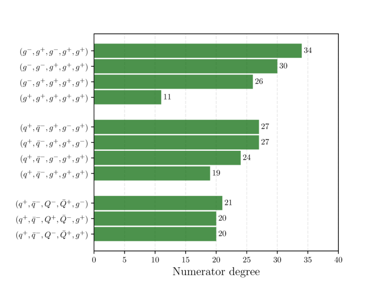
Finally, as an indication for the complexity of the analytic reconstruction we show the numerator degrees for the contribution of all the planar five-parton remainders in figure 8. The figure displays the expected reduction in complexity of the remainders for external fermions compared to gluons.

4.2 Basis of Rational Coefficients
It was noted in Abreu:2018aqd; Chicherin:2018yne; Abreu:2019rpt; Chicherin:2019xeg that the space of independent rational functions appearing in the super Yang-Mills (SYM) and super gravity two-loop five-point amplitudes is much smaller than the space of possible independent pentagon functions. This motivates us to apply the same analysis here, both in order to allow performing minimal reconstruction work and as a way to obtain simpler analytic expressions. These linear dependencies between the rational functions allow us to express the remainder of each amplitude as
| (41) |
where is a vector of rational coefficients and denotes the dimension of the space they span. The index runs over a subspace of the space of all pentagon functions introduced in eq. (17), i.e., . The constant matrix , the rational functions and the index sets and are helicity-amplitude dependent.
The basis of rational functions is not unique and we choose it by taking the linearly independent subset with the lowest total polynomial degree. The associated matrix can be computed numerically in the finite field used for the analytic reconstruction, using as many evaluations as its rank. In order to rationally reconstruct we only require one finite field of cardinality , apart from two cases where we combine information from two finite fields (see more details in section 5).
4.3 Partial Fractions
Having chosen a basis of rational coefficients, we study the in a finite field, obtained with the strategy described in section (4.1). The next step is to lift the finite-field result to the rational numbers, i.e., to rationally reconstruct the result. The correctness of the rational reconstruction can be verified by comparison against a single evaluation on a different finite field. In general, the success of the rational reconstruction is guaranteed if the numerator and denominator of the original rational number satisfy a bound dependent on the finite-field cardinality Wang:1981:PAU:800206.806398; vonManteuffel:2014ixa; Peraro:2016wsq, i.e., rational numbers with numerators and denominators with smaller absolute values are more easily reconstructed from their finite-field images. As such, it is beneficial if we can find a form of the where the rational numbers involved have ‘simple’ numerators and denominators. To this end, we will employ a multivariate partial-fraction decomposition of the , which will also have the side effect of simplifying their analytic form as a whole. Indeed, the partial-fraction decomposition manifests the singularities of the coefficients, which are controlled by physical properties such as the factorization of the amplitude in specific limits.
We will employ the partial-fraction decomposition introduced by Leĭnartas leinartas1978factorization; raichev2012leinartas. This decomposition has recently been used for bringing differential equations into canonical form Meyer:2016slj, as well as for the analytic reduction of loop integrands Zhang:2012ce; Mastrolia:2012an. A Leĭnartas decomposition of our basis functions is given by
| (42) |
That is, the are written as a linear combination of rational functions which we label by the exponents of the denominators. The set of all for a given is denoted by (we combine the exponents for the even and odd coefficients). The are the numerators associated with the rational function labelled by , which are polynomials in the variables. We construct the Leĭnartas decomposition (42) coefficient-by-coefficient, such that the exponents in are non-vanishing only for the letters appearing in the starting denominator , see eq. (37), which we recall are polynomials in the . The particular algorithm which we employ to uniquely specify the Leĭnartas decomposition is related to the techniques of Smirnov:2005ky.
A Leĭnartas decomposition (42) is characterized by exponents of the denominator factors. All denominators in a Leĭnartas decomposition are ‘algebraically independent’, in that there exists no non-zero polynomial , such that it vanishes upon inserting the denominator factors,
| (43) |
where denotes the set of letters in , see eq. (21). Let us make a few comments about such a decomposition. First, individual terms in eq. (42) may have factors raised to higher degree than when expressed over a common denominator as in eq. (37). Second, no term can have more denominator factors than the number of variables as these factors would necessarily be algebraically dependent. Also, we note that the Leĭnartas decomposition is different to an iterated univariate partial-fraction decomposition in that it maintains the original denominator structures of the input function, i.e., in our case, of eq. (37). Finally, in ref. raichev2012leinartas it is noted that such a decomposition is in general not unique, due to how the algebraic dependence relations (43) are resolved. Let us illustrate this point by considering
| (44) |
which clearly vanishes upon using the definitions of the letters, and . The dependence relation implies a relation between multiple terms with different denominator factors,
| (45) |
which can be used to remove either of the three denominator factors on the right-hand side. This arbitrariness in the implementation of the Leĭnartas decomposition will in general lead to expressions that are not as compact as possible if inconsistent choices are made across different terms being decomposed. In the following we describe an approach that produces a unique Leĭnartas decomposition by providing a global prescription to expand algebraic dependencies of the denominators of a given coefficient .
Our approach makes use of multivariate polynomial division and Gröbner basis techniques. In summary, we reinterpret a rational function in a polynomial way in order to employ division by a Gröbner basis to find a canonical form of a polynomial which is subject to a series of constraints. The set of constraints among the variables form a generating set of an ideal and if one divides a polynomial in these variables by a Gröbner basis of the ideal, the remainder is unique and ‘minimal’ with respect to the relations. In the rest of this section we describe these steps in more detail. We refer the reader to ref. cox2013ideals for a pedagogical discussion of all the required concepts in polynomial-division algorithms.
Our starting point is a rational function of the form (37), and we introduce an auxiliary variable for each denominator factor for , where we recall denotes the set of labels of letters appearing in the denominator of . More precisely we introduce variables to which we associate the constraint polynomial ,
| (46) |
Setting all (i.e., working in the equivalence class of the ideal generated by ) imposes the constraint that multiplication by is equivalent to division by . As such, subject to this constraint we can express eq. (37) in a polynomial fashion as
| (47) |
where the notation ’’ emphasises that the relation holds modulo the ideal . In order to uniquely implement the constraints , we first divide the right-hand side of eq. (47) by a Gröbner basis of the constraint polynomials .33 3 It is important to note that Gröbner basis division works over any field. Hence, the algorithm can be be applied before or after rational reconstruction. After the division, the original polynomial is rewritten as a linear combination of the and a unique remainder, which is a polynomial in the and the . We then impose , leaving this remainder as the result of the partial-fraction decomposition. Finally, we replace the by and recover an expression of the form of eq. (42). We note that the Gröbner basis of the ideal depends on a monomial ordering of the variables and , which in turn affects the final expression. Effectively, by choosing different orderings one can specify which of the denominator factors one prefers in the final expression. Once this choice has been made, the result of the procedure is unique.
Let us now comment on why this simple polynomial division technique achieves a minimal Leĭnartas decomposition. First, it is important to recall that the remainder of the division by a Gröbner basis is minimal in the sense that it cannot be written in terms of a member of the ideal and a new remainder without that remainder having higher polynomial degree. That is, subject to the choice of monomial ordering, the remainder has the lowest possible polynomial degree. With this in mind, it is clear why the division by the constraint polynomials (46) will maximally cancel numerator and denominator: since the second term of the constraint polynomial is , which is the term with the lowest possible degree (in any monomial orderings), all possible cancellations between numerator and denominator will occur, as that ensures they will result in the lowest polynomial degree for the remainder.
Another important question is how this division results in a set of denominator structures with no algebraic dependencies, see eq. (43), and how the relations are guaranteed to be resolved in a consistent way, see the discussion around eq. (45). The fact that algebraic dependencies are implemented follows from a key property of division by a Gröbner basis, which is that it will also apply non-trivial relations implied by the original set of relations. As already argued in raichev2012leinartas, algebraic dependencies induce such non-trivial relations. Indeed, if the set of denominator factors of a given term
| (48) |
are algebraically dependent, then by definition there exists a non-zero polynomial such that , which is trivially a member of the ideal of constraints. We associate the same monomial ordering to the variables as we do to the and write the polynomial in the form
| (49) |
That is, we distinguish the term of lowest monomial degree (we refer to the notation introduced in eq. (22)). Let us now multiply the in eq. (48) by this polynomial and . We get
| (50) | ||||
where we introduced the function which yields a vector with the negative entries removed. This shows that relations such as that of eq. (45) are now also in the ideal, and we do not have to construct them explicitly. Furthermore, given that by construction , we have
| (51) |
That is, for each term in the sum over , the -dependent part of the monomial is always of lower degree than the original denominator structure . For any monomial ordering where the are sorted before the , the term is thus leading and will therefore be reduced by the polynomial division algorithm, which produces remainders of lower degree. In summary, the algebraic dependence relations are accounted for in the constraint ideal, and will be removed by Gröbner basis division. If, for instance, one chooses a lexicographic order (with the ’s sorted before the variables), this will decrease the power of the for the lowest , at the price of potentially increasing the power of for higher . This argument can be applied recursively until all algebraic dependencies have been resolved. Because the resolution of the dependencies is based on the polynomial ordering and implemented by the Gröbner basis division, it will be consistently implemented across all denominator factors of a given and give a unique Leĭnartas decomposition.
We close by noting that this procedure is both simple to implement as well as very efficient, easily handling the complex rational functions present in the problem. Furthermore, an important consequence of this decomposition is that the rational numbers in the expression are more likely to be small. As discussed at the beginning of this section, this makes the result in a single finite field of cardinality sufficient to determine them.
5 Results
In this section we take a closer look at the analytic results we derived for a basis set of two-loop five-parton amplitudes. We list the checks we have performed and describe the format of the ancillary files which are used to distribute the results. We also comment on the structure of the remainders.
For each five-parton process we choose a basis set of helicity amplitudes, such that all other choices of helicities and color structures from eqs. 3, 4 and 5 can be obtained by a combination of parity transformation, charge conjugation, and permutations of external momenta. Since we reconstruct two-loop remainders, in order to assemble two-loop amplitudes we also need expressions for the one-loop amplitudes through order , see eq. (10). Hence, we have computed analytic expressions for all the corresponding leading-color one-loop amplitudes to all orders in in the HV scheme (extending corresponding results of Bern:1993mq; Kunszt:1994nq; Bern:1994fz) and checked that they reproduce the numerical one-loop results presented in Abreu:2018jgq up to . The calculation of these amplitudes was also performed by analytically reconstructing the expressions from numerical data.
In order to validate the expressions of the finite two-loop remainders, we have performed a number of checks. First, to check the correctness of the reconstruction procedure, we have compared our analytic results to an independent numerical evaluation of the amplitude on rational phase-space points and found agreement. Second, we have used the analytic results for one-loop amplitudes and two-loop remainders to reproduce all available numerical targets Badger:2013gxa; Badger:2017jhb; Gehrmann:2015bfy; Abreu:2017hqn; Badger:2018gip; Abreu:2018jgq; Dunbar:2016aux. Finally, the analytic results presented here for five-gluon amplitudes at agree with the previously computed expressions Gehrmann:2015bfy; Dunbar:2016aux; Badger:2018enw; Abreu:2018zmy.
We present our results in the form of ancillary files which can be downloaded from the source files of this work on the arXiv server. We include the following files, in Mathematica-readable format:
- •
Analytic expressions for the basis set of one-loop five-parton amplitudes expressed in terms of one-loop master integrals, valid to all orders in ;
- •
Expressions for all one-loop master integrals written in terms of pentagon functions through order ;
- •
The basis set of two-loop five-parton finite remainders, which are the main result of this work. For each remainder and at each power of , we give a list of independent coefficient functions , a matrix and a list of pentagon functions , consistent with the decomposition of eq. (41);
- •
Scripts that assemble two-loop amplitudes from the remainders. In particular, the Mathematica script TwoLoopAmplitudesNumerical.m uses the analytic expressions to reproduce the numeric values of refs. Abreu:2018jgq; Badger:2018gip, as detailed in the included README.md file.
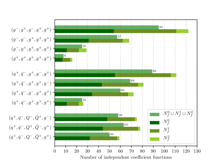
Our expressions can be easily adapted to perform numerical integration over phase space. Indeed, they are very compact (with a compressed size of 1.6 Mb), and ready for automated algorithms for optimized evaluation like those included in FORM Kuipers:2012rf; Ruijl:2014spa. It is interesting to note that whilst there are around 400 independent pentagon functions, for all amplitudes the number of independent rational structures is much lower. A further simplification of the coefficients can be obtained by combining different powers of in a decomposition similar to that of eq. (41). Indeed, in figure 9 we observe an overlap of the spaces of independent coefficients functions between distinct contributions for a given helicity assignment (these are expected from the cancellations present in supersymmetric amplitudes). For the most complicated amplitude, , the dimension of the combined set of coefficient functions is only 95. We have not presented the amplitudes in this way in the expressions we provide in order to give easier access to the different powers of . While our expressions are specialized to the Euclidean phase-space region, our coefficients can be used to extract the required information to cover all regions of phase space with minimal work. We leave this to a future publication, where we will explore the numerical evaluation of the amplitudes in more detail.
We end this section by summarizing the computational resources used to obtain our results. The evaluation of the multivariate polynomials in eq. (37), which is performed in a single finite field for all processes, is the most computationally intense. Every other step of the computation, including the extraction of denominator factors, the construction of the matrix , 44 4 We note that, for all processes considered, the matrix was computed with only the information contained in the , except for the remainder of the processes and where, in order to rationally reconstruct its entries, the numerical computation of the remainder over 100 extra phase-space points in a second finite field was required. performing the partial fractioning of the expressions and rationally reconstructing the numerical coefficients obtained in the previous step, can be performed quickly on a modern laptop computer. The most demanding remainder reconstruction was that of the contribution to the process. In total, 94,696 phase-space points (coming in parity conjugate pairs, as discussed in section 4.1) were necessary for its reconstruction. On average (considering all contributions to the reconstruction procedure) the evaluation time per phase-space point amounts to 4.5 minutes.55 5 This timing information is measured on an Intel Xeon E5-2670v3 CPU while running the maximum amount of threads it allows. The total computational resources required to evaluate all our results are relatively modest, and can easily be obtained on a midsize computer cluster.
6 Conclusion
We have presented the leading-color five-parton two-loop scattering amplitudes in analytic form for the first time. These are provided in a set of ancillary files, where we give compact analytic expressions for five-gluon amplitudes as well as amplitudes with two and four external quarks, including in all cases the contributions of closed light-quark loops. These results have been obtained employing a functional-reconstruction approach Peraro:2016wsq to promote numerical unitarity Ita:2015tya; Abreu:2017xsl; Abreu:2017idw finite-field evaluations of the amplitude to analytical expressions.
This approach has recently been applied for the planar five-gluon two-loop amplitudes in ref. Abreu:2018zmy and here we develop it further in two main directions. First, we have improved the handling of fermions in the numerical approach. We use dimensional reduction to analytically obtain part of the dependence on the dimensional-regularization parameter by introducing scalar particles. This leads to significant efficiency improvements as compared to a numerical dimensional-reconstruction approach Giele:2008ve; Ellis:2008ir; Boughezal:2011br as applied earlier in refs. Abreu:2017xsl; Abreu:2017hqn; Abreu:2018jgq. Enhancing the dimensional reconstruction by dimensional reduction is not a new idea and has been applied to gluon amplitudes in the original work Giele:2008ve. Here we apply this improvement Anger:2018ove starting from the five-point amplitudes including external fermions Abreu:2018jgq. Second, we have improved the analytic-reconstruction algorithm from numerical samples. We reconstruct directly in terms of Mandelstam variables as opposed to momentum-twistor variables, which requires considerably fewer evaluations. Furthermore, we simplify the reconstruction procedure by focusing on a linearly independent set of rational functions. Moreover, we have developed a multivariate partial-fraction algorithm in order to perform rational reconstruction with input from only a single finite field of cardinality . As a by-product of these techniques, we find compact analytic forms and an interestingly small set of independent functions. With these methods, a sample with a size comparable to that required for numerical Monte-Carlo integration can be used to produce analytic expressions.
The computational method we present is robust and efficient. Here, we computed compact analytic expressions for QCD amplitudes depending on five kinematic scales, which had long been a bottleneck. We expect that important scattering amplitudes in the Standard Model depending on a higher number of scales are within the reach of our approach. With the recent progress in non-planar master integral computations Abreu:2018aqd; Chicherin:2018old, it would also be interesting to explore the amplitudes beyond the leading-color approximation.
The five-parton amplitudes are an important ingredient for obtaining precision phenomenology for the three-jet production process at next-to-next-to-leading order QCD at the LHC in the coming years. In particular, a complete set of compact analytic expressions, such as the ones presented here, will be important for an efficient and numerically stable evaluation of the amplitudes. On a shorter time scale, we believe that our results will be valuable for exploring the analytic properties of scattering amplitudes in QCD.
Acknowledgments
We thank L. J. Dixon, D. A. Kosower and M. Zeng for many useful discussions. We thank C. Duhr for the use of his Mathematica package PolyLogTools. The work of S.A. is supported by the Fonds de la Recherche Scientifique–FNRS, Belgium. The work of J.D., F.F.C. and V.S. is supported by the Alexander von Humboldt Foundation, in the framework of the Sofja Kovalevskaja Award 2014, endowed by the German Federal Ministry of Education and Research. The work of B.P. is supported by the French Agence Nationale pour la Recherche, under grant ANR–17–CE31–0001–01. The authors acknowledge support by the state of Baden-Württemberg through bwHPC and the German Research Foundation (DFG) through grant no INST 39/963-1 FUGG.
Appendix A Infrared Structure of Two-Loop Five-Parton Amplitudes
In this appendix we give more details on our definition of the remainders we compute in this paper. In section 2.2 we stated that divergences of renormalized two-loop amplitudes obey a universal structure,
| (52) | ||||
The renormalized amplitudes can be written in terms of the bare amplitudes as
| (53) | ||||
with
| (54) |
For amplitudes in the leading-color approximation the operators and are diagonal in color space. The operator is given by
| (55) |
with and the indices defined cyclically. The index denotes a type of particle with momentum , i.e., . The symbols are symmetric under the exchange of indices, , and given by:
| (56) | ||||
The operator is
| (57) |
where
| (58) |
and is a diagonal operator at leading color that depends on the number of external quarks and gluons in the process,
| (59) | ||||
with
| (60) | ||||
The two-loop bare amplitude can be obtained from the remainder defined in eq. (11) using
| (61) | ||||
Appendix B Dimensionally Reduced Feynman Rules
In the table 1 we list the color-ordered Feynman rules for vertices involving the scalar particles introduced in section 3. The -dimensional part of these rules can be fully contracted in each Feynman diagram yielding kinematic-independent factors.
Appendix C Rational Phase-Space Parametrization
We give a twistor parametrization Hodges:2009hk used to rationalize the external on-shell momenta with . This parametrization yields a momentum point with the kinematic invariants from the input variables and as given in the main text in eq. (32).
To each external momentum , we associate the spinors and , from which we can compute the associated momenta through
| (62) |
The spinors are then parametrized through the momentum-twistor matrix,
| (63) |
Conjugate spinors can then be obtained through
| (64) |
where is the usual spinor-bracket computed by taking the determinant of the associated sub-matrix of (63). The Mandelstam invariants and required in the main text are given in terms of spinors by,
| (65) |
using . For further details, see e.g. section 2 of ref. Bourjaily:2010wh.
References
- (1) S. Badger, H. Frellesvig and Y. Zhang, A Two-Loop Five-Gluon Helicity Amplitude in QCD, JHEP 12 (2013) 045 [1310.1051].
- (2) T. Gehrmann, J. M. Henn and N. A. Lo Presti, Analytic form of the two-loop planar five-gluon all-plus-helicity amplitude in QCD, Phys. Rev. Lett. 116 (2016) 062001 [1511.05409].
- (3) D. C. Dunbar and W. B. Perkins, Two-loop five-point all plus helicity Yang-Mills amplitude, Phys. Rev. D93 (2016) 085029 [1603.07514].
- (4) D. C. Dunbar, G. R. Jehu and W. B. Perkins, Two-loop six gluon all plus helicity amplitude, Phys. Rev. Lett. 117 (2016) 061602 [1605.06351].
- (5) D. C. Dunbar, J. H. Godwin, G. R. Jehu and W. B. Perkins, Analytic all-plus-helicity gluon amplitudes in QCD, Phys. Rev. D96 (2017) 116013 [1710.10071].
- (6) S. Badger, C. Brønnum-Hansen, H. B. Hartanto and T. Peraro, First look at two-loop five-gluon scattering in QCD, Phys. Rev. Lett. 120 (2018) 092001 [1712.02229].
- (7) S. Abreu, F. Febres Cordero, H. Ita, B. Page and M. Zeng, Planar Two-Loop Five-Gluon Amplitudes from Numerical Unitarity, Phys. Rev. D97 (2018) 116014 [1712.03946].
- (8) S. Badger, C. Brønnum-Hansen, T. Gehrmann, H. B. Hartanto, J. Henn, N. A. Lo Presti et al., Applications of integrand reduction to two-loop five-point scattering amplitudes in QCD, in 14th DESY Workshop on Elementary Particle Physics: Loops and Legs in Quantum Field Theory 2018 (LL2018) St Goar, Germany, April 29-May 4, 2018, 2018, 1807.09709.
- (9) S. Abreu, F. Febres Cordero, H. Ita, B. Page and V. Sotnikov, Planar Two-Loop Five-Parton Amplitudes from Numerical Unitarity, JHEP 11 (2018) 116 [1809.09067].
- (10) T. Peraro, Scattering amplitudes over finite fields and multivariate functional reconstruction, JHEP 12 (2016) 030 [1608.01902].
- (11) S. Badger, C. Brønnum-Hansen, H. B. Hartanto and T. Peraro, Analytic helicity amplitudes for two-loop five-gluon scattering: the single-minus case, JHEP 01 (2019) 186 [1811.11699].
- (12) S. Abreu, J. Dormans, F. Febres Cordero, H. Ita and B. Page, Analytic Form of Planar Two-Loop Five-Gluon Scattering Amplitudes in QCD, Phys. Rev. Lett. 122 (2019) 082002 [1812.04586].
- (13) C. G. Papadopoulos, D. Tommasini and C. Wever, The Pentabox Master Integrals with the Simplified Differential Equations approach, JHEP 04 (2016) 078 [1511.09404].
- (14) T. Gehrmann, J. M. Henn and N. A. Lo Presti, Pentagon functions for massless planar scattering amplitudes, JHEP 10 (2018) 103 [1807.09812].
- (15) S. Badger, G. Mogull, A. Ochirov and D. O’Connell, A Complete Two-Loop, Five-Gluon Helicity Amplitude in Yang-Mills Theory, JHEP 10 (2015) 064 [1507.08797].
- (16) S. Abreu, L. J. Dixon, E. Herrmann, B. Page and M. Zeng, The two-loop five-point amplitude in super-Yang-Mills theory, Phys. Rev. Lett. 122 (2019) 121603 [1812.08941].
- (17) D. Chicherin, T. Gehrmann, J. M. Henn, P. Wasser, Y. Zhang and S. Zoia, All master integrals for three-jet production at NNLO, 1812.11160.
- (18) R. H. Boels, Q. Jin and H. Luo, Efficient integrand reduction for particles with spin, 1802.06761.
- (19) H. A. Chawdhry, M. A. Lim and A. Mitov, Two-loop five-point massless QCD amplitudes within the IBP approach, 1805.09182.
- (20) G. Ossola, C. G. Papadopoulos and R. Pittau, Reducing full one-loop amplitudes to scalar integrals at the integrand level, Nucl. Phys. B763 (2007) 147 [hep-ph/0609007].
- (21) R. K. Ellis, W. T. Giele and Z. Kunszt, A Numerical Unitarity Formalism for Evaluating One-Loop Amplitudes, JHEP 03 (2008) 003 [0708.2398].
- (22) W. T. Giele, Z. Kunszt and K. Melnikov, Full one-loop amplitudes from tree amplitudes, JHEP 04 (2008) 049 [0801.2237].
- (23) C. F. Berger, Z. Bern, L. J. Dixon, F. Febres Cordero, D. Forde, H. Ita et al., An Automated Implementation of On-Shell Methods for One-Loop Amplitudes, Phys. Rev. D78 (2008) 036003 [0803.4180].
- (24) Z. Bern, L. J. Dixon, D. C. Dunbar and D. A. Kosower, One-loop n-point gauge theory amplitudes, unitarity and collinear limits, Nucl. Phys. B425 (1994) 217 [hep-ph/9403226].
- (25) Z. Bern, L. J. Dixon, D. C. Dunbar and D. A. Kosower, Fusing gauge theory tree amplitudes into loop amplitudes, Nucl. Phys. B435 (1995) 59 [hep-ph/9409265].
- (26) Z. Bern, L. J. Dixon and D. A. Kosower, One-loop amplitudes for to four partons, Nucl. Phys. B513 (1998) 3 [hep-ph/9708239].
- (27) R. Britto, F. Cachazo and B. Feng, Generalized unitarity and one-loop amplitudes in N=4 super-Yang-Mills, Nucl. Phys. B725 (2005) 275 [hep-th/0412103].
- (28) H. Ita, Two-loop Integrand Decomposition into Master Integrals and Surface Terms, Phys. Rev. D94 (2016) 116015 [1510.05626].
- (29) S. Abreu, F. Febres Cordero, H. Ita, M. Jaquier and B. Page, Subleading Poles in the Numerical Unitarity Method at Two Loops, Phys. Rev. D95 (2017) 096011 [1703.05255].
- (30) S. Abreu, F. Febres Cordero, H. Ita, M. Jaquier, B. Page and M. Zeng, Two-Loop Four-Gluon Amplitudes from Numerical Unitarity, Phys. Rev. Lett. 119 (2017) 142001 [1703.05273].
- (31) A. von Manteuffel and R. M. Schabinger, A novel approach to integration by parts reduction, Phys. Lett. B744 (2015) 101 [1406.4513].
- (32) F. R. Anger and V. Sotnikov, On the Dimensional Regularization of QCD Helicity Amplitudes With Quarks, 1803.11127.
- (33) R. K. Ellis, W. T. Giele, Z. Kunszt and K. Melnikov, Masses, fermions and generalized -dimensional unitarity, Nucl. Phys. B822 (2009) 270 [0806.3467].
- (34) R. Boughezal, K. Melnikov and F. Petriello, The four-dimensional helicity scheme and dimensional reconstruction, Phys. Rev. D84 (2011) 034044 [1106.5520].
- (35) A. Hodges, Eliminating spurious poles from gauge-theoretic amplitudes, JHEP 05 (2013) 135 [0905.1473].
- (36) E. W. N. Glover, Two loop QCD helicity amplitudes for massless quark quark scattering, JHEP 04 (2004) 021 [hep-ph/0401119].
- (37) A. De Freitas and Z. Bern, Two-loop helicity amplitudes for quark-quark scattering in QCD and gluino-gluino scattering in supersymmetric Yang-Mills theory, JHEP 09 (2004) 039 [hep-ph/0409007].
- (38) S. Catani, The Singular behavior of QCD amplitudes at two loop order, Phys. Lett. B427 (1998) 161 [hep-ph/9802439].
- (39) G. F. Sterman and M. E. Tejeda-Yeomans, Multi-loop amplitudes and resummation, Phys. Lett. B552 (2003) 48 [hep-ph/0210130].
- (40) T. Becher and M. Neubert, Infrared singularities of scattering amplitudes in perturbative QCD, Phys. Rev. Lett. 102 (2009) 162001 [0901.0722].
- (41) E. Gardi and L. Magnea, Factorization constraints for soft anomalous dimensions in QCD scattering amplitudes, JHEP 03 (2009) 079 [0901.1091].
- (42) R. Baumeister, D. Mediger, J. Pečovnik and S. Weinzierl, On the vanishing of certain cuts or residues of loop integrals with higher powers of the propagators, 1903.02286.
- (43) J. Vollinga and S. Weinzierl, Numerical evaluation of multiple polylogarithms, Comput. Phys. Commun. 167 (2005) 177 [hep-ph/0410259].
- (44) A. B. Goncharov, M. Spradlin, C. Vergu and A. Volovich, Classical Polylogarithms for Amplitudes and Wilson Loops, Phys. Rev. Lett. 105 (2010) 151605 [1006.5703].
- (45) C. Duhr, H. Gangl and J. R. Rhodes, From polygons and symbols to polylogarithmic functions, JHEP 10 (2012) 075 [1110.0458].
- (46) C. Duhr, Hopf algebras, coproducts and symbols: an application to Higgs boson amplitudes, JHEP 08 (2012) 043 [1203.0454].
- (47) D. Cox, J. Little and D. O’Shea, Ideals, Varieties, and Algorithms, Undergraduate Texts in Mathematics. Springer, Cham, 2015, https://doi.org/10.1007/978-3-319-16721-3.
- (48) P. Nogueira, Automatic Feynman graph generation, J. Comput. Phys. 105 (1993) 279.
- (49) A. Ochirov and B. Page, Full Colour for Loop Amplitudes in Yang-Mills Theory, JHEP 02 (2017) 100 [1612.04366].
- (50) A. Ochirov and B. Page, Multi-quark colour decompositions from unitarity, in preparation (2019) .
- (51) W. Decker, G.-M. Greuel, G. Pfister and H. Schönemann, “Singular 4-1-0 — A computer algebra system for polynomial computations.” http://www.singular.uni-kl.de, 2016.
- (52) T. Gautier, J.-L. Roch and G. Villard, “Givaro.” https://casys.gricad-pages.univ-grenoble-alpes.fr/givaro/, 2017.
- (53) P. Barrett, Implementing the Rivest Shamir and Adleman Public Key Encryption Algorithm on a Standard Digital Signal Processor. Springer, Berlin, Heidelberg, 1987, 10.1007/3-540-47721-7_24.
- (54) J. van der Hoeven, G. Lecerf and G. Quintin, Modular SIMD arithmetic in mathemagix, CoRR abs/1407.3383 (2014) [1407.3383].
- (55) F. A. Berends and W. T. Giele, Recursive Calculations for Processes with n Gluons, Nucl. Phys. B306 (1988) 759.
- (56) F. R. Anger, F. Febres Cordero, H. Ita and V. Sotnikov, NLO QCD predictions for production in association with up to three light jets at the LHC, Phys. Rev. D97 (2018) 036018 [1712.05721].
- (57) J. C. Collins, Renormalization, vol. 26 of Cambridge Monographs on Mathematical Physics. Cambridge University Press, Cambridge, 1986, 10.1017/CBO9780511622656.
- (58) M. Kreuzer, “Lecture notes: Supersymetry.” http://hep.itp.tuwien.ac.at/˜kreuzer/inc/susy.pdf, 2010.
- (59) Z. Bern, A. De Freitas, L. J. Dixon and H. L. Wong, Supersymmetric regularization, two loop QCD amplitudes and coupling shifts, Phys. Rev. D66 (2002) 085002 [hep-ph/0202271].
- (60) D. Chicherin, J. M. Henn, P. Wasser, T. Gehrmann, Y. Zhang and S. Zoia, Analytic result for a two-loop five-particle amplitude, Phys. Rev. Lett. 122 (2019) 121602 [1812.11057].
- (61) S. Abreu, L. J. Dixon, E. Herrmann, B. Page and M. Zeng, The two-loop five-point amplitude in = 8 supergravity, JHEP 03 (2019) 123 [1901.08563].
- (62) D. Chicherin, T. Gehrmann, J. M. Henn, P. Wasser, Y. Zhang and S. Zoia, The two-loop five-particle amplitude in = 8 supergravity, JHEP 03 (2019) 115 [1901.05932].
- (63) P. S. Wang, A p-adic algorithm for univariate partial fractions, in Proceedings of the Fourth ACM Symposium on Symbolic and Algebraic Computation, SYMSAC ’81, (New York, NY, USA), pp. 212–217, ACM, 1981, DOI.
- (64) E. K. Leinartas, Factorization of rational functions of several variables into partial fractions, Izvestiya Vysshikh Uchebnykh Zavedenii. Matematika (1978) 47.
- (65) A. Raichev, Leinartas’s partial fraction decomposition, 1206.4740.
- (66) C. Meyer, Transforming differential equations of multi-loop Feynman integrals into canonical form, JHEP 04 (2017) 006 [1611.01087].
- (67) Y. Zhang, Integrand-Level Reduction of Loop Amplitudes by Computational Algebraic Geometry Methods, JHEP 09 (2012) 042 [1205.5707].
- (68) P. Mastrolia, E. Mirabella, G. Ossola and T. Peraro, Scattering Amplitudes from Multivariate Polynomial Division, Phys. Lett. B718 (2012) 173 [1205.7087].
- (69) A. V. Smirnov and V. A. Smirnov, Applying Grobner bases to solve reduction problems for Feynman integrals, JHEP 01 (2006) 001 [hep-lat/0509187].
- (70) Z. Bern, L. J. Dixon and D. A. Kosower, One loop corrections to five gluon amplitudes, Phys. Rev. Lett. 70 (1993) 2677 [hep-ph/9302280].
- (71) Z. Kunszt, A. Signer and Z. Trocsanyi, One loop radiative corrections to the helicity amplitudes of QCD processes involving four quarks and one gluon, Phys. Lett. B336 (1994) 529 [hep-ph/9405386].
- (72) Z. Bern, L. J. Dixon and D. A. Kosower, One loop corrections to two quark three gluon amplitudes, Nucl. Phys. B437 (1995) 259 [hep-ph/9409393].
- (73) J. Kuipers, T. Ueda, J. A. M. Vermaseren and J. Vollinga, FORM version 4.0, Comput. Phys. Commun. 184 (2013) 1453 [1203.6543].
- (74) B. Ruijl, A. Plaat, J. Vermaseren and J. van den Herik, Why Local Search Excels in Expression Simplification, 1409.5223.
- (75) J. L. Bourjaily, Efficient Tree-Amplitudes in N=4: Automatic BCFW Recursion in Mathematica, 1011.2447.