Functional Liftings of Vectorial Variational Problems with Laplacian Regularization

Let $\Omega\subset\mathbb{R}^{d}$ and $\Gamma\subset\mathbb{R}^{s}$ both be bounded sets. In the following, we consider the variational problem of minimizing the functional

that acts on vector-valued functions $u\in C^{2}(\Omega;\Gamma)$. Convexity of the integrand $f\colon\Omega\times\Gamma\times\mathbb{R}^{s}\to\mathbb{R}$ is only assumed in the last entry, so that $u\mapsto F(u)$ is generally non-convex. The Laplacian $\Delta u$ is understood component-wise and reduces to $u^{\prime\prime}$ if the domain $\Omega$ is one-dimensional.

Variational problems of this form occur in a wide variety of image processing tasks, including image reconstruction, restoration, and interpolation. Commonly, the integrand is split into data term and regularizer:

As an example, in image registration (sometimes referred to as large-displacement optical flow), the data term $\rho(x,z)=d(R(x),T(x+z))$ encodes the pointwise distance of a reference image $R\colon\mathbb{R}^{d}\to\mathbb{R}^{k}$ to a deformed template image $T\colon\mathbb{R}^{d}\to\mathbb{R}^{k}$ according to a given distance measure $d(\cdot,\cdot)$, such as the squared Euclidean distance $d(a,b)=\frac{1}{2}\|a-b\|_{2}^{2}$. While often a suitable convex regularizer $\eta$ can be found, the highly non-convex nature of $\rho$ renders the search for global minimizers of (1) a difficult problem.

Instead of directly minimizing $F$ using gradient descent or other local solvers, we will aim to replace it by a convex functional $\mathcal{F}$ that acts on a higher-dimensional (lifted) function space. If the lifting is chosen in such a way that we can construct global minimizers of $F$ from global minimizers of $\mathcal{F}$, we can find a global solution of the original problem by applying convex solvers to $\mathcal{F}$. While we cannot claim this property for our choice of lifting, we believe that the mathematical motivation and some of the experimental results show that this approach can be a good basis for future work on global solutions of variational models with higher-order regularization.

where $F$ acts on functions $u\colon\Omega\to\Gamma$ with $\Omega\subset\mathbb{R}^{d}$ and scalar range $\Gamma\subset\mathbb{R}$.

The calibration method as introduced in [1] gives a globally sufficient optimality condition for functionals of the form (3) with $\Gamma=\mathbb{R}$. Importantly, $f(x,z,p)$ is not required to be convex in $(x,z)$, but only in $p$. The method states that $u$ minimizes $F$ if there exists a divergence-free vector field $\phi\colon\Omega\times\mathbb{R}\to\mathbb{R}^{d+1}$ (a calibration) in a certain admissible set $X$ of vector fields on $\Omega\times\mathbb{R}$ (see below for details), such that

where $\mathbf{1}_{u}$ is the characteristic function of the subgraph of $u$ in $\Omega\times\mathbb{R}$, $\mathbf{1}_{u}(x,z)=1$ if $u(x)>z$ and $0$ otherwise, and $D\mathbf{1}_{u}$ is its distributional derivative. The duality between subgraphs and certain vector fields is also the subject of the broader theory of Cartesian currents [8].

A convex relaxation of the original minimization problem then can be formulated in a higher-dimensional space by considering the functional [5, 19]

acting on functions $v$ from the convex set

In both formulations, the set of admissible test functions is

where $f^{*}(x,z,p):=\sup_{q}\langle p,q\rangle-f(x,z,q)$ is the convex conjugate of $f$ with respect to the last variable. In fact, the equality

has been argued to hold for $u\in W^{1,1}(\Omega)$ under suitable assumptions on $f$ [19]. A rigorous proof of the case of $u\in BV(\Omega)$ and $f(x,z,p)=f(z,p)$ ($f$ independent of $x$), but not necessarily continuous in $z$, can be found in the recent work [2].

In [17], it is discussed how the choice of discretization influences the results of numerical implementations of this approach. More precisely, motivated by the work [18] from continuous multilabeling techniques, the choice of piecewise linear finite elements on $\Gamma$ was shown to exhibit so-called sublabel-accuracy, which is known to significantly reduce memory requirements.

There are functional lifting approaches for vectorial data with first-order regularization that consider the subgraphs of the components of $u$ [9, 21]. It is not clear how to generalize this approach to nonlinear data $\Gamma\subset\mathcal{M}$, such as a manifold $\mathcal{M}$, where other functional lifting approaches exist at least for the case of total variation regularization [14].

An approach along the lines of [18] for vectorial data with total variation regularization was proposed in [12]. Even though [17] demonstrated how [18] can be interpreted as a discretized version of the calibration-based lifting, the equivalent approach [12] for vectorial data lacks a fully-continuous formulation as well as a generalization to arbitrary integrands that would demonstrate the exact connection to the calibration method.

We implemented the proposed model in Python 3 with NumPy and PyCUDA. The examples were computed on an Intel Core i7 4.00 GHz with 16 GB of memory and an NVIDIA GeForce GTX 1080 Ti with 12 GB of dedicated video memory. The iteration was stopped when the Euclidean norms of the primal and dual residuals [10] fell below $10^{-6}\cdot\sqrt{n}$ where $n$ is the respective number of variables.

In the first experiment (Figure 1), the reference image $R$ was synthesized by numerically rotating the template $T$ by $40$ degrees. The grid plot of the computed deformation as well as the deformed template are visually very close to the rigid ground-truth deformation (a rotation by 40 degrees). Note that the method obtains almost pixel-accurate results although the range $\Gamma$ of the deformation is discretized on a disk around the origin, triangulated using only $25$ vertices, which is far less than the image resolution.

The second experiment (Figure 2) consists of two coronal slices from a DCE-MRI dataset of a human kidney (data courtesy of Jarle Rørvik, Haukeland University Hospital Bergen, Norway; taken from [3]). The deformation computed using our proposed model is able to significantly reduce the misfit in liver and kidney in the left half while accurately fixing the spinal cord at the right edge.

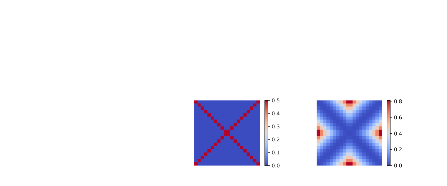
To investigate whether a similar property can hold in our higher-order case, we applied our model with Laplacian regularization $\eta(p)=\frac{1}{2}\|p\|^{2}$ as well as the calibration method approach with total variation regularization to the data term $\rho(x,z)=(|x|-|z|)^{2}$ with one-dimensional domain $\Omega=[-1,1]$ and scalar data $\Gamma=[-1,1]$ using $20$ regularly-spaced discretization points (Figure 3).

The result from the first-order approach is easily interpretable as a composition of two solutions to the original problem, each of which can be obtained by thresholding (40). In contrast, thresholding applied to the result from the second-order approach yields the two hat functions $v_{1}(x)=|x|$ and $v_{2}(x)=-|x|$, neither of which minimizes the original functional. Instead, the solution turns out to be of the form $\mathbf{u}=\frac{1}{2}\delta_{u_{1}}+\frac{1}{2}\delta_{u_{2}}$, where $u_{1}$ and $u_{2}$ are in fact global minimizers of the original problem: namely, the straight lines $u_{1}(x)=x$ and $u_{2}(x)=-x$.

In this work we presented a novel fully-continuous functional lifting approach for non-convex variational problems that involve Laplacian second-order terms and vectorial data, with the aim to ultimately provide sufficient optimality conditions and find global solutions despite the non-convexity. First experiments indicate that the method can produce subpixel-accurate solutions for the non-convex image registration problem. We argued that more involved projection strategies than in the classical calibration approach will be needed for obtaining a good (approximate) solution of the original problem from a solution of the lifted problem. Another interesting direction for future work is the generalization to functionals that involve arbitrary second- or higher-order terms.

References

- [1] Alberti, G., Bouchitté, G., Dal Maso, G.: The calibration method for the mumford-shah functional and free-discontinuity problems. Calculus of Variations and Partial Differential Equations 16(3), 299–333 (Mar 2003)
- [2] Bouchitté, G., Fragalà, I.: A duality theory for non-convex problems in the calculus of variations. Arch Rational Mech Anal 229(1), 361–415 (Jul 2018)
- [3] Brehmer, K., Wacker, B., Modersitzki, J.: A novel similarity measure for image sequences. In: Klein, S., Staring, M., Durrleman, S., Sommer, S. (eds.) Biomedical Image Registration. pp. 47–56. Springer International Publishing, Cham (2018)
- [4] Chambolle, A., Pock, T.: A first-order primal-dual algorithm for convex problems with applications to imaging. J. Math. Imaging Vis. 40(1), 120–145 (2011)
- [5] Chambolle, A.: Convex representation for lower semicontinuous envelopes of functionals in lˆ 1. Journal of Convex Analysis 8(1), 149–170 (2001)
- [6] Chambolle, A., Cremers, D., Pock, T.: A convex approach to minimal partitions. SIAM Journal on Imaging Sciences 5(4), 1113–1158 (2012)
- [7] Fischer, B., Modersitzki, J.: Curvature based image registration. Journal of Mathematical Imaging and Vision 18(1), 81–85 (Jan 2003)
- [8] Giaquinta, M., Modica, G., Souček, J.: Cartesian currents in the calculus of variations I. Cartesian currents., vol. 37. Berlin: Springer (1998)
- [9] Goldluecke, B., Strekalovskiy, E., Cremers, D.: Tight convex relaxations for vector-valued labeling. SIAM Journal on Imaging Sciences 6(3), 1626–1664 (2013)
- [10] Goldstein, T., Esser, E., Baraniuk, R.: Adaptive primal dual optimization for image processing and learning. In: Proc. 6th NIPS Workshop Optim. Mach. Learn. (2013)
- [11] Kleinberg, J., Tardos, E.: Approximation algorithms for classification problems with pairwise relationships: Metric labeling and markov random fields. Journal of the ACM (JACM) 49(5), 616–639 (2002)
- [12] Laude, E., Möllenhoff, T., Moeller, M., Lellmann, J., Cremers, D.: Sublabel-accurate convex relaxation of vectorial multilabel energies. In: European Conference on Computer Vision. pp. 614–627. Springer (2016)
- [13] Lellmann, J., Lenzen, F., Schnörr, C.: Optimality bounds for a variational relaxation of the image partitioning problem. Journal of Mathematical Imaging and Vision 47(3), 239–257 (2013)
- [14] Lellmann, J., Strekalovskiy, E., Koetter, S., Cremers, D.: Total variation regularization for functions with values in a manifold. In: Proceedings of the IEEE International Conference on Computer Vision. pp. 2944–2951 (2013)
- [15] Loewenhauser, B., Lellmann, J.: Functional lifting for variational problems with higher-order regularization. In: Tai, X.C., Bae, E., Lysaker, M. (eds.) Imaging, Vision and Learning Based on Optimization and PDEs. pp. 101–120. Springer International Publishing, Cham (2018)
- [16] Mora, M.G.: The calibration method for free-discontinuity problems on vector-valued maps. Journal of Convex Analysis 9(1), 1–29 (2002)
- [17] Möllenhoff, T., Cremers, D.: Sublabel-accurate discretization of nonconvex free-discontinuity problems. In: Proceedings of the IEEE International Conference on Computer Vision (ICCV) (Oct 2017)
- [18] Möllenhoff, T., Laude, E., Moeller, M., Lellmann, J., Cremers, D.: Sublabel-accurate relaxation of nonconvex energies. In: Proceedings of the IEEE Conference on Computer Vision and Pattern Recognition. pp. 3948–3956 (2016)
- [19] Pock, T., Cremers, D., Bischof, H., Chambolle, A.: Global solutions of variational models with convex regularization. SIAM J. Imaging Sci. 3(4), 1122–1145 (2010)
- [20] Strekalovskiy, E., Chambolle, A., Cremers, D.: A convex representation for the vectorial mumford-shah functional. In: IEEE Conference on Computer Vision and Pattern Recognition (CVPR). pp. 1712–1719. IEEE (2012)
- [21] Strekalovskiy, E., Chambolle, A., Cremers, D.: Convex relaxation of vectorial problems with coupled regularization. SIAM J. Imaging Sci. 7(1), 294–336 (2014)