Stratified Random Sampling for Dependent Inputs
Abstract
A new approach of obtaining stratified random samples from statistically dependent random variables is described. The proposed method can be used to obtain samples from the input space of a computer forward model in estimating expectations of functions of the corresponding output variables. The advantage of the proposed method over the existing methods is that it preserves the exact form of the joint distribution on the input variables. The asymptotic distribution of the new estimator is derived. Asymptotically, the variance of the estimator using the proposed method is less than that obtained using the simple random sampling, with the degree of variance reduction depending on the degree of additivity in the function being integrated. This technique is applied to a practical example related to the performance of the river flood inundation model.
Keywords: Stratified sampling; Latin hypercube sampling; Variance reduction; Sampling with dependent random variables; Monte Carlo simulation.
1 Introduction
Mathematical models are widely used by engineers and scientists to describe physical, economic, and social processes. Often these models are complex in nature and are described by a system of ordinary or partial differential equations, which cannot be solved analytically. Given the values of the input parameters of the processes, complex computer codes are widely used to solve such systems numerically, providing the corresponding outputs. These computer models, also known as forward models, are used for prediction, uncertainty analysis, sensitivity analysis, and model calibration. For such analysis, the computer code is evaluated multiple times to estimate some function of the outputs. However, complex computer codes are often too expensive to be directly used to perform such studies. Design of computer experiment plays an important role in such situations, where the goal is to choose the input configuration in an optimal way such that the uncertainty and sensitivity analysis can be done with a few number of simulation runs. Moreover, to avoid the computation challenge, it is often useful to replace the computer model either by a simpler mathematical approximation called as surrogate or meta model (Volkova et al., 2008, Simpson et al., 2001), or by a statistical approximation, called emulator (Oakley and O’hagan, 2002, O’Hagan, 2006, Conti et al., 2009). Such surrogate models or emulators are also widely used for the model calibration (Kennedy and O’Hagan, 2001), which is the inverse problem of inferring about the model input parameters given the outputs. The surrogate or the emulator model is built based on set of training simulations of the original computer model. The full optimal exploration of the variation domain of the input variables is therefore very important in order to avoid non-informative simulation points (Fang et al., 2006, Sacks et al., 1989).
In most situations, the simple random sampling (SRS) needs very large number of samples to achieve a fixed level of efficiency in estimating some functions of the outputs of such complex models. The required sample size increases rapidly with an increase in dimension of the input space. On the other hand, the Latin hypercube sampling (LHS) introduced by McKay et al., 1979 needs smaller sample sizes than the SRS to achieve the same level of efficiency. Compared to the SRS, which only ensures independence between samples, the LHS also ensures the full coverage of the range of the input variables through stratification over the marginal probability distributions of the inputs. Thus, the LHS method is more efficient and robust if the components of the inputs are independently distributed. In case of dependent inputs Iman and Conover, 1980 has proposed an approximate version of the LHS based on the rank correlation. Stein, 1987 further improved this procedure such that each sample vector has approximately the correct joint distribution when the sample size is large. However, it is noticed that in many scenarios, the rank-based method results in a large bias and small efficiency in the estimators, particularly for small sample sizes. Moreover, the joint distribution of the inputs are also not completely preserved in these sampling schemes even for moderately large sample sizes. Therefore, these rank-based techniques are not very useful for many real applications where one is restricted to a small sample size due to the computational burden of the expensive forward simulator. To overcome this situation, we propose a novel sampling scheme for dependent inputs that precisely gives a random sample from the target joint distribution while keeping the mean squared error of the estimator smaller than the existing methods. In the traditional LHS, where the components of inputs are independent, the stratification of the marginal distributions leads to the stratification of the joint distribution. However, for dependent random variables, all the marginal distributions and the joint distribution cannot be stratified simultaneously. Here, we propose a new sampling scheme, called the Latin hypercube sampling for dependent random variables (LHSD), where we ensure that the conditional probability distributions of the inputs are stratified. The main algorithm of the LHSD is similar to the traditional LHS, hence it retains all important properties of LHS. The joint distribution of the inputs is preserved in our sampling scheme as it is precisely the product of the conditional distributions.
In some practical situations the joint probability distribution of the inputs, and hence the corresponding conditional probability distributions may be unknown. In these situations, we propose a copula-based method to construct the joint probability distribution from the marginal distributions. For finite sample, it is shown that the variance of the estimators based on LHSD is always smaller than the variance of the estimator based on the SRS. The large sample properties of the LHSD based estimators are also provided. We consider two simulation-based examples and one practical example, where the results show that the traditional LHS and rank-based LHS method have considerable bias in the estimator when the inputs are dependent. Our proposed LHSD outperforms the SRS, the traditional LHS, and rank-based LHS in terms of the mean squared error (MSE), for small and moderately large sample sizes. The simulation results also show that the rank-based LHS fails to retain the joint probability distribution of the input variables even for moderately large sample sizes, which is the reason for the considerable bias in the estimators. On the other hand, the joint distribution is completely retained in our proposed sampling scheme and hence the estimators are unbiased.
The paper is organized as follows. In the next section, we first formulate the estimation problem, then describe the LHS algorithm for independent inputs (McKay et al., 1979) and our proposed LHSD algorithm for dependent inputs. Another variant of the proposed method, which will be called the centered Latin hypercube sampling for dependent random variables (LHSDc), is also described here. The use of copula, when the joint probability distribution of the inputs is not known, is also discussed in this section. The large sample properties of the estimators using the LHSD are discussed in Section 3. Section 4 provides the numerical results from two simulation examples, where the performance of different sampling schemes are compared. The application of the proposed sampling scheme to a real field example on a river model is presented in Section 5. A concluding remark is given at the end of the paper, and the proofs of the theorems are provided in Appendix.
2 The Sampling Techniques
Consider a process (or device) which depends on an input random vector of fixed dimension . Suppose we want to estimate the expected value of some measure of the process output, given by a function . As described before, in many cases, is highly non-linear and/or is very large, so the probability distribution of is not analytically tractable even though the probability distribution of is completely known. For example, could depend on the output of a physical process that involves a system of partial differential equations. In such cases, Monte Carlo methods are usually used to estimate , the expected value of . Suppose form a random sample of size , generated from the joint distribution of using a suitable sampling scheme, then is estimated by . Since, in terms of time or other complexity, it is costly to compute , we are interested in a sampling scheme that estimates efficiently while keeping the sample size as small as possible.
2.1 Latin Hypercube Sampling from Independent Random Variables
Suppose is a random vector with components. Let be the joint cumulative density function (c.d.f.) of , and be the marginal distribution function of , . McKay et al., 1979 proposed a sampling scheme to generate a Latin hypercube sample of size N from assuming that the components of are mutually independent. The details of the LHS algorithm is given in Algorithm 1.
- 1.
Generate , a random matrix, where each column of P is an independent random permutation of .
- 2.
Using the simple random sampling method generate independent and identically distributed (i.i.d.) uniform random variables over , i.e., for and .
- 3.
The LHS of size N from independent ’s are given by , where the inverse function is the quantile defined by .
For the above algorithm, all the marginal distributions of are stratified. Such marginal stratification leads to the stratification of the joint distribution and hence there is a reduction in variance of the estimator compared to the simple random sampling. Note that, for any fixed , form a random sample from the marginal distribution of , where . But, as a whole, they are not a set of random samples from the joint distribution of unless the component variables are mutually independent. Hence the estimator , based on samples from LHS, becomes a biased estimator for , when are not mutually independent. This bias could lead to a large MSE of the estimator even if there is a significant reduction of variance due to stratification.
2.2 Latin Hypercube Sampling from Dependent Random Variables
In this section, we propose a general method for the Latin Hypercube sampling, where the components of are not necessarily independent. Let us define as the conditional distribution function of given for . First, we transform to , such that and . Note that the components of are i.i.d. . Then, we generate a LHS of size from using the LHS algorithm, and finally, we convert them back to the random sample of using the inverse distribution function of . The different steps for the proposed LHSD algorithm are given in Algorithm 2.
- 1.
Suppose the components of are i.i.d. . Using Algorithm 1 generate , a LHS of size from .
- 2.
Sequentially get , the -th random sample from for , as given below:
- •
,
- •
,
- •
⋮ - •
,
where is the inverse distribution function of given for .
- •
In this sampling scheme, the conditional distributions of are stratified, but not all the marginal distributions except for the first one. In fact, it can be shown that, in case of dependent random variables, all marginal distributions cannot be stratified simultaneously while preserving the complete joint distribution. However, if the components of are independently distributed, then both the marginal and conditional distributions are stratified by this method. In this case, the proposed algorithm turns out to be the traditional LHS sampling scheme proposed by McKay et al., 1979. The advantage of the proposed method over the traditional LHS is that, the joint distribution of is fully preserved by this sampling scheme, even when its component are dependent, because the product of the conditional distributions is precisely the corresponding joint distribution. As a result becomes an unbiased estimator of when the samples from LHSD are used. The stratification of the conditional distributions also guarantees reduction in variance of the estimator. For these two reasons the LHSD sampling method is more efficient in terms of MSE of the estimator, when the components of are dependent.
Note that, the definition of depends on the order of the components of . Moreover, after generating a random sample from , we sequentially recover the components of the random sample for . So, our method depends on the order of the components of in the definition of . Theoretically, we can take any order to get a random sample from . However, the efficiency of the sampling scheme is maximized if we arrange the components of in the descending order of conditional sensitivity. It will be further discussed in the next sections.
2.2.1 Centered Latin Hypercube Sampling
Algorithm 1 shows that the Latin hypercube sampling has two stages of randomization process. In the first stage, decides in which stratum the -observation of will belong, where and . Then, in the second stage, fixes the position of the observation in that stratum. The variability in the estimation of comes from these two sources of randomization. So, it is obvious that if we fix , the small sample variance of is expected to reduce further. It introduces a small bias as it can be easily shown that . However, the simulation studies show that the reduction in the variance is larger than the bias term, and as a result, the MSE of is reduced in small samples. Stein, 1987 has proved that as the sample size , there is no role of in the asymptotic distribution of of the traditional LHS given in Algorithm 1. Therefore, the large sample properties of the modified LHS remain unchanged. Now, fixing implies that we are choosing the sample from the middle of the stratum, so the modified LHS can be called as the centered LHS. Note that the strata are randomized by in the first stage of the algorithm, so the centered LHS is also a random sampling scheme where all observations are stratified. As our primary goal of this paper is to draw a LHS from a set of dependent random variables, we will apply this method in Algorithm 2, where at the first stage, we generate using the centered LHS instead of the traditional LHS; then rest of the method will remain unchanged. We denote the modified sampling scheme as the centered LHSD or LHSDc.
2.2.2 LHSD using Copula
It should be noted that in the proposed LHSD method, the joint distribution of the inputs, , and the corresponding marginal distributions , are assumed to be known. However, in some applications the joint distributions and the corresponding conditional distributions may be unknown. In those situations, we propose to use a copula-based method to construct the joint distribution from the known marginal distributions. Let the marginal cumulative distribution function of be . Then according to Sklar’s theorem (Sklar, 1959), there exists a copula , such that the joint density function of can be written as
| (2.1) |
Let us define . If is continuous then is uniquely written as
| (2.2) |
For , the -th conditional copula function is defined as
| (2.3) |
where , is the -dimensional marginal copula function. The conditional distribution of given is defined as
| (2.4) |
By choosing a suitable copula and then finding the conditional distributions from equation (2.2.2), one can use the same LHSD algorithm (Algorithm 2) to sample from the joint distribution. Alternatively, one can also use the conditional copulas in equation (2.2.2) to sample from the joint distribution using Algorithm 3.
- 1.
Suppose the components of are i.i.d. . Using Algorithm 1 generate , a LHS of size from .
- 2.
Sequentially get , the -th random sample from the joint copula for , using the inverse conditional copula functions,
- •
,
- •
,
- •
⋮ - •
,
- •
- 3.
Obtain , the -th random sample from for , using the inverse distribution function, , for .
There are several families of copula functions; and the most commonly used families are elliptical copula family – such as Gaussian copula and t-copula, and Archimedean copula family – such as Gumbel copula, Clayton copula, Frank copula etc. Different copula functions are suitable to measure different dependency structures among the random variables. For example, Gumbel copula is suitable to demonstrate the dependency structure with upper tail dependence, and Frank copula is adopted to measure the symmetric dependency structure.
Given a data set, choosing a suitable copula function that fits the data is an important but difficult problem. Since the real data generation mechanism is unknown, it is possible that several candidate copula functions may fit the data reasonably well; on the other hand, none of the candidate may give a reasonable fit. However, the common procedure to select a suitable copula function contains the following three steps: (i) choose several commonly used copula functions; (ii) for a given data set, estimate parameters of the selected copula functions by some methods, such as the maximum likelihood estimation method; and finally, (iii) select the optimal copula function. A divergence based shortest distance measure between the empirical distribution function and the estimated copula function is used to select the optimal copula function.
It is to be noted that Algorithm 3 can also be used to sample from any joint distribution when the conditional distributions are not known or difficult to calculate in the closed form, but the conditional copulas are easier to find.
3 Large Sample Properties of the LHSD
Suppose we are interested in a measurable function . Our goal is to estimate , where is a random vector with distribution function . We assume that has a finite second moment. Based on , a LHSD of size , the estimator of is given by . In this section, we discuss about the asymptotic properties of .
We define by the following transformations:
- •
,
- •
,
- •
,
⋮ - •
,
where is the conditional distribution function of given for . Suppose the transformation can be written as , where . Then, we have
| (3.1) |
where . Thus, .
Note that the components of are i.i.d. variables. Once we transform to and subsequently to , our problem simplifies to the estimation of , where the components of are i.i.d. variables. Thus, the theoretical properties of can be derived obtained from the work of Stein, 1987 and Owen, 1992.
Let us assume that , where . Following Stein, 1987 we decompose as:
| (3.2) |
where
| (3.3) |
being the vector without the -th component. Here, is called as the “main effect” function of the -th component of , and , defined by subtraction in equation (3.2), is the “residual from additivity” of . It is clear from the definition that
| (3.4) |
for all . The variance of under the LHSD is derived from the following theorem.
Theorem 1.
As
| (3.5) |
The proof of the theorem is given in Appendix, and it directly follows from Stein, 1987. Note that the variance of under the SRS is given by
| (3.6) |
It shows that the variance of in the LHSD is smaller than that of the SRS unless all the main effects are equal to zero. For a fixed , the variance of is reduced by if the LHSD is used instead of the SRS. Therefore, if the main effects are large, the reduction in variance can be substantial. One may notice that the function in equation (3.2) depends on the order of in the transformation of ; and hence it is possible to minimize the variance by taking an appropriate order of . Our conjecture is that if the components of are arranged in the decreasing order of their sensitivity in estimating function , then there will be a maximum reduction of variance. This will be addressed in more detail in our future research. Now, the asymptotic distribution of under the LHSD is obtained from the following theorem.
Theorem 2.
The asymptotic distribution of under the LHSD is given by
| (3.7) |
After taking transformation from to , the proof of the theorem directly follows from Owen, 1992. An outline of the proof is given in Appendix. Using the above theorem, we can construct a confidence interval for provided we have an estimate of . For this reason, we must estimate the additive main effects from the data. One may use a non-parametric regression for this purpose. It assumes some degree of smoothness for in case of application. Equation (3.2) shows that a non-parametric regression of on provides an estimate of the function . So, is estimated by , where
Then, the residual for the -th observation is estimated as
Finally, the variance is estimated by . The theoretical properties of the variance estimate are discussed in Owen, 1992.
4 Simulation Studies
To compare the performance of our proposed LHSD and LHSDc methods with the other existing methods, we perform two simulation studies. In the first example, the set of input variables is assumed to follow a multivariate normal distribution; the second example takes Gumbel’s bivariate logistic distribution. The estimated quantity is the mean of a non-linear function of the output variables.
4.1 LHS from a Multivariate Normal Distribution
We assume that input variable follows a multivariate normal distribution, , where is the mean vector, and is the covariance matrix. Now, , and for the conditional distribution of the -th component of is given by , where
| (4.1) | |||||
| (4.2) |
Here, , , , and is the matrix containing the first rows and columns of . Then, using the proposed LHSD algorithm (Algorithm 2), we get the samples from the joint distribution using the following steps:
- 1.
Using Algorithm 1, we generate , a LHS of size from whose components are from i.i.d. .
- 2.
For the LHSD from is given by
- •
,
- •
,
- •
,
⋮ - •
,
where is the inverse distribution function of the normal distribution with mean , and standard deviation .
- •
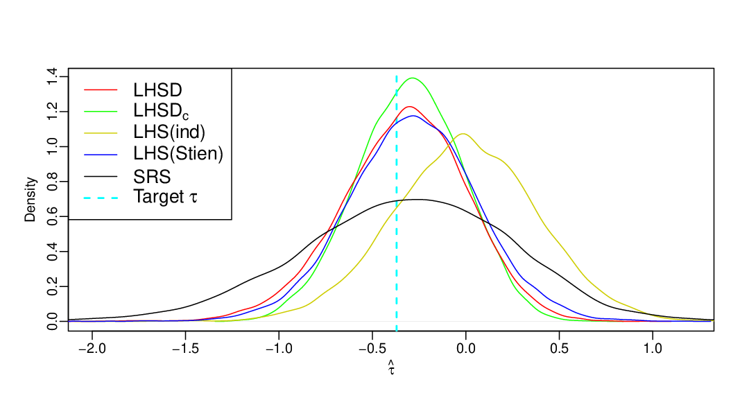
In this simulation study, the input variable is generated from a four-dimensional multivariate normal distribution . The parameters of the distribution, i.e. and , are randomly chosen, and then they are kept fixed for all replications. Here, is generated from the standard normal distribution. For the covariance matrix , first we generated a matrix from the standard normal distribution, then we took . We have generated random samples using five different methods – (i) LHSD: LHS using our proposed method given in Algorithm 2, (ii) : centered LHSD as proposed in Section 2.2.1, (iii) LHS(ind): LHS assuming that the components of are independent as given in Section 2.1, (iv) LHS(Stien): rank-based LHS proposed by Stein, 1987 and (v) SRS: the simple random sample. We used a fixed sample of size in all five cases and replicated the simulations times. We are interested in estimating , where
| (4.3) |
and . We estimate by using these five sampling procedures. The empirical densities of are plotted in Figure 1. We also repeated the experiment by taking sample sizes as , , and . The bias, variance and MSE of for all the five sampling methods are presented in Table 1. The true value of is calculated based on a SRS of size . The results show that LHS(ind) has a large bias, as it ignores the dependency structure among the components of . All other methods give very small bias. The variance of the SRS is very large, and for this reason, the MSE is also very large. On the other hand, our LHSD-based methods give the lowest MSE among all the methods. As mentioned in the previous section, the centered LHSD introduces a small bias, but it substantially reduces the variance of the estimator. As a result, it outperforms the other sampling schemes.
| Methods | Bias | Variance | MSE | Bias | Variance | MSE |
|---|---|---|---|---|---|---|
| LHSD | 0.08 | 10.55 | 10.56 | 0.03 | 10.22 | 10.22 |
| -0.20 | 7.19 | 7.23 | -0.15 | 8.24 | 8.26 | |
| LHS(ind) | -6.59 | 21.24 | 64.61 | -8.15 | 21.03 | 87.45 |
| LHS(Stien) | -0.39 | 13.06 | 13.21 | -0.22 | 12.81 | 12.86 |
| SRS | -0.03 | 16.50 | 16.50 | 0.12 | 16.75 | 16.77 |
| Methods | ||||||
| LHSD | 0.04 | 9.18 | 9.18 | -0.42 | 9.09 | 9.27 |
| -0.09 | 8.25 | 8.26 | -0.56 | 8.10 | 8.42 | |
| LHS(ind) | -12.77 | 20.03 | 183.16 | -15.29 | 19.40 | 253.24 |
| LHS(Stien) | -0.24 | 11.96 | 12.02 | -0.60 | 12.13 | 12.49 |
| SRS | -0.06 | 16.55 | 16.55 | -0.41 | 16.64 | 16.81 |
Table 1 shows that the bias and variance of for the LHSD are stable as the sample size increases, so it demonstrates that the estimator is -consistent as proved in Theorem 3.7. We also calculated the theoretical variances of the LHSD and SRS methods using equations (3.5) and (3.6), respectively, for sample size . We generated a large SRS of size and estimated and as discussed at the end of Section 3. The k-nearest neighbor algorithm is used in the non-parametric regression. The theoretical variances of for the LHSD and SRS are obtained as and , respectively. These values are also very close to the simulation results as given in Table 1.
| Methods | Mean | Variance | Mean | Variance |
|---|---|---|---|---|
| LHSD | 13.372 | 0.067 | 12.962 | 0.034 |
| 13.190 | 0.022 | 12.843 | 0.014 | |
| LHS(ind) | 59.854 | 138.219 | 59.742 | 89.030 |
| LHS(Stien) | 17.115 | 3.746 | 15.592 | 1.546 |
| SRS | 13.114 | 0.511 | 12.760 | 0.328 |
| Methods | ||||
| LHSD | 12.287 | 0.009 | 12.123 | 0.006 |
| 12.237 | 0.006 | 12.085 | 0.005 | |
| LHS(ind) | 59.299 | 33.388 | 59.118 | 23.950 |
| LHS(Stien) | 13.464 | 0.247 | 13.037 | 0.148 |
| SRS | 12.156 | 0.126 | 12.016 | 0.093 |
Now, we present a comparison study to see how well the different sampling schemes represent the target distribution. We need a goodness-of-fit measure to calculate the deviation of a random sample from the target distribution . The Kullback-Leibler (KL) divergence is used for this purpose (Kullback and Leibler, 1951). Suppose is the probability density function (p.d.f.) of the target distribution, and is the empirical p.d.f. Then, the KL-divergence between two densities is defined as
| (4.4) |
The first term in equation (4.4) is called the Shannon entropy function, which is estimated using ‘entropy’ function of ‘KNN’ package in R. The second term in equation (4.4) is simply estimated by . A small value of the KL-divergence indicates that the densities and are close to each other. If the two densities are identical, then the KL-divergence is zero, otherwise, it is always positive. The mean and variance of the KL-divergence over 10,000 replications are presented in Table 2 for different sample sizes. The SRS gives the minimum mean, as it generates unbiased random samples from the target distribution. Our LHSD-based sampling schemes are also giving the mean KL-divergence very close to the SRS, and their variances are around ten times smaller than the SRS. The mean from the rank based LHS method is very high for the small sample sizes, which indicates that there is a large bias in sampling from the target distribution. We also noticed that the variance of the KL-divergence using rank based LHS is considerably high in this example.
4.2 LHS from a Bivariate Logistic Distribution
In this section, we assume that input variable follows the Gumbel’s bivariate logistic distribution, where the joint distribution function is given by
The marginal distribution of is given by , The corresponding bivariate copula function is given by , . Since the copula is well known, we use Algorithm 3 to sample from the joint distribution using LHSD. The conditional copula is given by . The samples from the joint distribution are obtained using the following steps.
- 1.
Using Algorithm 1, we generate , a LHS of size from whose components are from i.i.d. .
- 2.
For , the corresponding samples from the joint copula is given by
- •
- •
.
- •
- 3.
For the LHSD from is given by
We are interested in estimating , where We generate random samples using the same five methods discussed in the previous example. Here, we use in all five cases and replicate the simulations times. The empirical density functions of using these methods are presented in Figure 2. The biases and MSEs are given in Table 2 for four different sample sizes , 30, 75 and 100. It is seen that the centered LHSD performs best. The rank based LHS method and LHSD have similar performance, but LHSD is slightly better in terms of the MSE. The LHS assuming independence produced a very large bias, and the SRS produced a large variance as expected.
| Methods | Bias | Variance | MSE | Bias | Variance | MSE |
|---|---|---|---|---|---|---|
| LHSD | 0.24 | 3.74 | 3.79 | 0.22 | 3.42 | 3.46 |
| 0.43 | 2.29 | 2.47 | 0.39 | 2.38 | 2.53 | |
| LHS(ind) | 1.70 | 4.89 | 7.77 | 2.01 | 4.52 | 8.55 |
| LHS(Stien) | 0.50 | 3.70 | 3.95 | 0.48 | 3.61 | 3.84 |
| SRS | 0.26 | 9.74 | 9.81 | 0.26 | 9.67 | 9.74 |
| Methods | ||||||
| LHSD | -0.23 | 3.19 | 3.24 | 0.06 | 3.14 | 3.15 |
| -0.09 | 2.55 | 2.55 | 0.16 | 2.76 | 2.79 | |
| LHS(ind) | 2.61 | 4.45 | 11.24 | 3.33 | 4.38 | 15.45 |
| LHS(Stien) | -0.11 | 3.26 | 3.27 | 0.20 | 3.21 | 3.25 |
| SRS | -0.23 | 9.92 | 9.97 | 0.06 | 9.90 | 9.91 |
| Methods | Mean | Variance | Mean | Variance |
|---|---|---|---|---|
| LHSD | 7.732 | 0.033 | 7.682 | 0.016 |
| 7.635 | 0.007 | 7.617 | 0.004 | |
| LHS(ind) | 8.312 | 0.074 | 8.277 | 0.042 |
| LHS(Stien) | 7.828 | 0.093 | 7.757 | 0.058 |
| SRS | 7.564 | 0.294 | 7.531 | 0.195 |
| Methods | ||||
| LHSD | 7.639 | 0.004 | 7.636 | 0.003 |
| 7.615 | 0.002 | 7.617 | 0.002 | |
| LHS(ind) | 8.257 | 0.012 | 8.258 | 0.008 |
| LHS(Stien) | 7.681 | 0.022 | 7.673 | 0.017 |
| SRS | 7.536 | 0.078 | 7.536 | 0.057 |
Like the previous example, we also estimated the KL-divergence using equation (4.4). The result is shown in Table 4. On an average, the SRS produces the minimum KL-divergence as the sampling scheme is unbiased. Both LHSD and LHSDc gives slightly higher mean values than SRS, however they are lower than the independent LHS and the ranked based LHS methods. The variance of the KL-divergence using LHSDc method is very low compared to the other methods.
5 Real Data Example: River Flood Inundation
We now illustrate our sampling methodology for a real application related to the river flood inundation model (Iooss, 2011). The study case concerns an industrial site located near a river and protected from it by a dyke. When the river height exceeds one of the dyke, flooding occurs. The goal is to study the water level with respect to the dyke height. The model considered here is based on a crude simplification of the 1D hydro-dynamical equations of Saint Venant under assumptions of uniform and constant flow rate and large rectangular sections. It consists of an equation that involves the characteristics of the river stretch given by
| (5.1) | |||||
| (5.2) |
The model output is the maximal annual overflow (in meters) and is the maximal annual height of the river (in meters). The inputs of the model (8 inputs) together with their probability distributions are defined in Table 5. Among the input variables of the model, dyke height is a design parameter; its variation range corresponds to a design domain. The randomness of the other variables is due to their spatio-temporal variability, our ignorance of their true value or some inaccuracies of their estimation. The river flow model is illustrated in Figure 3.
| Input | Description | Unit | Probability distribution |
|---|---|---|---|
| Maximal annual flowrate | Truncated Gumbel on | ||
| Strickler coefficient | – | Truncated normal on | |
| River downstream level | m | Triangular | |
| River upstream level | m | Triangular | |
| Dyke height | m | Uniform | |
| Bank level | m | Triangular | |
| L | Length of the river stretch | m | Triangular |
| B | River width | m | Triangular |

From the previous studies it is concluded that the inputs maximal annual flow-rate () and Strickler coefficient () are correlated with correlation coefficient (see Chastaing et al., 2012). This correlation is admitted in real case as it is known that the friction coefficient increases with the flow rate. Similarly, the river downstream and river upstream level are known to be correlated with correlation coefficient . The correlation coefficient between the length of the river and breadth of the river are also known to be . The other input variables are assumed to be uncorrelated.
The quantity of interest is the mean maximal annual overflow . We compare our proposed LHSD-based methods with the SRS, LHS(ind), LHS(Stien) in estimating . Although the marginal distribution of the inputs are known, the joint distribution is not known. We construct a joint distribution using the multivariate normal copula with the known pairwise correlation coefficients as described in Section 2.2.2. The choice of such copula is appropriate here as it would retain the known correlation structure in the inputs. The multivariate normal copula function for variables is given by
| (5.3) |
where is the joint c.d.f. of the multivariate normal distribution with covariance matrix , and is the c.d.f. of a standard normal distribution. In this example, , and , where for , , and all other elements of are . As most of the components on the copula function are assumed to be independent and the dependency exists only pairwise, the conditional copulas is easily obtained using properties of the bivariate normal distribution. The inverse of such conditional distributions can also be obtained using the inverse of the univariate normal distribution. Hence, we use Algorithm 3 to sample from the inputs using LHSD. The same conditional copulas are used to sample from the joint distribution using the SRS, those are also used in the first step of rank based LHS method.
We sample observations from the inputs using all these five methods and computed the corresponding value of the outputs using (5.1). The value of is estimated by the sample mean of the outputs. We repeated this procedure times to estimate the bias and variance of the estimator using these five methods. We also repeated the experiment by taking sample sizes as , , and . The results are shown in Table 6. The empirical probability distributions of the estimators are shown in Figure 4. Here, the target value of is computed by sampling inputs using the SRS method. Our LHSD-based methods give the best results in terms of both bias and MSE of the estimator. It is interesting to observe that the variance of the estimator using the SRS is very high, and for that reason even the biased LHS(ind) gives a smaller MSE than the SRS.
| Methods | Bias | Variance | MSE | Bias | Variance | MSE |
|---|---|---|---|---|---|---|
| LHSD | 0.013 | 0.010 | 0.010 | 0.062 | 0.008 | 0.011 |
| 0.010 | 0.005 | 0.005 | 0.061 | 0.005 | 0.009 | |
| LHS(ind) | 0.240 | 0.018 | 0.076 | 0.339 | 0.014 | 0.129 |
| LHS(Stien) | 0.029 | 0.013 | 0.014 | 0.073 | 0.009 | 0.015 |
| SRS | 0.013 | 0.853 | 0.853 | 0.079 | 0.819 | 0.825 |
| Methods | ||||||
| LHSD | 0.017 | 0.006 | 0.006 | 0.002 | 0.005 | 0.005 |
| 0.017 | 0.005 | 0.005 | 0.002 | 0.005 | 0.005 | |
| LHS(ind) | 0.455 | 0.011 | 0.218 | 0.508 | 0.011 | 0.269 |
| LHS(Stien) | 0.028 | 0.006 | 0.007 | 0.010 | 0.006 | 0.006 |
| SRS | 0.030 | 0.860 | 0.861 | -0.006 | 0.822 | 0.822 |

The biases and MSE of the estimators for all pairwise correlation coefficients are also computed using the five sampling methods (see Table 7). The true correlation coefficients for the first three pairs in that table, i.e. , , and , are non-zero. The last column for both bias and MSE combines all other pairs where the variables are pairwise independent, and we reported the maximum absolute bias and MSE for those pairs. It shows that all methods except LHS(ind) estimate the correlation coefficient efficiently. The LHSD and LHSDc methods gives smaller bias and MSE for the correlation coefficient in comparison to the ranked based LHS method. However, combining other results, we observe that the centered LHSD produces the best samples to estimate the output mean.
| Methods | Bias | MSE | ||||||
|---|---|---|---|---|---|---|---|---|
| LHSD | -0.026 | -0.006 | -0.009 | 0.003 | 0.019 | 0.027 | 0.027 | 0.036 |
| -0.023 | -0.009 | -0.011 | 0.003 | 0.018 | 0.027 | 0.027 | 0.036 | |
| LHS(ind) | -0.502 | -0.297 | -0.300 | 0.003 | 0.286 | 0.123 | 0.125 | 0.036 |
| LHS(Stien) | -0.038 | -0.015 | -0.013 | 0.002 | 0.026 | 0.030 | 0.030 | 0.036 |
| SRS | -0.017 | -0.005 | -0.004 | 0.002 | 0.023 | 0.029 | 0.029 | 0.036 |
6 Conclusion
In this paper, we have presented some new sampling methods, based on Latin hypercube sampling, to estimate the mean of the output variable when the inputs are treated as random variables with dependent components. It is theoretically proved that the asymptotic variance of the estimator is smaller than that of the estimator based on the SRS. The simulation results show that our estimators outperform the SRS, and also give smaller mean squared errors than the existing LHS methods. The most advantage of our method is that it retains the exact joint distribution of the input variables. To the best of our knowledge, there does not exist any other sampling scheme based on the LHS that satisfies this property in case of dependent inputs.
References
- Chastaing et al., (2012) Chastaing, G., Gamboa, F., and Prieur, C. (2012). Generalized Hoeffding-Sobol decomposition for dependent variables – application to sensitivity analysis. Electron. J. Stat., 6:2420–2448.
- Conti et al., (2009) Conti, S., Gosling, J. P., Oakley, J. E., and O’Hagan, A. (2009). Gaussian process emulation of dynamic computer codes. Biometrika, 96(3):663–676.
- Fang et al., (2006) Fang, K.-T., Li, R., and Sudjianto, A. (2006). Design and modeling for computer experiments. Computer Science and Data Analysis Series. Chapman & Hall/CRC, Boca Raton, FL.
- Iman and Conover, (1980) Iman, R. L. and Conover, W. J. (1980). Small sample sensitivity analysis techniques for computer models, with an application to risk assessment. Comm. Statist. A—Theory Methods, 9(17):1749–1874.
- Iooss, (2011) Iooss, B. (2011). Revue sur l’analyse de sensibilité globale de modèles numériques. J. SFdS, 152(1):3–25.
- Kennedy and O’Hagan, (2001) Kennedy, M. C. and O’Hagan, A. (2001). Bayesian calibration of computer models. J. Roy. Statist. Soc. Ser. B, 63(3):425–464.
- Kullback and Leibler, (1951) Kullback, S. and Leibler, R. A. (1951). On information and sufficiency. Ann. Math. Statistics, 22:79–86.
- McKay et al., (1979) McKay, M. D., Beckman, R. J., and Conover, W. J. (1979). A comparison of three methods for selecting values of input variables in the analysis of output from a computer code. Technometrics, 21(2):239–245.
- Oakley and O’hagan, (2002) Oakley, J. and O’hagan, A. (2002). Bayesian inference for the uncertainty distribution of computer model outputs. Biometrika, 89(4):769–784.
- O’Hagan, (2006) O’Hagan, A. (2006). Bayesian analysis of computer code outputs: a tutorial. Reliability Engineering & System Safety, 91(10):1290–1300.
- Owen, (1992) Owen, A. B. (1992). A central limit theorem for Latin hypercube sampling. J. Roy. Statist. Soc. Ser. B, 54(2):541–551.
- Sacks et al., (1989) Sacks, J., Welch, W. J., Mitchell, T. J., and Wynn, H. P. (1989). Design and analysis of computer experiments. Statist. Sci., 4(4):409–435.
- Simpson et al., (2001) Simpson, T. W., Poplinski, J., Koch, P. N., and Allen, J. K. (2001). Metamodels for computer-based engineering design: survey and recommendations. Engineering with Computers, 17(2):129–150.
- Sklar, (1959) Sklar, M. (1959). Fonctions de repartition an dimensions et leurs marges. Publ. inst. statist. univ. Paris, 8:229–231.
- Stein, (1987) Stein, M. (1987). Large sample properties of simulations using Latin hypercube sampling. Technometrics, 29(2):143–151.
- Volkova et al., (2008) Volkova, E., Iooss, B., and Van Dorpe, F. (2008). Global sensitivity analysis for a numerical model of radionuclide migration from the rrc ‘Kurchatov Institute’ radwaste disposal site. Stochastic Environmental Research and Risk Assessment, 22(1):17–31.
Appendix
Proof of Theorem 3.5.
Suppose form a LHS from , where the components of are i.i.d. variables. Then, using the inverse transformation in Equation (3.1) we get
where form a LHSD from having a target distribution . For , we define
where denotes the greatest integer less than or equal to . Following McKay et al., 1979, the joint density of and can be written as
where for . If , then
Using and keeping only the first order terms in the expansion of the product, we get
| (6.1) |
Define . Using Equation (3.3) we have
| (6.2) |
If is Riemann integrable, one can show that
| (6.3) |
Combining Equations (6.1), (6.2) and (6.3) we have
| (6.4) |
Therefore
∎
Proof of Theorem 3.7.
From Theorem 3.5 we find that the asymptotic variance of is . As , it is enough to prove that the asymptotic distribution of is normal. We write
| (6.5) |
where
Theorem 3.5 shows that . Since , it shows that . Finally, the theorem follows from Lemma 2 of Owen, 1992 that proves is asymptotically normal under the LHS. ∎