Wave number-Explicit Analysis for Galerkin Discretizations of Lossy Helmholtz Problems

Jens M. Melenk Thanks: (melenk@tuwien.ac.at), Institut für Analysis und Scientific Computing, Technische Universität Wien, Wiedner Hauptstrasse 8-10, A-1040 Wien, Austria. Stefan A. Sauter Thanks: (stas@math.uzh.ch), Institut für Mathematik, Universität Zürich, Winterthurerstr 190, CH-8057 Zürich, Switzerland Céline Torres Thanks: (celine.torres@math.uzh.ch), Institut für Mathematik, Universität Zürich, Winterthurerstr 190, CH-8057 Zürich, Switzerland

Abstract

We present a stability and convergence theory for the lossy Helmholtz equation and its Galerkin discretization. The boundary conditions are of Robin type. All estimates are explicit with respect to the real and imaginary part of the complex wave number $\zeta\in\mathbb{C}$ , $\operatorname{Re}\zeta\geq 0$ , $\left|\zeta\right|\geq 1$ . For the extreme cases $\zeta\in\operatorname*{i}\mathbb{R}$ and $\zeta\in\mathbb{R}_{\geq 0}$ , the estimates coincide with the existing estimates in the literature and exhibit a seamless transition between these cases in the right complex half plane.

1 Introduction

For many problems in time-harmonic acoustic scattering, the Helmholtz equation serves as a model problem, and its numerical discretization is a topic of vivid research. For homogeneous, isotropic material the differential operator is given by

\mathcal{L}_{\zeta}u:=-\Delta u+\zeta^{2}u,

where $\zeta=\operatorname{Re}\zeta+\operatorname{i}\operatorname{Im}\zeta=:\nu-k\operatorname{i}$ with $\nu>0$ and $k\in{\mathbb{R}}$ denotes the wave number. The solution is highly oscillatory if $\left|\operatorname{Im}\zeta\right|\gg 1$ , which makes the discretization challenging with respect to both, stability and accuracy. To study this problem systematically the case of purely imaginary wave numbers $\zeta=-\operatorname*{i}k$ , $k\in\mathbb{R}$ , has often been used in the literature as a model problem for designing and analyzing numerical methods. However, in many applications waves are damped, e.g., by friction and viscoelastic effects in the material or loss via sound radiation or flow of vibration energy out of the physical scatterer (see, e.g., [18]).

Another important application is the approximation of the inverse Laplace transform by contour quadrature where the Helmholtz operator has to be discretized at many complex frequencies in the right complex half plane (see, e.g., [5]).

For the two extreme cases $\zeta=-\operatorname*{i}k$ and $\zeta=\nu$ , $k\in\mathbb{R}$ , $\nu\in\mathbb{R}_{\geq 0}$ , a fairly complete theory for standard Galerkin $hp$ -finite elements is available and the error estimates are explicit with respect to the wave number $\zeta$ , the mesh width $h$ of the finite element mesh, and the polynomial degree $p$ : a) For $\zeta=-\operatorname*{i}k$ and large $\left|k\right|$ the problem is highly indefinite and a “resolution condition” of the form

\frac{|k|h}{p}\leq C\quad\text{ together with }\quad p\geq C\log\left|k\right|

has to be imposed in order to ensure solvability of the Galerkin equations and quasi-optimality ([9, 10, 8, 2]); b) for $\zeta=\nu>0$ and $\nu=O\left(1\right)$ , the problem is properly elliptic and Céa’s lemma ensures well-posedness and quasi-optimality without any resolution condition; c) for $\zeta=\nu\gg 1$ , the solution exhibits boundary layers. Although the Galerkin discretization is always well-posed in this last situation, special meshes should be used that are adapted to the boundary layers (see, e.g., [11, 16, 7] and references there). In this paper, we will develop a unified theory for Galerkin discretizations of $\mathcal{L}_{\zeta}$ with Robin boundary conditions that is applicable for all $\zeta\in\mathbb{C}$ , $\operatorname{Re}\zeta\geq 0$ , and $\left|\zeta\right|\geq 1$ . All estimates are explicit in terms of $\operatorname{Re}\zeta$ and $\operatorname{Im}\zeta$ and reproduce the limiting cases of purely real and imaginary $\zeta$ . It is shown that, for the sectorial case, i.e., the wave number lies in a sectorial neighborhood of the real axis in the right complex half plane, well-posedness and quasi-optimality is a consequence of coercivity while for $\operatorname{Re}\zeta\rightarrow 0$ the estimates tend continuously to the purely imaginary case $\zeta=-\operatorname*{i}k$ . We follow the general theory developed in [9, 10] and refine the estimates to be explicit with respect to the real and imaginary part of the wave number.

The paper is structured as follows. In Sect. 2 we introduce the Helmholtz model problem with Robin boundary conditions and formulate some geometric and algebraic assumptions on the data. Further, we define for the wave number the (well-behaved) sectorial and the (more critical) non-sectorial region.

The estimate of the continuity constant for the sesquilinear form is derived in Sect. 3. Sect. 4 is devoted to the analysis of the inf-sup constant for the continuous sesquilinear form. If the real part of the wave number is positive the estimate follows simply from the coercivity of the sesquilinear form. However, this bound degenerates as $\operatorname{Re}\zeta\rightarrow 0$ . This can be remedied by a different proof: first one uses suitable test functions to derive stability estimates for an adjoint problem with $L^{2}$ right-hand sides and then by employing this result for the estimate of the inf-sup constant in a vicinity of the imaginary axis.

The key role for the analysis of the Galerkin discretization is played by a regular decomposition of the Helmholtz solution. In Sect. 5, we introduce a splitting of the Helmholtz solution into a part with (low) $H^{2}$ -regularity and wave number-independent regularity constant and an analytic part with a more critical wave number dependence. First, this is derived for the full space solution by generalizing the results for purely imaginary frequencies in [9]. In the case of bounded domains, we generalize the iteration argument in [10, Sect. 4] to general complex frequencies. In addition, this requires sharp estimates of frequency-depending lifting operators which we also present in this section.

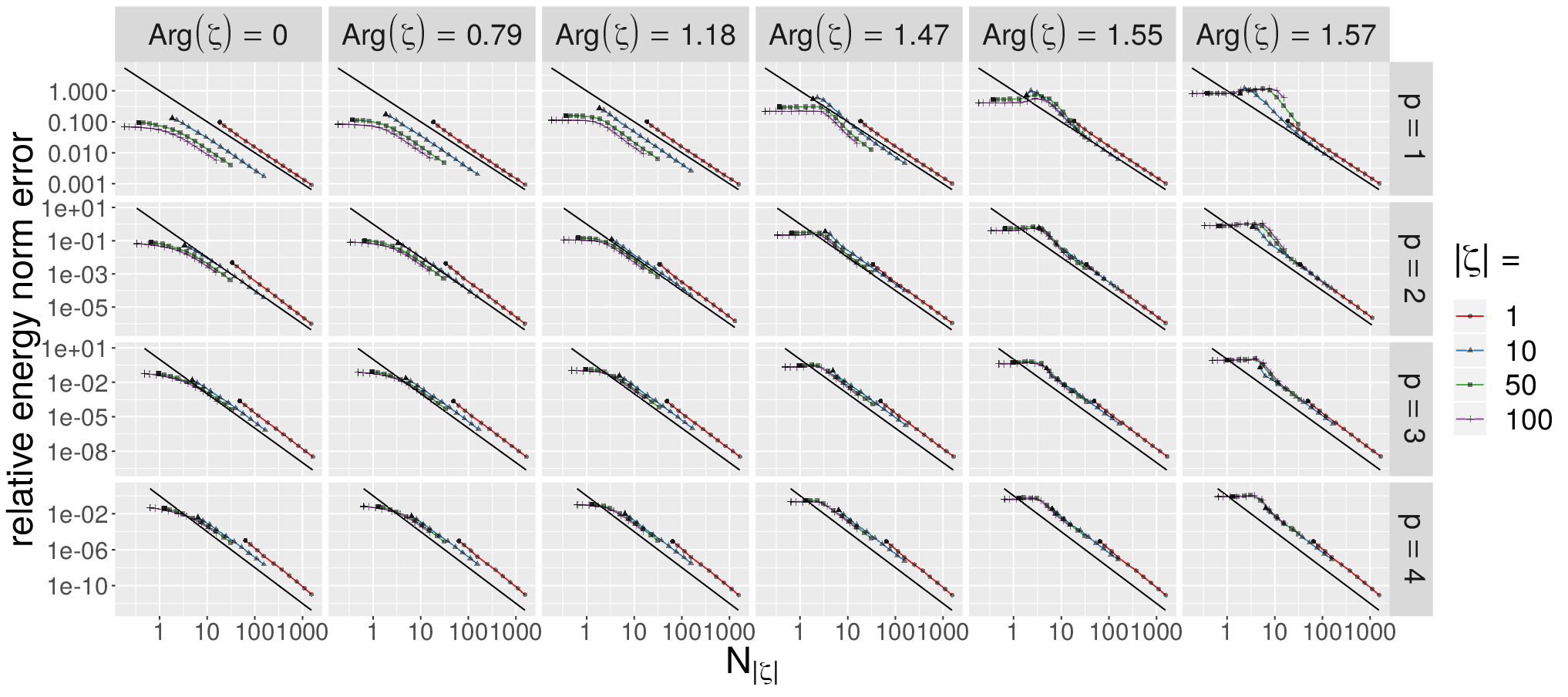
Sect. 6 is devoted to the estimate of the discrete inf-sup constant for the standard Galerkin discretization of the Helmholtz equation. We will derive two type of estimates: one requires that the finite dimensional space for the Galerkin discretization satisfies a certain resolution condition and allows for robust (as $\operatorname{Re}\zeta\rightarrow 0)$ stability and quasi-optimal convergence estimates; the other one avoids a resolution condition while the constants in the estimates tend towards $\infty$ as $\operatorname{Re}\zeta\rightarrow 0$ but stay robust for the sectorial case. Numerical examples in Sect. 7 illustrate the application of our analysis in the context of $hp$ -FEM.

2 Setting

We consider the Helmholtz problem

\begin{split}-\Delta u+\zeta^{2}u&=f\qquad\text{ in }\Omega,\\ \partial_{n}u+\zeta u&=g\qquad\text{ on }\Gamma:=\partial\Omega,\end{split}

(2.1)

for $f\in L^{2}(\Omega)$ and $g\in L^{2}(\Gamma)$ . We assume that the wave number (frequency) $\zeta$ satisfies¹¹ 1 The condition $|\zeta|\geq 1$ can be replaced by $\left|\zeta\right|\geq\rho_{0}$ for any $\rho_{0}>0$ . However, the constants in our estimates, possibly, deteriorate as $\rho_{0}\rightarrow 0$ .

\zeta\in\mathbb{C}_{\geq 0}^{\circ}:=\left\{\zeta\in\mathbb{C}_{\geq 0}\mid|\zeta|\geq 1\right\},

(2.2)

where, for $\rho\in\mathbb{R}$ ,

\mathbb{C}_{>\rho}:=\left\{\xi\in\mathbb{C}\mid\operatorname{Re}\xi>\rho\right\}\quad\text{and\quad}\mathbb{C}_{\geq\rho}:=\left\{\xi\in\mathbb{C}\mid\operatorname{Re}\xi\geq\rho\right\}.

Note that the choice $\zeta=-\operatorname*{i}k$ leads to the standard Helmholtz case. The frequency domain $\mathbb{C}_{\geq 0}^{\circ}$ is split into the sectorial and non-sectorial cases

	$\displaystyle S_{\beta}$	$\displaystyle:=\{\xi\in\mathbb{C}_{\geq 0}^{\circ}:\left\|\operatorname{Im}\xi\right\|<\beta\operatorname{Re}\xi\},$
	$\displaystyle S_{\beta}^{c}$	$\displaystyle:=\{\xi\in\mathbb{C}_{\geq 0}^{\circ}:\left\|\operatorname{Im}\xi\right\|\geq\beta\operatorname{Re}\xi\}$

for some $\beta>0$ . Our focus is on the derivation of stability and error estimates that are explicit in the real and imaginary part of $\zeta$ but less on the development of a theory with minimal assumptions on the geometry of the domain. In this light we impose the following simplifying assumption.

Assumption 2.1

$\Omega\subset\mathbb{R}^{3}$ is a bounded domain with analytic boundary that is star-shaped with respect to a ball.

We note that our results can be extended to convex polygonal domains in a straightforward way following the arguments in [10].

Let $L^{2}\left(\Omega\right)$ denote the usual Lebesgue space with scalar product denoted by $\left(\cdot,\cdot\right)$ (complex conjugation is on the second argument) and norm $\|\cdot\|_{L^{2}(\Omega)}:=\left\|\cdot\right\|:=\left(\cdot,\cdot\right)^{1/2}$ . Let $V=H^{1}\left(\Omega\right)$ denote the usual Sobolev space and let $\gamma_{0}:H^{1}\left(\Omega\right)\rightarrow H^{1/2}\left(\Gamma\right)$ be the standard trace operator. We introduce the sesquilinear forms

a_{0,\zeta}\left(u,v\right):=\left(\nabla u,\nabla v\right)+\left(\zeta^{2}u,v\right)\qquad\forall u,v\in V,

and

b_{\zeta}\left(\gamma_{0}u,\gamma_{0}v\right):=\left(\zeta\gamma_{0}u,\gamma_{0}v\right)_{\Gamma}\qquad\forall u,v\in V,

where $\left(\cdot,\cdot\right)_{\Gamma}$ is the $L^{2}\left(\Gamma\right)$ scalar product.

The weak formulation of the Helmholtz problem with Robin boundary conditions (2.1) is given as follows: For $F=(f,\cdot)+(g,\gamma_{0}\cdot)_{\Gamma}\in V^{\prime}$ , we seek $u\in V$ such that

a_{\zeta}\left(u,v\right):=a_{0,\zeta}\left(u,v\right)+b_{\zeta}\left(\gamma_{0}u,\gamma_{0}v\right)=F\left(v\right)\quad\forall v\in V.

(2.3)

In the following, we will omit explicitly writing the trace operator $\gamma_{0}$ when it is clear that it is implied.

3 The Continuity Constant

In this section, we will estimate the continuity constant of the sesquilinear form $a_{\zeta}\left(\cdot,\cdot\right)$ . We equip the Sobolev space $V$ with the indexed norm $\left\|\cdot\right\|_{|\zeta|}$ , where, for $\rho>0$ , we set

\left\|u\right\|_{\rho,\Omega}=\left\|u\right\|_{\rho}:=\left(\left\|\nabla u\right\|^{2}+\rho^{2}\left\|u\right\|^{2}\right)^{1/2}.

(3.1)

More generally, for measurable subsets $T\subset\Omega$ we write

\|u\|_{\rho,T}:=\left(\|\nabla u\|^{2}_{L^{2}(T)}+\rho^{2}\|u\|^{2}_{L^{2}(T)}\right)^{1/2}

The $L^{2}$ -norm on $\Gamma$ is denoted by $\|\cdot\|_{\Gamma}$ . On $H^{1/2}(\Gamma)$ we introduce the weighted norm

\left\|g\right\|_{\Gamma,\rho}:=\left(\|g\|^{2}_{H^{1/2}(\Gamma)}+\rho\|g\|^{2}_{\Gamma}\right)^{1/2},

(3.2)

for $\rho>0$ .

Theorem 3.1

The sesquilinear form $a_{\zeta}$ is continuous and

\left|a_{\zeta}\left(u,v\right)\right|\leq\left(1+C_{b}\right)\left\|u\right\|_{|\zeta|}\left\|v\right\|_{|\zeta|}\quad\forall u,v\in H^{1}\left(\Omega\right)

(3.3)

with $C_{b}$ independent of $\zeta\in\mathbb{C}_{\geq 0}$ .

Proof. The continuity estimate for the sesquilinear form $b_{\zeta}\left(\cdot,\cdot\right)$ is a simple consequence of the multiplicative trace inequality (see [4, p.41, last formula])

\left\|\gamma_{0}u\right\|_{\Gamma}\leq C_{\operatorname*{trace}}\left\|u\right\|^{1/2}\left\|u\right\|_{H^{1}(\Omega)}^{1/2}.

(3.4)

Hence

\sqrt{|\zeta|}\left\|\gamma_{0}u\right\|_{L^{2}\left(\Gamma\right)}\leq C_{\mathrm{trace}}\left(\left|\zeta\right|\left\|u\right\|\right)^{1/2}\left\|u\right\|_{H^{1}(\Omega)}^{1/2}\leq C\left\|u\right\|_{\left|\zeta\right|},

(3.5)

which implies the continuity of $b_{\zeta}\left(\cdot,\cdot\right)$

\left|b_{\zeta}\left(\gamma_{0}u,\gamma_{0}v\right)\right|\leq C_{b}\left\|u\right\|_{\left|\zeta\right|}\left\|v\right\|_{\left|\zeta\right|}\qquad\forall u,v\in H^{1}\left(\Omega\right)

(3.6)

for a constant $C_{b}$ independent of $\zeta\in\mathbb{C}_{\geq 0}^{\circ}$ and $u$ , $v$ .

4 The Inf-Sup Constant of $a_{\zeta}\left(\cdot,\cdot\right)$

Our goal in this section is to estimate the inf-sup constant

\gamma_{\zeta}:=\inf_{u\in V}\sup_{v\in V}\frac{\left|a_{\zeta}\left(u,v\right)\right|}{\left\|u\right\|_{\left|\zeta\right|}\left\|v\right\|_{|\zeta|}},

(4.1)

which implies well-posedness of (2.3). This involves two different theoretical techniques: In Sect. 4.1 we consider the case $\operatorname{Re}\zeta>0$ and obtain estimates from the coercivity of the sesquilinear form. These estimates give stable bounds for the sectorial case but deteriorate as $\operatorname{Re}\zeta\rightarrow 0$ in the non-sectorial case. In Sect. 4.2 we employ the sesquilinear form with a suitably selected test function and obtain sharp estimates also for the non-sectorial case.

4.1 The Inf-Sup Constant for $\operatorname{Re}\zeta>0$

The estimate of the inf-sup constant in the following Lemma 4.1 is a direct consequence of the technique used in [1].

Lemma 4.1

Let $\Omega\subset\mathbb{R}^{3}$ be a bounded Lipschitz domain and let $\zeta\in\mathbb{C}_{>0}^{\circ}$ . Then the inf-sup constant $\gamma_{\zeta}$ of (4.1) for the sesquilinear form $a_{\zeta}\left(\cdot,\cdot\right)$ (cf. (2.3)) satisfies

\gamma_{\zeta}\geq\frac{\operatorname{Re}\zeta}{\left|\zeta\right|}.

(4.2)

For every $F\in V^{\prime}$ , problem (2.3) has a unique solution. In particular if there are $f\in L^{2}\left(\Omega\right)$ , $g\in L^{2}\left(\Gamma\right)$ such that $F\left(v\right)=\left(f,v\right)+\left(g,v\right)_{\Gamma}$ , then the solution $u$ satisfies

\left\|u\right\|_{|\zeta|}\leq\frac{1}{\operatorname{Re}\zeta}\left(\left\|f\right\|+C\sqrt{\left|\zeta\right|}\left\|g\right\|_{\Gamma}\right).

(4.3)

Proof. We follow the idea of the proof in [1]. We choose $v=\frac{\zeta}{|\zeta|}u$ . For the sesquilinear form with Robin boundary conditions we have

\operatorname{Re}a_{\zeta}\left(u,\frac{\zeta}{|\zeta|}u\right)=\frac{\operatorname{Re}\zeta}{|\zeta|}\left\|u\right\|_{|\zeta|}^{2}+\left|\zeta\right|\left\|u\right\|_{\Gamma}^{2}\geq\frac{\operatorname{Re}\zeta}{|\zeta|}\left\|u\right\|_{\left|\zeta\right|}^{2}.

The positivity of the inf-sup constant $\gamma_{\zeta}$ implies unique solvability (see, e.g., [12, Thm. 2.1.44]; the above argument can be used to show [12, (2.34b)]). We obtain

\left\|u\right\|_{|\zeta|}\leq\frac{\left|\zeta\right|}{\operatorname{Re}\zeta}\sup_{v\in H^{1}\left(\Omega\right)\backslash\left\{0\right\}}\frac{\left|F\left(v\right)\right|}{\left\|v\right\|_{\left|\zeta\right|}}\leq\frac{|\zeta|}{\operatorname{Re}\zeta}\left(\frac{\left\|f\right\|}{|\zeta|}+\left\|g\right\|_{L^{2}\left(\Gamma\right)}\sup_{v\in H^{1}\left(\Omega\right)\backslash\left\{0\right\}}\frac{\left\|v\right\|_{\Gamma}}{\left\|v\right\|_{|\zeta|}}\right).

A multiplicative trace inequality in the form of (3.5) leads to (4.3).

Lemma 4.2

Let $\Omega\subset\mathbb{R}^{3}$ be a smooth domain that is star-shaped with respect to a ball or let $\Omega$ be a convex polyhedron. Let the functional $F\in V^{\prime}$ be of the form $F\left(v\right)=\left(f,v\right)+\left(g,v\right)_{\Gamma}$ with $f\in L^{2}\left(\Omega\right)$ and $g\in L^{2}\left(\Gamma\right)$ . Then, problem (2.3) has a unique solution and satisfies

\|u\|_{|\zeta|}\leq C_{S}\left(\frac{1}{1+\operatorname*{Re}(\zeta)}\left\|f\right\|+\frac{1}{\sqrt{1+\operatorname*{Re}(\zeta)}}\left\|g\right\|_{\Gamma}\right)

(4.4)

for some $C_{S}$ independent of $\zeta\in\mathbb{C}_{\geq 0}^{\circ}$ .

Remark 4.3

In [3], a stability estimate is proved that is related to (4.4) if $\operatorname*{Re}\zeta$ is sufficiently small. For $\zeta\in S_{\beta}^{c}$ , the estimate (4.4) is non-degenerate for $\operatorname*{Re}\zeta\rightarrow 0$ in contrast to (4.2) and the result in [3].

Proof. Without loss of generality, we assume that $\Omega$ is star-shaped with respect to the origin. We will fix a parameter $\beta>1$ sufficiently large at the end of the proof. We distinguish between two cases.

Case a: $\zeta\in S_{\beta}$ . The condition $|\zeta|\geq 1$ leads to

\displaystyle\operatorname{Re}\zeta>\left(1+\beta^{2}\right)^{-1/2}|\zeta|\geq\left(1+\beta^{2}\right)^{-1/2}

(4.5)

and Lemma 4.1 becomes applicable:

\gamma_{\zeta}\geq\frac{\operatorname{Re}(\zeta)}{\left|\zeta\right|}\geq\frac{1}{\sqrt{1+\beta^{2}}},

which implies (4.4) for $\zeta\in S_{\beta}$ .

Case b: $\zeta\in S_{\beta}^{c}$ . For $\operatorname{Re}\zeta>0$ , existence and uniqueness follows from Lemma 4.1 while the well-posedness in the case $\operatorname{Re}\zeta=0$ is a consequence of [6, Prop. 8.1.3]. We write $\zeta=\operatorname*{Re}\zeta+\operatorname*{i}\operatorname*{Im}\zeta=:\nu-\operatorname*{i}k$ so that $\zeta\in S_{\beta}^{c}$ implies $\left|k\right|\geq\beta\nu$ for $\beta>1$ . First let $\nu\geq 1$ . We choose $v=\frac{\zeta}{|\zeta|}u$ and consider the real part of (2.3), which yields

\frac{\nu}{|\zeta|}\left\|\nabla u\right\|^{2}+\nu|\zeta|\|u\|^{2}+\left|\zeta\right|\left\|u\right\|_{\Gamma}^{2}\leq|(f,u)|+|(g,u)|.

(4.6)

Young’s inequality on the right-hand side leads to

|(f,u)|+|(g,u)|\leq\frac{1}{2\nu|\zeta|}\|f\|^{2}+\frac{\nu|\zeta|}{2}\|u\|^{2}+\frac{1}{2|\zeta|}\left\|g\right\|_{\Gamma}^{2}+\frac{|\zeta|}{2}|u|_{\Gamma}^{2}.

These two inequalities imply

\|\nabla u\|^{2}+\frac{|\zeta|^{2}}{2}\|u\|^{2}+\frac{|\zeta|^{2}}{2\nu}\|u\|_{\Gamma}^{2}\leq\frac{1}{2\nu^{2}}\|f\|^{2}+\frac{1}{2\nu}\|g\|_{\Gamma}^{2},

which is the desired (4.4) in view of $\nu\geq 1$ .

The proof for $\nu<1$ is essentially a repetition of the arguments in the proof of [6, Prop. 8.1.4] using the inequalities for three different test functions in (2.3) and Young’s inequality. For completeness, we show the relevant inequalities. The first test function is $v=u$ yielding, after taking the real part,

\|\nabla u\|^{2}-(k^{2}-\nu^{2})\|u\|^{2}+\nu\|u\|^{2}_{\Gamma}\leq|(f,u)|+|(g,u)_{\Gamma}|.

(4.7)

Next we choose $v=-\operatorname*{sign}(k)u$ and consider the imaginary part to get

2|k|\nu\|u\|^{2}+|k|\|u\|_{\Gamma}^{2}\leq|(f,u)|+|(g,u)_{\Gamma}|.

(4.8)

As a last test function we use $v\left(x\right)=\left\langle x,\nabla u\left(x\right)\right\rangle$ ; note that the assumptions on the domain imply via elliptic regularity theory that $v\in V$ . Integration by parts yields with $d=3$ (we write $d$ to indicate the generalization to arbitrary spatial dimension $d$ )

	$\displaystyle\operatorname{Re}a_{\zeta}\left(u,v\right)$	$\displaystyle=\operatorname{Re}\left(\left(\nabla u,\nabla\left\langle x,\nabla u\right\rangle\right)+\zeta^{2}\left(u,\left\langle x,\nabla u\right\rangle\right)+\zeta\left(u,\left\langle x,\nabla u\right\rangle\right)_{\Gamma}\right)$
		$\displaystyle=\left\\|\nabla u\right\\|^{2}+\frac{1}{2}\left(x,\nabla\left(\left\\|\nabla u\right\\|^{2}\right)\right)+\operatorname{Re}\left(\zeta^{2}\left(u,\left\langle x,\nabla u\right\rangle\right)+\zeta\left(u,\left\langle x,\nabla u\right\rangle\right)_{\Gamma}\right)$
		$\displaystyle=\left(1-\frac{d}{2}\right)\left\\|\nabla u\right\\|^{2}+\frac{1}{2}\left(\left\langle x,n\right\rangle,\left\\|\nabla u\right\\|^{2}\right)_{\Gamma}+\frac{d\left(k^{2}-\nu^{2}\right)}{2}\left\\|u\right\\|^{2}$
		$\displaystyle+\frac{\left(\nu^{2}-k^{2}\right)}{2}\left(\left\langle x,n\right\rangle u,u\right)_{\Gamma}+\operatorname{Re}\left(\zeta\left(u,\left\langle x,\nabla u\right\rangle\right)_{\Gamma}\right)+2\nu k\operatorname{Im}\left(u,\left\langle x,\nabla u\right\rangle\right)$
		$\displaystyle\leq\|(f,\left\langle x,\nabla u\left(x\right)\right\rangle)\|+\|(g,\left\langle x,\nabla u\left(x\right)\right\rangle)_{\Gamma}\|.$

Rearranging yields

		$\displaystyle\frac{d(k^{2}-\nu^{2})}{2}\\|u\\|^{2}+\frac{1}{2}(\langle x,n\rangle,\|\nabla u\|^{2})_{\Gamma}\leq\left(\frac{d}{2}-1\right)\\|\nabla u\\|^{2}+\frac{k^{2}}{2}(\langle x,n\rangle\|u\|^{2})_{\Gamma}$		(4.9)
		$\displaystyle+\|\zeta\|\\|u\\|_{\Gamma}\\|\langle x,\nabla u\rangle\\|_{\Gamma}+2\nu k\\|u\\|\\|\langle x,\nabla u\rangle\\|+\|(f,\langle x,\nabla u\rangle)\|+\|(g,\langle x,\nabla u\rangle)_{\Gamma}\|.$

We remark that (4.8) and (4.7) give

	$\displaystyle k\\|u\\|^{2}_{\Gamma}$	$\displaystyle\stackrel{{\scriptstyle\eqref{eq:11b}}}{{\leq}}\|(f,u)\|+\\|g\\|_{\Gamma}\\|u\\|_{\Gamma}\leq\|(f,u)\|+\frac{1}{2k}\\|g\\|^{2}_{\Gamma}+\frac{k}{2}\\|u\\|^{2}_{\Gamma},$		(4.10)
	$\displaystyle\\|\nabla u\\|^{2}$	$\displaystyle\leq(k^{2}-\nu^{2})\\|u\\|^{2}+\|(f,u)\|+\|(g,u)_{\Gamma}\|,$		(4.11)

which allows for controlling $\|u\|_{\Gamma}$ and $\|\nabla u\|$ in terms of $k\|u\|$ and the data $f$ , $g$ :

	$\displaystyle k\\|u\\|^{2}_{\Gamma}$	$\displaystyle\leq\frac{2}{k}\\|f\\|(k\\|u\\|)+\frac{1}{k}\\|g\\|^{2}_{\Gamma},$		(4.12)
	$\displaystyle\\|\nabla u\\|^{2}$	$\displaystyle\leq(k^{2}-\nu^{2})\\|u\\|^{2}+\frac{3}{k}\\|f\\|(k\\|u\\|)+\frac{2}{k}\\|g\\|^{2}_{\Gamma}.$		(4.13)

Since $\Omega$ is assumed to be star-shaped, one has $0<c_{1}\leq\langle x,n(x)\rangle\leq c_{2}$ for all $x\in\Gamma$ . Inserting this and (4.13) into (4.9) gives with $c_{3}=\operatorname{diam}\Omega$

		$\displaystyle(k^{2}-\nu^{2})\\|u\\|^{2}+\frac{c_{1}}{2}\\|\nabla u\\|^{2}_{\Gamma}\leq k^{2}\frac{c_{2}}{2}\\|u\\|^{2}_{\Gamma}+\left(\frac{d}{2}-1\right)\left(\frac{3}{k}\\|f\\|k\\|u\\|+\frac{2}{k}\\|g\\|^{2}_{\Gamma}\right)$
		$\displaystyle+\|\zeta\|\\|u\\|_{\Gamma}\\|\langle x,\nabla u\rangle\\|_{\Gamma}+2\nu k\\|u\\|\\|\langle x,\nabla u\rangle\\|+\|(f,\langle x,\nabla u\rangle)\|+\|(g,\langle x,\nabla u\rangle)_{\Gamma}\|.$

The proof can be completed with suitable applications of Young’s inequality, use of (4.12), (4.13), and selecting $\beta$ sufficiently large to treat the term $\nu k\|u\|\|\langle x,\nabla u\rangle\|\leq c_{3}\nu k\|u\|\|\nabla u\|$ .

4.2 The Inf-Sup Constant of $a_{\zeta}\left(\cdot,\cdot\right)$ for $\zeta\in S_{\beta}^{c}$

In the following Theorem 4.4 we will prove an alternative estimate (compared to (4.2)) for the inf-sup constant that is robust as $\operatorname{Re}\zeta\rightarrow 0$ . To estimate this constant we employ the standard ansatz $u\in V$ and $v=u+z$ for some $z\in V$ . Then

a_{\zeta}\left(u,u+z\right)=\left\|u\right\|_{\left|\zeta\right|}^{2}+a_{\zeta}\left(u,z\right)+b_{\zeta}\left(\gamma_{0}u,\gamma_{0}u\right)+\left(\zeta^{2}-\left|\zeta\right|^{2}\right)\left\|u\right\|^{2}.

The choice of $z$ will be related to some adjoint problem.the next section.

Theorem 4.4

Let $\Omega\subset\mathbb{R}^{3}$ be a smooth domain that is star-shaped with respect to a ball or let $\Omega$ be a convex polyhedron. Then there exists a constant $c>0$ such that for all $\zeta\in\mathbb{C}_{\geq 0}^{\circ}$ the inf-sup constant $\gamma_{f}$ of (4.1) satisfies

\gamma_{\zeta}\geq\frac{1}{1+c\frac{\left|\operatorname{Im}\zeta\right|}{1+\operatorname{Re}\zeta}}.

Proof. Let $\nu=\operatorname{Re}\zeta$ and $k=-\operatorname{Im}\zeta$ and set $\sigma=1/\sqrt{2}$ . First, we consider the case $\zeta\in\mathbb{C}_{\geq 0}^{\circ}$ with $\nu\geq\sigma$ .

From Lemma 4.1 we have for any $\zeta\in\mathbb{C}_{\geq\sigma}^{\circ}$ the estimate

\gamma_{\zeta}\geq\frac{\operatorname{Re}\zeta}{\left|\zeta\right|}=\frac{1}{\sqrt{1+\left(\frac{k}{\nu}\right)^{2}}}\geq\frac{1}{1+\frac{\left|k\right|}{\nu}}\geq\frac{1}{1+c\frac{\left|k\right|}{\nu+1}}\quad\text{for }c=1+\sqrt{2}.

It remains to consider the case $\zeta\in\mathbb{C}_{\geq 0}^{\circ}$ with $\nu<\sigma$ . Let $u,z\in V$ and set $v=u+z$ . Then

a_{\zeta}\left(u,v\right)=\left\|u\right\|_{\left|\zeta\right|}^{2}+\left(\zeta^{2}-\left|\zeta\right|^{2}\right)\left\|u\right\|^{2}+\zeta\left(u,u\right)_{\Gamma}+a_{\zeta}\left(u,z\right).

(4.14)

We consider the adjoint problem: find $z\in V$ such that

a_{\overline{\zeta}}\left(z,w\right)=\alpha^{2}\left(u,w\right)\quad\forall w\in V\quad\text{with\quad}\alpha^{2}:=\left|\zeta\right|^{2}-\overline{\zeta}^{2}=-2k\operatorname*{i}\overline{\zeta},

(4.15)

which is well-posed according to Lemma 4.2 and satisfies

\left\|z\right\|_{|\zeta|}\leq C_{S}\left|\alpha\right|^{2}\left\|u\right\|=2C_{S}\left|k\zeta\right|\left\|u\right\|\leq 2C_{S}\left|k\right|\left\|u\right\|_{|\zeta|}.

For this choice of $z$ , we consider the real part of (4.14) and obtain

\operatorname{Re}a_{\zeta}\left(u,v\right)\geq\left\|u\right\|_{|\zeta|}^{2}+\nu\left\|u\right\|_{\Gamma}^{2}\geq\left\|u\right\|_{|\zeta|}^{2}.

Hence

\left\|v\right\|_{|\zeta|}\leq\left(1+2C_{S}\left|k\right|\right)\left\|u\right\|_{|\zeta|}

and

\gamma_{\zeta}\geq\frac{1}{1+2C_{S}\left|k\right|}\geq\frac{1}{1+\tilde{c}\frac{\left|k\right|}{\nu+1}}\quad\text{for }0\leq\nu\leq\sigma.

5 Regular Decomposition of the Helmholtz Solution

In this section, we develop a regular decomposition of the solution of the Helmholtz problem (2.1) based on a frequency splitting of the right-hand side. The frequency splitting for functions defined on the full space $\mathbb{R}^{3}$ is defined via their Fourier transform (Sect. 5.1). For functions defined on finite domains, we derive the regular splitting using a lifting operator (Sect. 5.3). This generalizes the theory developed in [9, 10] to complex frequencies and the resulting estimates are explicit with respect to the real and imaginary part of the wave number.

5.1 The Full Space Adjoint Problem for $\zeta\in S_{\beta}^{c}$

The first result concerns the adjoint problem for the full space $\Omega=\mathbb{R}^{3}$ . Let $\phi\in L^{2}\left(\Omega\right)$ be a function with compact support. We choose $R>0$ sufficiently large so that the open ball $B_{R}$ with radius $R$ centered at the origin contains $\operatorname*{supp}\phi$ . We consider the problem

\begin{split}(-\Delta+\overline{\zeta^{2}})z&=\phi\qquad\qquad\text{ in }\mathbb{R}^{3},\\ \left|\left\langle\frac{x}{\left\|x\right\|},\nabla z\left(x\right)\right\rangle+\overline{\zeta}z\left(x\right)\right|&=o\left(\|x\|^{-1}\right)~\text{ as }\|x\|\rightarrow\infty.\end{split}

(5.1)

To analyze this equation we employ Fourier transformation and introduce a cutoff function $\mu\in C^{\infty}\left(\mathbb{R}_{\geq 0}\right)$ satisfying :w

\begin{array}[c]{lll}\operatorname*{supp}\mu\subset\left[0,4R\right],&\left.\mu\right|_{\left[0,2R\right]}=1,&\left|\mu\right|_{W^{1,\infty}\left(\mathbb{R}_{\geq 0}\right)}\leq\dfrac{C_{\mu}}{R},\\ &&\\ \forall x\in\mathbb{R}_{\geq 0}:0\leq\mu\left(x\right)\leq 1,&\left.\mu\right|_{\left[4R,\infty\right[}=0,&\left|\mu\right|_{W^{2,\infty}\left(\mathbb{R}_{\geq 0}\right)}\leq\dfrac{C_{\mu}}{R^{2}}.\end{array}

(5.2)

The fundamental solution to the Helmholtz operator $\mathcal{L}_{\zeta}u=-\Delta u+\zeta^{2}u$ in $\mathbb{R}^{3}$ is given by

G\left(\zeta,x\right):=g\left(\zeta,\left\|x\right\|\right)\quad\text{with\quad}g\left(\zeta,r\right):=\frac{\operatorname*{e}^{-\zeta r}}{4\pi r}.

It satisfies

\left|\left\langle\frac{x}{\left\|x\right\|},\nabla_{x}G\left(\zeta,x\right)\right\rangle+\zeta G\left(\zeta,x\right)\right|=o\left(\left\|x\right\|^{-1}\right)\quad\text{for }\left\|x\right\|\rightarrow\infty

so that $z$ is given by $z=G(\overline{\zeta})\ast\phi$ . Define $M\left(x\right):=\mu\left(\left\|x\right\|\right)$ and

z_{\mu}\left(x\right):=\left(G\left(\overline{\zeta}\right)M\right)\ast\phi:=\int_{B_{R}}G\left(\overline{\zeta},x-y\right)M\left(x-y\right)\phi\left(y\right)dy\qquad\forall x\in\mathbb{R}^{3}.

The properties of $\mu$ ensure $z_{\mu}|_{B_{R}}=z|_{B_{R}}$ . To analyze the stability and regularity of $z_{\mu}$ we introduce a frequency splitting of the solution $z_{\mu}=z_{H^{2}}+z_{{\mathcal{A}}}$ that depends on the complex frequency $\zeta\in\mathbb{C}_{\geq 0}$ and a parameter $\lambda\geq\lambda_{0}>1$ .

Lemma 5.1

Let $\phi\in L^{2}\left(\mathbb{R}^{3}\right)$ such that $\operatorname*{supp}\phi$ is contained in a ball $B_{R}:=B_{R}(0)$ of radius $R>0$ centered at the origin, and let $\mu$ be a cutoff function satisfying (5.2). Then there exists a constant $C>0$ depending only on $R$ and $\mu$ such that the solution $z=G\left(\overline{\zeta}\right)\ast\phi$ of (5.1) and $z_{\mu}:=\left(G\left(\overline{\zeta}\right)M\right)\ast\phi$ satisfy $\left.z\right|_{B_{R}}=\left.z_{\mu}\right|_{B_{R}}$ and

\left\|z_{\mu}\right\|_{|\zeta|}\leq\frac{C}{1+\operatorname{Re}\zeta}\|\phi\|\qquad\forall\zeta\in\mathbb{C}_{\geq 0}.

(5.3)

Furthermore, for every $\lambda\geq\lambda_{0}>1$ and $\zeta\in\mathbb{C}_{\geq 0}$ with $\operatorname{Im}\zeta\neq 0$ there exists a $\lambda$ - and $\zeta$ -dependent splitting $z_{\mu}=z_{H^{2}}+z_{{\mathcal{A}}}$ satisfying

	$\displaystyle\left\\|\nabla^{p}z_{H^{2}}\right\\|$	$\displaystyle\leq C^{\prime}\frac{\lambda}{\lambda-1}\left(\frac{\|\zeta\|}{\operatorname{Im}\zeta}\right)^{2}\left(\lambda\left\|\operatorname{Im}\zeta\right\|\right)^{p-2}\left\\|\phi\right\\|\qquad\forall p\in\{0,1,2\},$		(5.5)
	$\displaystyle\\|\nabla^{p}z_{{\mathcal{A}}}\\|$	$\displaystyle\leq C^{\prime}\frac{1+\left\|\zeta\right\|}{1+\operatorname{Re}\zeta}\left(\sqrt{3}\lambda\left\|\operatorname{Im}\zeta\right\|\right)^{p-2}\left\\|\phi\right\\|\qquad\forall p\in{\mathbb{N}}_{0}.$		(5.6)

Here, $|\nabla^{p}z_{\mathcal{A}}|$ stands for a sum over all derivatives of order $p$ (see (5.16)). The constant $C^{\prime}$ depends only on $\lambda_{0}$ , $R$ , and $\mu$ .

Remark 5.2

As the estimates in Lemma 5.1 degenerate for $\operatorname{Im}\zeta\rightarrow 0$ , we will employ Lemma 5.1 for $\zeta\in S^{c}_{\beta}$ for fixed $\beta>0$ . Then $\left|\operatorname{Im}\zeta\right|\geq\beta\operatorname{Re}\zeta$ and we have

\left|\operatorname{Im}\zeta\right|\leq\left|\zeta\right|\leq\tilde{C}\left|\operatorname{Im}\zeta\right|\quad\text{with\hskip 10.22217pt}\tilde{C}:=\frac{\sqrt{1+\beta^{2}}}{\beta}.

(5.7)

In particular, $\zeta\in S^{c}_{\beta}$ implies $\operatorname{Im}\zeta\neq 0$ .

Proof. For $\zeta\in\mathbb{C}_{\geq 0}$ , we set $\nu=\operatorname{Re}\zeta$ and $k=-\operatorname*{Im}\zeta$ . In order to construct the splitting $z=z_{H^{2}}+z_{\mathcal{A}}$ , we start by recalling the definition of the Fourier transformation for functions with compact support

\hat{w}\left(\xi\right)=\mathcal{F}\left(w\right)=\left(2\pi\right)^{-d/2}\int_{\mathbb{R}^{d}}\operatorname{e}^{-\operatorname*{i}\left\langle\xi,x\right\rangle}w\left(x\right)dx\qquad\forall\xi\in\mathbb{R}^{d}

and the inversion formula

w\left(x\right)=\mathcal{F}^{-1}\left(w\right)=\left(2\pi\right)^{-d/2}\int_{\mathbb{R}^{d}}\operatorname{e}^{\operatorname*{i}\left\langle x,\xi\right\rangle}\hat{w}\left(\xi\right)d\xi\qquad\forall x\in\mathbb{R}^{d}.

Next, we introduce a frequency splitting of a function $w\in L^{2}\left(\Omega\right)$ depending on $\zeta$ and a parameter $\lambda>1$ by using the Fourier transformation. The low- and high-frequency part of $w$ is given by

L_{\mathbb{R}^{3}}w:=\mathcal{F}^{-1}\left(\chi_{\lambda\left|k\right|}\mathcal{F}\left(w\right)\right)\quad\text{and\quad}H_{\mathbb{R}^{3}}w:=\mathcal{F}^{-1}\left(\left(1-\chi_{\lambda\left|k\right|}\right)\mathcal{F}\left(w\right)\right)

(5.8)

where $\chi_{\delta}$ is the characteristic function of the open ball with radius $\delta>0$ centered at the origin.

We construct a decomposition of $z_{\mu}$

z_{\mu}=z_{H^{2}}+z_{\mathcal{A}}.

(5.9)

as follows: We decompose the right-hand side $\phi$ in (5.1) via

\phi=\phi_{\left|k\right|}+\phi_{\left|k\right|}^{c}=L_{\mathbb{R}^{3}}\phi+H_{\mathbb{R}^{3}}\phi.

(5.10)

Accordingly, we define the decomposition of $z_{\mu}$ by

z_{H^{2}}:=\left(G\left(\overline{\zeta}\right)M\right)\star\phi_{\left|k\right|}^{c}\quad\text{and\quad}z_{{\mathcal{A}}}:=\left(G\left(\overline{\zeta}\right)M\right)\star\phi_{\left|k\right|}.

(5.11)

The Fourier transform of $G\left(\overline{\zeta},\cdot\right)M$ is given by

\left(\widehat{G\left(\overline{\zeta},\cdot\right)M}\right)\left(\xi\right)=\sigma\left(\overline{\zeta},\left\|\xi\right\|\right)

with

\sigma\left(\zeta,s\right)=(2\pi)^{-3/2}4\pi{\displaystyle\int_{0}^{\infty}}g\left(\zeta,r\right)\mu\left(r\right)r^{2}\dfrac{\sin\left(rs\right)}{rs}dr.

In the following we will analyze the symbol $\sigma\left(\zeta,\cdot\right)$ . We have:

	$\displaystyle\left\|s\sigma\left(\zeta,s\right)\right\|$	$\displaystyle=(2\pi)^{-3/2}\left\|{\displaystyle\int_{0}^{\infty}}\operatorname{e}^{-\zeta r}\mu\left(r\right)\sin\left(rs\right)dr\right\|$
		$\displaystyle\leq(2\pi)^{-3/2}\int_{0}^{4R}\operatorname*{e}\nolimits^{-\nu r}dr=4R\sqrt{\frac{2}{\pi}}E_{0}\left(4R\nu\right)$

with $E_{0}\left(t\right):=\frac{1-\operatorname*{e}\nolimits^{-t}}{t}\leq\frac{C_{0}}{1+t}.$ Applying integration by parts leads to

	$\displaystyle\sigma\left(\zeta,s\right)$	$\displaystyle=(2\pi)^{-3/2}{\displaystyle\int_{0}^{\infty}}\operatorname{e}^{-\zeta r}\mu\left(r\right)\dfrac{\sin\left(rs\right)}{s}dr$
		$\displaystyle=(2\pi)^{-3/2}\frac{1}{\zeta}{\displaystyle\int_{0}^{\infty}}\operatorname{e}^{-\zeta r}\partial_{r}\left(\mu\left(r\right)\dfrac{\sin\left(rs\right)}{s}\right)dr$
		$\displaystyle=(2\pi)^{-3/2}\frac{1}{\zeta}{\displaystyle\int_{0}^{\infty}}\operatorname{e}^{-\zeta r}\left(\mu^{\prime}\left(r\right)\dfrac{\sin\left(rs\right)}{s}+\mu\left(r\right)\cos rs\right)dr.$

This allows for the estimate

	$\displaystyle\left\|\sigma\left(\zeta,s\right)\right\|$	$\displaystyle=(2\pi)^{-3/2}\frac{1}{\|\zeta\|}\left\|{\displaystyle\int_{0}^{\infty}}\operatorname{e}^{-\zeta r}\left(\mu^{\prime}\left(r\right)\dfrac{\sin\left(rs\right)}{s}+\mu\left(r\right)\cos rs\right)dr\right\|$
		$\displaystyle\leq(2\pi)^{-3/2}\frac{1}{\|\zeta\|}{\displaystyle\int_{0}^{4R}}\operatorname{e}^{-\nu r}\left(\frac{C_{\mu}}{R}r+1\right)dr$
		$\displaystyle\leq 4R(2\pi)^{-3/2}\frac{1}{\|\zeta\|}\left(4C_{\mu}E_{1}\left(4\nu R\right)+E_{0}\left(4R\nu\right)\right)$

with

E_{1}\left(t\right)=\frac{1-\operatorname*{e}^{-t}(1+t)}{t^{2}}\leq E_{0}^{2}\left(t\right).

Hence,

\left|\sigma\left(\zeta,s\right)\right|\leq 4R(2\pi)^{-3/2}\frac{E_{0}\left(4R\nu\right)}{|\zeta|}\left(1+4C_{\mu}E_{0}(4R\nu)\right).

Since $E_{0}\left(t\right)\leq 1$ we end up with

\left|\sigma\left(\zeta,s\right)\right|\leq 4R\left(1+4C_{\mu}\right)(2\pi)^{-3/2}\frac{E_{0}\left(4R\nu\right)}{|\zeta|}.

As a consequence, we have proved that

	$\displaystyle\|\zeta\|\left\\|z_{\mu}\right\\|$	$\displaystyle\leq 4R\left(1+4C_{\mu}\right)E_{0}\left(4R\nu\right)\left\\|\phi\right\\|,$
	$\displaystyle\left\\|\partial_{i}z_{\mu}\right\\|$	$\displaystyle\leq 4RE_{0}\left(4R\nu\right)\left\\|\phi\right\\|$

so that we have

\left\|z_{\mu}\right\|_{|\zeta|}\leq\sqrt{2+\left(1+4C_{\mu}\right)^{2}}\left(16\pi R\right)E_{0}\left(4R\nu\right)\left\|\phi\right\|.

This shows (5.3). In the following we estimate higher order derivatives. For the product $s^{2}\sigma\left(s\right)$ , we get

	$\displaystyle\left\|s^{2}\sigma\left(\zeta,s\right)\right\|$	$\displaystyle=(2\pi)^{-3/2}\left\|\int_{0}^{\infty}\operatorname{e}^{-\zeta r}\mu\left(r\right)s\sin\left(rs\right)dr\right\|$
		$\displaystyle=(2\pi)^{-3/2}\left\|\int_{0}^{\infty}\operatorname{e}^{-\zeta r}\mu\left(r\right)\partial_{r}\cos\left(rs\right)dr\right\|$
		$\displaystyle\leq(2\pi)^{-3/2}\left(\left\|\int_{0}^{\infty}\cos\left(rs\right)\partial_{r}\left(\operatorname{e}^{-\zeta r}\mu\left(r\right)\right)dr\right\|+1\right)$
		$\displaystyle\leq(2\pi)^{-3/2}\|\zeta\|\left\|\int_{0}^{\infty}\cos\left(rs\right)\operatorname{e}^{-\zeta r}\mu\left(r\right)dr\right\|$
		$\displaystyle\quad+(2\pi)^{-3/2}\left(\left\|\int_{0}^{\infty}\cos\left(rs\right)\operatorname{e}^{-\nu r}\mu^{\prime}\left(r\right)dr\right\|+1\right)$
		$\displaystyle=:T^{\operatorname{I}}+T^{\operatorname{II}}.$

The estimates

	$\displaystyle T^{\operatorname*{I}}$	$\displaystyle\leq(2\pi)^{-3/2}4RE_{0}\left(4R\nu\right)\|\zeta\|,$		(5.12)
	$\displaystyle T^{\operatorname*{II}}$	$\displaystyle\leq(2\pi)^{-3/2}4CE_{0}\left(4R\nu\right)$		(5.13)

follow from the properties of $\mu$ (cf. (5.2)). As a simple consequence we obtain for $m\geq 2$

\left|s^{2}\sigma\left(\zeta,s\right)\right|\leq(2\pi)^{-3/2}4\left(C+R|\zeta|\right)E_{0}\left(4R\nu\right)

(5.14)

and

\sup_{0<s<\lambda\left|k\right|}\left|s^{m}\sigma\left(\zeta,s\right)\right|\leq(2\pi)^{-3/2}4\left(C+R|\zeta|\right)E_{0}\left(4R\nu\right)\left(\lambda\left|k\right|\right)^{m-2}.

(5.15)

Hence for $\alpha\in\mathbb{N}_{0}^{3}$ , $\left|\alpha\right|=2$ , we have

\left\|\partial^{\alpha}z_{\mu}\right\|\leq 4\left(R\left|\zeta\right|+C\right)E_{0}\left(4R\nu\right)\left\|\phi\right\|

and

	$\displaystyle\\|\nabla^{p}z_{{\mathcal{A}}}\\|$	$\displaystyle=\sqrt{\sum_{\begin{subarray}{c}\alpha\in\mathbb{N}_{0}^{3}\\ \left\|\alpha\right\|=p\end{subarray}}\binom{p}{\alpha}\left\\|\partial^{\alpha}z_{\mathcal{A}}\right\\|^{2}}\leq C^{\prime}E_{0}\left(4R\nu\right)\left(1+\left\|\zeta\right\|\right)\left(\lambda\left\|k\right\|\right)^{p-2}3^{p/2}\left\\|\phi\right\\|$
		$\displaystyle\leq C^{\prime\prime}\frac{1+\|\zeta\|}{1+\nu}\left(\sqrt{3}\lambda\left\|k\right\|\right)^{p-2}\left\\|\phi\right\\|\qquad\forall p\in{\mathbb{N}}_{\geq 2}.$		(5.16)

The bounds (5.16) expresses the desired estimate (5.6). A direct application of (5.14) does not lead to (5.5) as it introduces an undesired factor $|\zeta|$ . This is removed by noting that is suffices to consider $s=\|\xi\|$ with $s\geq\lambda|k|$ and that only the estimates for $T^{I}$ need to be refined. This is achieved with an integration by parts:

$\displaystyle\left\|T^{\operatorname*{I}}\right\|$	$\displaystyle=(2\pi)^{-3/2}\|\zeta\|\left\|\int_{0}^{4R}\cos\left(rs\right)\operatorname{e}^{-\zeta r}\mu\left(r\right)dr\right\|$
	$\displaystyle=(2\pi)^{-3/2}\|\zeta\|\left\|\left(\frac{\zeta}{\zeta^{2}+s^{2}}+\int_{0}^{4R}\frac{\operatorname*{e}^{-\zeta r}(\zeta\cos(rs)-s\sin(rs))}{\zeta^{2}+s^{2}}\mu^{\prime}\left(r\right)dr\right)\right\|$
	$\displaystyle\leq(2\pi)^{-3/2}\left(\frac{\|\zeta\|^{2}}{\left\|\zeta^{2}+s^{2}\right\|}\left(1+\frac{C}{R}\int_{0}^{4R}\operatorname*{e}\nolimits^{-\nu r}dr\right)\right.$
	$\displaystyle\phantom{\leq\sqrt{\frac{1}{2\pi}}\Big(}+\left.\frac{\left\|\zeta\right\|s}{\left\|\zeta^{2}+s^{2}\right\|}\left\|\int_{0}^{4R}\operatorname*{e}\nolimits^{-\zeta r}\sin\left(rs\right)\mu^{\prime}\left(r\right)dr\right\|\right).$	(5.17)

Observe

\frac{|\zeta|^{2}}{\left|\zeta^{2}+s^{2}\right|}=\frac{|\zeta|^{2}}{\sqrt{\left(\nu^{2}+s^{2}-k^{2}\right)^{2}+4\nu^{2}k^{2}}}\leq\frac{|\zeta|^{2}}{s^{2}-k^{2}}\leq\left(\frac{|\zeta|}{\operatorname{Im}\zeta}\right)^{2}\frac{1}{\lambda^{2}-1}.

Also we have

\frac{s|\zeta|}{\nu^{2}+\left(s^{2}-k^{2}\right)}\leq\frac{\lambda\left|k\right||\zeta|}{\nu^{2}+k^{2}\left(\lambda^{2}-1\right)}\leq\frac{\lambda}{\lambda^{2}-1}\frac{|\zeta|}{\left|\operatorname{Im}\zeta\right|}.

Hence,

\left|T^{\operatorname*{I}}\right|\leq(2\pi)^{-3/2}\frac{C}{\lambda-1}\left(\frac{|\zeta|}{\operatorname{Im}\zeta}\right)^{2}.

(5.18)

This leads to

\left|s^{2}\sigma\left(\zeta,s\right)\right|\leq(2\pi)^{-3/2}C\frac{\lambda}{\lambda-1}\left(\frac{|\zeta|}{\operatorname{Im}\zeta}\right)^{2}\quad\text{for }|s|\geq\lambda\left|k\right|

and, in turn,

\left|s^{p}\sigma\left(\zeta,s\right)\right|\leq(2\pi)^{-3/2}C\frac{\lambda}{\lambda-1}\left(\frac{|\zeta|}{\operatorname{Im}\zeta}\right)^{2}\left(\lambda\left|\operatorname{Im}\zeta\right|\right)^{p-2}\quad\text{for }|s|\geq\lambda\left|k\right|\text{, }p=0,1,2.

From this, assertion (5.5) follows.

5.2 The Helmholtz Solution with Robin Boundary Conditions

In this section, we will derive a regularity result in the spirit of Lemma 5.1 for $\zeta\in S_{\beta}^{c}$ for the interior problem with Robin boundary conditions:

-\Delta u+\zeta^{2}u=f\quad\text{in }\Omega,\qquad\partial_{n}u+\zeta u=g\quad\text{on }\Gamma.

(5.19)

Note that Assumption 2.1 implies well-posedness of (5.19) via Lemma 4.2. The solution operator for (5.19) is denoted $S_{\zeta}:L^{2}\left(\Omega\right)\times H^{1/2}\left(\Gamma\right)\rightarrow V$ .

Theorem 5.3

Let Assumption 2.1 be valid and fix $\beta>0$ . Then there exist constants $C$ , $\gamma>0$ such that for every $f\in L^{2}(\Omega)$ , $g\in H^{1/2}\left(\Gamma\right)$ , and $\zeta\in S_{\beta}^{c}$ , the solution $u=S_{\zeta}(f,g)$ of (5.19) can be written as $u=u_{\mathcal{A}}+u_{H^{2}}$ , where, for all $p\in\mathbb{N}_{0}$ ,

		$\displaystyle\\|u_{\mathcal{A}}\\|_{\|\zeta\|}\leq C\left(\frac{1}{1+\operatorname{Re}(\zeta)}\\|f\\|+\frac{1}{\sqrt{1+\operatorname{Re}(\zeta)}}\frac{1}{\sqrt{\|\zeta\|}}\left\\|g\right\\|_{\Gamma,\|\zeta\|}\right),$		(5.21)
		$\displaystyle\\|\nabla^{p+2}u_{\mathcal{A}}\\|_{L^{2}(\Omega)}\leq C\frac{\gamma^{p}}{\|\zeta\|}\max\{p,\|\zeta\|\}^{p+2}\left(\frac{1}{1+\operatorname*{Re}(\zeta)}\\|f\\|+\frac{1}{\sqrt{\|\zeta\|}}\left\\|g\right\\|_{\Gamma,\|\zeta\|}\right),$		(5.22)
		$\displaystyle\\|u_{H^{2}}\\|_{H^{2}(\Omega)}+\|\zeta\|\\|u_{H^{2}}\\|_{\|\zeta\|}\leq C\left(\\|f\\|+\\|g\\|_{\Gamma,\|\zeta\|}\right).$		(5.23)

The proof is the generalization of the proof in [10] for real wave numbers to more general $\zeta\in\mathbb{C}_{\geq 0}^{\circ}$ with emphasis on the explicit dependence of the estimates on the real and imaginary part. It follows from Lemmata 5.11 and 5.12, which are presented in Sect. 5.3 ahead.

5.3 The Solution Operators $N_{\zeta}$ , $S_{\zeta}^{\Delta}$ , $S_{\zeta}^{L}$ , and $S^{\zeta}$

For the analysis we introduce low- and high pass frequency filters for a bounded domain as well as for its boundary. Let $E_{\Omega}:L^{2}(\Omega)\rightarrow L^{2}(\mathbb{R}^{3})$ be the extension operator of Stein, [17, Chap. VI]. Then for $f\in L^{2}\left(\Omega\right)$ we set

L_{\Omega}f:=\left.\left(L_{\mathbb{R}^{d}}\left(E_{\Omega}f\right)\right)\right|_{\Omega}\quad\text{and\quad}H_{\Omega}f:=\left.\left(H_{\mathbb{R}^{d}}\left(E_{\Omega}f\right)\right)\right|_{\Omega},

(5.24)

for $L_{\mathbb{R}^{d}}$ and $H_{\mathbb{R}^{d}}$ defined in (5.8) for some $\lambda>1$ . By [10, Lemmas 4.2, 4.3], these operators have the following stability properties:

	$\displaystyle\\|L_{\Omega}f\\|_{H^{s}(\Omega)}$	$\displaystyle\leq C_{s}\\|f\\|_{H^{s}(\Omega)},\qquad s\geq 0,$		(5.25)
	$\displaystyle\\|H_{\Omega}f\\|_{H^{s^{\prime}}(\Omega)}$	$\displaystyle\leq C_{s,s^{\prime}}\|\lambda\operatorname{Im}\zeta\|^{s^{\prime}-s}\\|f\\|_{H^{s}(\Omega)},\qquad 0\leq s^{\prime}\leq s,$		(5.26)

where the constant $C_{s}$ depends on $s$ and $C_{s,s^{\prime}}$ depends on $s$ , $s^{\prime}$ but is independent of $\lambda$ and $\zeta$ .

To define frequency filters on the boundary we employ a lifting operator $G^{N}$ defined in Lemma 5.4 below with the mapping property $G^{N}:H^{s}(\Gamma)\rightarrow H^{3/2+s}(\Omega)$ for every $s>0$ and $\partial_{n}G^{N}g=g$ . We then define $H_{\Gamma}^{N}$ and $L_{\Gamma}^{N}$ by

H_{\Gamma}^{N}(g):=\partial_{n}H_{\Omega}\left(G^{N}\left(g\right)\right),\qquad L_{\Gamma}^{N}\left(g\right):=\partial_{n}L_{\Omega}\left(G^{N}\left(g\right)\right).

(5.27)

In particular, we have $H_{\Gamma}^{N}:H^{1/2}\left(\Gamma\right)\rightarrow H^{1/2}(\Gamma)$ and $L_{\Gamma}^{N}:H^{1/2}\left(\Gamma\right)\rightarrow H^{1/2}(\Gamma)$ .

Lemma 5.4 (Def. of lifting $G^{N}$ )

Let $\partial\Omega$ be smooth. Given $\zeta\in\mathbb{C}_{\geq 0}$ , define $u:=G^{N}g$ as the solution of

-\Delta u+\left|\zeta\right|^{2}u=0\quad\mbox{ in $\Omega$},\qquad\partial_{n}u=g.

Then the following holds:

	$\displaystyle\\|G^{N}g\\|_{\left\|\zeta\right\|}$	$\displaystyle\lesssim\frac{1}{\sqrt{\left\|\zeta\right\|}}\\|g\\|_{\Gamma},$		(5.28)
	$\displaystyle\\|G^{N}g\\|_{H^{2}(\Omega)}$	$\displaystyle\lesssim\left\\|g\right\\|_{\Gamma,\|\zeta\|}.$		(5.29)

Proof. The energy estimate (5.28) follows from the coercivity of the pertinent sesquilinear form. The $H^{2}$ -estimate follows from elliptic regularity theory.

Lemma 5.5 (properties of $L_{\Gamma}$ and $H_{\Gamma}$ )

Let $\partial\Omega$ be smooth. Fix $q\in(0,1)$ . Then there is $\lambda>1$ in the definition of $L_{\Gamma}^{N}$ and $H_{\Gamma}^{N}$ such that the following holds (with implied constants independent of $q$ ):

	$\displaystyle\\|L_{\Gamma}^{N}g\\|_{H^{s}(\Gamma)}$	$\displaystyle\lesssim\left\|\zeta\right\|^{s-1/2}\\|g\\|_{\Gamma,\|\zeta\|},\qquad\qquad\quad s\in\{0,1/2\},$		(5.30)
	$\displaystyle\\|H_{\Gamma}^{N}g\\|_{H^{s}(\Gamma)}$	$\displaystyle\lesssim q^{1/2-s}\|\zeta\|^{s-1/2}\\|g\\|_{\Gamma,\|\zeta\|},\quad s\in\{0,1/2\}.$		(5.31)

Proof. Recall that $L_{\Gamma}^{N}g:=\gamma_{0}g^{N}$ , where

g^{N}:=\langle n^{\ast},\nabla L_{\Omega}G^{N}g\rangle

(5.32)

and $n^{\ast}$ denotes an analytic extension of the normal $n:\Gamma\rightarrow\mathbb{S}_{2}$ on $\Omega$ to a tubular neighborhood $T\subset\Omega$ of $\Gamma$ and $\gamma_{0}$ is the standard trace operator. Using (3.5) yields

	$\displaystyle\\|L_{\Gamma}^{N}g\\|_{\Gamma}$	$\displaystyle\leq C\frac{1}{\sqrt{\|\zeta\|}}\\|g^{N}\\|_{\|\zeta\|,T}$
		$\displaystyle=C\left(\sqrt{\|\zeta\|}\\|g^{N}\\|_{L^{2}\left(T\right)}+\frac{1}{\sqrt{\|\zeta\|}}\\|\nabla g^{N}\\|_{L^{2}\left(T\right)}\right)$
		$\displaystyle\leq C\left(\sqrt{\|\zeta\|}\\|\nabla L_{\Omega}G^{N}g\\|+\frac{1}{\sqrt{\|\zeta\|}}\left\\|\nabla\nabla^{\intercal}L_{\Omega}G^{N}g\right\\|\right),$

where $\nabla\nabla^{\intercal}$ denotes the Hessian of a function. From (5.25)

\displaystyle\|L_{\Gamma}^{N}g\|_{\Gamma}

\displaystyle\lesssim\sqrt{|\zeta|}\|G^{N}g\|_{H^{1}\left(\Omega\right)}+\frac{1}{\sqrt{|\zeta|}}\left\|G^{N}g\right\|_{H^{2}\left(\Omega\right)}\overset{\text{Lemma~\ref{lemma:lifting}}}{\lesssim}{|\zeta|}^{-1/2}\|g\|_{\Gamma,|\zeta|}.

For $s=1/2$ , we note

\displaystyle\|L_{\Gamma}^{N}g\|_{H^{1/2}(\Gamma)}

\displaystyle\lesssim\|G^{N}g\|_{H^{2}(\Omega)}\lesssim\|g\|_{\Gamma,|\zeta|}.

The proof of (5.31) is similar. We note

	$\displaystyle\\|H_{\Omega}G^{N}\\|_{H^{2}(\Omega)}$	$\displaystyle\stackrel{{\scriptstyle(\ref{eq:stability-HOmega})}}{{\lesssim}}\\|G^{N}\\|_{H^{2}(\Omega)}\lesssim\\|g\\|_{\Gamma,\|\zeta\|},$
	$\displaystyle\\|H_{\Omega}G^{N}\\|_{H^{1}(\Omega)}$	$\displaystyle\stackrel{{\scriptstyle(\ref{eq:stability-HOmega})}}{{\lesssim}}q\left\|\zeta\right\|^{-1}\\|G^{N}\\|_{H^{2}(\Omega)}\lesssim q\left\|\zeta\right\|^{-1}\\|g\\|_{\Gamma,\|\zeta\|},$

where $q$ is related to $\lambda$ via (5.26) and can be made arbitrarily small by selecting $\lambda$ appropriately. Hence, recalling that $H_{\Gamma}^{N}g=\partial_{n}H_{\Omega}G^{N}g$ we get

	$\displaystyle\\|H_{\Gamma}^{N}g\\|_{H^{1/2}(\Gamma)}$	$\displaystyle\lesssim\\|G^{N}g\\|_{H^{2}(\Omega)}\lesssim\\|g\\|_{\Gamma,\|\zeta\|},$
	$\displaystyle\\|H_{\Gamma}^{N}g\\|_{\Gamma}$	$\displaystyle\lesssim\\|G^{N}g\\|^{1/2}_{H^{1}(\Omega)}\\|G^{N}g\\|^{1/2}_{H^{2}(\Omega)}\lesssim q^{1/2}\|\zeta\|^{-1/2}\\|g\\|_{\Gamma,\|\zeta\|}.$

Next, we introduce the solution operators $N_{\zeta}$ , $S_{\zeta}^{\Delta}$ , $S_{\zeta}^{L}$ .

We denote by $u:=N_{\zeta}f=G(\zeta)\ast f$ the solution of the full space Helmholtz problem with Sommerfeld radiation condition (in the weak sense):

	$\displaystyle(-\Delta+\zeta^{2})u$	$\displaystyle=f\text{ in }\mathbb{R}^{3},$
	$\displaystyle\left\|\frac{\partial u}{\partial r}+\zeta u\right\|$	$\displaystyle=o\left(\\|x\\|^{-1}\right)\text{ as }\\|x\\|\rightarrow\infty,$

for $f\in L^{2}(\mathbb{R}^{3})$ with compact support. Here $\partial/\partial r$ denotes the derivative in radial direction $x/\|x\|$ .

2.

$S_{\zeta}^{\Delta}(g)$ is the solution operator to the problem

$\begin{split}-\Delta u+|\zeta|^{2}u&=0\text{ in }\Omega,\\ \partial_{n}u+\zeta u&=g\text{ on }\Gamma,\end{split}$

for $g\in L^{2}(\Gamma).$
3.

We define $S_{\zeta}^{L}(f,g):=S_{\zeta}(L_{\Omega}f,L_{\Gamma}^{N}g)$ as the solution operator to the problem (2.1) for analytic right-hand sides $L_{\Omega}f$ , $L_{\Gamma}^{N}g$ .

The proof of the next lemma is a direct consequence of Lemma 5.1.

Lemma 5.6 (properties of $N_{\zeta}$ )

Let $\operatorname*{Im}\zeta\neq 0$ . For $f\in L^{2}(\mathbb{R}^{3})$ with $\operatorname{supp}f\subset B_{R}:=B_{R}(0)$ , the function $u=N_{\zeta}f$ satisfies $-\Delta u+\zeta^{2}u=f$ on $B_{R}$ . For any $\lambda>1$ (appearing in the definition of the operator $H_{\mathbb{R}^{3}}$ defined in (5.8)) there exist $C>0$ depending only on $R$ and $\mu$ such that


$\displaystyle\\|N_{\zeta}(H_{\mathbb{R}^{3}}f)\\|_{\|\zeta\|,B_{R}}$	$\displaystyle\leq C\frac{1}{\lambda-1}\left(\frac{\left\|\zeta\right\|}{\left\|\operatorname{Im}\zeta\right\|}\right)^{3}\|\operatorname{Im}\zeta\|^{-1}\\|f\\|_{L^{2}(\mathbb{R}^{3})},$	(5.33a)
$\displaystyle\\|N_{\zeta}(H_{\mathbb{R}^{3}}f)\\|_{H^{2}(B_{R})}$	$\displaystyle\leq C\frac{\lambda}{1-\lambda}\left(\frac{\left\|\zeta\right\|}{\operatorname{Im}\zeta}\right)^{2}\\|f\\|_{L^{2}(\mathbb{R}^{3})}.$	(5.33b)

Furthermore, for $\beta>0$ the following is true: given $q\in(0,1)$ one can select $\lambda>1$ such that for all $\zeta\in S_{\beta}^{c}$


$\displaystyle\\|N_{\zeta}(H_{\mathbb{R}^{3}}f)\\|_{\|\zeta\|,B_{R}}$	$\displaystyle\leq q\|\operatorname{Im}\zeta\|^{-1}\\|f\\|_{L^{2}(\mathbb{R}^{3})},$	(5.34a)
$\displaystyle\\|N_{\zeta}(H_{\mathbb{R}^{3}}f)\\|_{H^{2}(B_{R})}$	$\displaystyle\leq C_{\lambda,\beta}\\|f\\|_{L^{2}(\mathbb{R}^{3})}.$	(5.34b)

Proof. (5.33) is a direct consequence of Lemma 5.1. The bounds (5.34) follow from (5.33).

The next two lemmata generalize the results in [10, Lemmas 4.5, 4.6] to complex wave numbers $\zeta$ .

Lemma 5.7 (properties of $S_{\zeta}^{\Delta}$ )

Let $\Omega$ be a bounded Lipschitz domain and $\beta>0$ . For $g\in L^{2}(\Gamma)$ the function $u=S_{\zeta}^{\Delta}(g)$ satisfies


	$\displaystyle\\|u\\|_{\|\zeta\|}$	$\displaystyle\lesssim\\|g\\|_{H^{-1/2}(\Gamma)},$	( 5.35a)
	$\displaystyle\\|u\\|_{\|\zeta\|}$	$\displaystyle\lesssim\|\zeta\|^{-1/2}\\|g\\|_{\Gamma},$	( 5.35b)
	$\displaystyle\\|u\\|_{\Gamma}$	$\displaystyle\lesssim\|\zeta\|^{-1}\\|g\\|_{\Gamma}$	( 5.35c)
uniformly for all $\zeta\in S_{\beta}^{c}$ .

If $\Gamma$ is smooth and $g\in H^{1/2}(\Gamma)$ then additionally

\displaystyle\|u\|_{H^{2}(\Omega)}

\displaystyle\lesssim\left\|g\right\|_{\Gamma,|\zeta|}

Proof. The proof is essentially given in [10, Lemma 4.5].

A combination of Lemma 5.5 and Lemma 5.8 imply the following corollary.

Corollary 5.8 (properties of $S_{\zeta}^{\Delta}\circ H_{\Gamma}^{N}$ )

Let Assumption 2.1 be satisfied, $\beta>0$ , and let $q\in(0,1)$ . There exists $\lambda>1$ defining the high frequency filter $H_{\Gamma}^{N}$ such that for every $g\in H^{1/2}(\Gamma)$ and every $\zeta\in S_{\beta}^{c}$ we have

	$\displaystyle\\|S_{\zeta}^{\Delta}(H_{\Gamma}^{N}g)\\|_{\|\zeta\|}$	$\displaystyle\leq q\frac{1}{\|\zeta\|}\left\\|g\right\\|_{\Gamma,\|\zeta\|},$
	$\displaystyle\\|S_{\zeta}^{\Delta}(H_{\Gamma}^{N}g)\\|_{H^{2}\left(\Omega\right)}$	$\displaystyle\lesssim\left\\|g\right\\|_{\Gamma,\|\zeta\|}.$

Lemma 5.9 (analyticity of $S_{\zeta}^{L}$ )

Let Assumption 2.1 be valid and let $\lambda>1$ appearing in the definition of $L_{\Omega}$ and $L_{\Gamma}^{N}$ be fixed. Then there exist constants $C$ , $\gamma>0$ independent of $\zeta\in\mathbb{C}_{\geq 0}^{\circ}$ such that, for every $g\in H^{1/2}\left(\Gamma\right)$ and $f\in L^{2}\left(\Omega\right),$ the function $u_{\mathcal{A}}=S_{\zeta}(L_{\Omega}f,L_{\Gamma}^{N}g)$ is analytic on $\Omega$ and satisfies for all $p\in\mathbb{N}_{0}$ the estimates

$\displaystyle\\|u_{\mathcal{A}}\\|_{\|\zeta\|}$	$\displaystyle\leq C\left(\frac{1}{1+\operatorname{Re}(\zeta)}\left\\|f\right\\|+\frac{1}{\sqrt{1+\operatorname{Re}(\zeta)}}\frac{1}{\sqrt{\|\zeta\|}}\left\\|g\right\\|_{\Gamma,\|\zeta\|}\right),$	(5.37)
$\displaystyle\left\\|\nabla^{p+2}u_{\mathcal{A}}\right\\|$	$\displaystyle\leq C\gamma^{p}\max\left\{\|\zeta\|,p+2\right\}^{p+2}\|\zeta\|^{-1}$
	$\displaystyle\times\left(\frac{1}{1+\operatorname{Re}(\zeta)}\left\\|f\right\\|+\frac{1}{\sqrt{1+\operatorname{Re}(\zeta)}}\frac{1}{\sqrt{\|\zeta\|}}\left\\|g\right\\|_{\Gamma,\|\zeta\|}\right).$	(5.38)

Proof. From Lemma 4.2, we have

\|u_{\mathcal{A}}\|_{|\zeta|}\leq C\left(\frac{1}{1+\operatorname*{Re}(\zeta)}\left\|L_{\Omega}f\right\|+\frac{1}{\sqrt{1+\operatorname*{Re}(\zeta)}}\|L_{\Gamma}^{N}g\|_{\Gamma}\right).

(5.39)

The combination of (5.39), Lemma 5.4, Lemma 5.5 and (5.25) leads to

\|u_{\mathcal{A}}\|_{|\zeta|}\leq C\left(\frac{1}{1+\operatorname*{Re}(\zeta)}\left\|f\right\|+\frac{1}{\sqrt{1+\operatorname*{Re}(\zeta)}}|\zeta|^{-1/2}\|g\|_{\Gamma,|\zeta|}\right).

To estimate higher derivatives, we employ [7, Prop. 5.4.5] in a similar way as in the proof of [10, Lemma 4.13]. To apply [7, Prop. 5.4.5] an estimate of the constant

C_{G_{1}}:=\left|\zeta\right|^{-1}\sqrt{\left\|g^{N}\right\|_{L^{2}\left(T\right)}^{2}+\left|\zeta\right|^{-2}\left\|\nabla g^{N}\right\|_{L^{2}\left(T\right)}^{2}}

is needed, where $g^{N}$ is defined in (5.32). We track the dependence of $C_{G_{1}}$ on $\left|\zeta\right|$ in a modified way (compared to [10, p. 1225]): we use inequalities (5.28) and (5.29) to obtain

C_{G_{1}}\leq C|\zeta|^{-2}\|g\|_{\Gamma,|\zeta|}.

(5.40)

Estimate (5.38) then follows from [7, Prop. 5.4.5].

Corollary 5.10

Fix $\beta>0$ . Let $f$ , $\tilde{f}\in L^{2}(\Omega)$ and $\zeta\in S_{\beta}^{c}$ . Set $\tilde{u}=N_{\zeta}(H_{\Omega}\tilde{f})$ . If $g$ has the form $g=\left(\partial_{n}\tilde{u}+\zeta\tilde{u}\right)$ then the function $u_{\mathcal{A}}=S_{\zeta}(L_{\Omega}f,L_{\Gamma}^{N}g)$ satisfies for all $p\in{\mathbb{N}}_{0}$

\begin{split}\left\|\nabla^{p+2}u_{\mathcal{A}}\right\|&\leq C_{\beta}\gamma^{p}\max\left\{|\zeta|,p+2\right\}^{p+2}|\zeta|^{-1}\\ &\times\left(\frac{1}{1+\operatorname*{Re}(\zeta)}\left\|f\right\|+\frac{1}{\sqrt{1+\operatorname*{Re}(\zeta)}}\frac{1}{\sqrt{|\zeta|}}\|\tilde{f}\|\right).\end{split}

If $\tilde{f}=f$ , this gives

\left\|\nabla^{p+2}u_{\mathcal{A}}\right\|\leq C_{\beta}\gamma^{p}\max\left\{|\zeta|,p+2\right\}^{p+2}\left|\zeta\right|^{-1}\frac{1}{\left(1+\operatorname*{Re}\zeta\right)}\left\|f\right\|.

Proof. We proceed in the same way as in [10, Lemma 4.12] with $k=\operatorname{Im}\zeta$ and estimate the constant $C_{G_{1}}$ in (5.40). Lemma 5.6 and (3.5) lead to

$\displaystyle\\|\tilde{u}\\|_{\Gamma}$	$\displaystyle\leq C\left\|\zeta\right\|^{-1/2}\left\\|\tilde{u}\right\\|_{\|\zeta\|}\leq C\left\|\zeta\right\|^{-3/2}\\|\tilde{f}\\|$	(5.41a)
$\displaystyle\\|\tilde{u}\\|_{H^{1/2}(\Gamma)}$	$\displaystyle\leq C\\|\tilde{u}\\|_{H^{1}(\Omega)}\leq C\left\|\zeta\right\|^{-1}\\|\tilde{f}\\|,$	(5.41b)
$\displaystyle\\|\partial_{n}\tilde{u}\\|_{\Gamma}$	$\displaystyle\leq C\left\\|\nabla\tilde{u}\right\\|^{1/2}\left\\|\tilde{u}\right\\|_{H^{2}\left(\Omega\right)}^{1/2}\leq C\left\|\zeta\right\|^{-1/2}\\|\tilde{f}\\|,$	(5.41c)
$\displaystyle\left\\|\partial_{n}\tilde{u}\right\\|_{H^{1/2}\left(\Gamma\right)}$	$\displaystyle\leq C\left\\|\tilde{u}\right\\|_{H^{2}\left(\Omega\right)}\leq C\\|\tilde{f}\\|.$	(5.41d)

This implies

\|\partial_{n}\tilde{u}+\zeta\tilde{u}\|_{L^{2}(\Gamma)}\lesssim\frac{1}{\sqrt{|\zeta|}}\|\tilde{f}\|,\qquad\|\partial_{n}\tilde{u}+\zeta\tilde{u}\|_{H^{1/2}(\Gamma)}\lesssim\|\tilde{f}\|,

(5.42)

and

C_{G_{1}}:=\frac{1}{|\zeta|^{3/2}}\|\left(\partial_{n}\tilde{u}+\zeta\tilde{u}\right)\|_{\Gamma}+\frac{1}{|\zeta|^{2}}\|\left(\partial_{n}\tilde{u}+\zeta\tilde{u}\right)\|_{H^{1/2}(\Gamma)}\leq C\left|\zeta\right|^{-2}\|\tilde{f}\|.

In the same way as at the end of the proof of Lemma 5.9 we obtain

\begin{split}\left\|\nabla^{p+2}u_{\mathcal{A}}\right\|&\leq C_{\beta}\gamma^{p}\max\left\{|\zeta|,p+2\right\}^{p+2}|\zeta|^{-1}\\ &\times\left(\frac{1}{1+\operatorname*{Re}(\zeta)}\left\|f\right\|+\frac{1}{\sqrt{1+\operatorname*{Re}(\zeta)}}\frac{1}{\sqrt{|\zeta|}}\|\tilde{f}\|+\frac{1}{|\zeta|}\|\tilde{f}\|\right).\end{split}

Lemma 5.11 (properties of $S_{\zeta}(f,0)$ )

Let $\beta>0$ , Assumption 2.1 be valid, and $\zeta\in S_{\beta}^{c}$ . For every $q\in(0,1)$ , there exist constants $C$ , $K>0$ , depending on $\beta$ such that for every $f\in L^{2}(\Omega)$ and $\zeta\in S_{\beta}^{c}$ , the function $u=S_{\zeta}(f,0)$ can be written as $u=u_{\mathcal{A}}+u_{H^{2}}+\widetilde{u}$ , where

	$\displaystyle\\|u_{\mathcal{A}}\\|_{\|\zeta\|}$	$\displaystyle\leq\frac{C}{1+\operatorname*{Re}(\zeta)}\\|f\\|,$
	$\displaystyle\\|\nabla^{p+2}u_{\mathcal{A}}\\|$	$\displaystyle\leq\frac{C}{1+\operatorname*{Re}(\zeta)}\|\zeta\|^{-1}K^{p}\max\{p+2,\|\zeta\|\}^{p+2}\\|f\\|\qquad\forall p\in\mathbb{N}_{0},$
	$\displaystyle\\|u_{H^{2}}\\|_{\|\zeta\|}$	$\displaystyle\leq q\|\zeta\|^{-1}\\|f\\|,$
	$\displaystyle\\|u_{H^{2}}\\|_{H^{2}(\Omega)}$	$\displaystyle\leq C\\|f\\|.$

For a function $\widetilde{f}$ with $\|\widetilde{f}\|\leq q\|f\|$ the remainder $\widetilde{u}=S_{\zeta}(\widetilde{f},0)$ satisfies

-\Delta\widetilde{u}+\zeta^{2}\widetilde{u}=\widetilde{f},\qquad\partial_{n}\widetilde{u}+\zeta\widetilde{u}=0.

Proof. Define

u_{\mathcal{A}}^{\operatorname*{I}}:=S_{\zeta}(L_{\Omega}f,0),\qquad u_{H^{2}}^{\operatorname*{I}}:=N_{\zeta}(H_{\Omega}f).

Here, the parameter $\lambda$ defining the filter operators $L_{\Omega}$ and $H_{\Omega}$ is still at our disposal and will be selected at the end of the proof. Then, $u_{\mathcal{A}}^{\operatorname*{I}}$ satisfies the desired bounds by Lemma 5.9. Lemma 5.6 gives

\|u_{H^{2}}^{\operatorname*{I}}\|_{|\zeta|}\leq q^{\prime}|\zeta|^{-1}\|f\|\qquad\mbox{ and }\qquad\|u_{H^{2}}^{\operatorname*{I}}\|_{H^{2}(\Omega)}\leq C\|f\|.

Also, the parameter $q^{\prime}\in(0,1)$ depends on $\lambda$ and is still at our disposal. In fact, in view of the statement of Lemma 5.6 it can be made sufficiently small by taking $\lambda$ sufficiently large.

The function $u^{\operatorname*{I}}:=u-(u_{\mathcal{A}}^{\operatorname*{I}}+u_{H^{2}}^{\operatorname*{I}})$ solves

-\Delta u^{\operatorname*{I}}+\zeta^{2}u^{\operatorname*{I}}=0,\qquad\partial_{n}u^{\operatorname*{I}}+\zeta u^{\operatorname*{I}}=-\left(\partial_{n}u_{H^{2}}^{\operatorname*{I}}+\zeta u_{H^{2}}^{\operatorname*{I}}\right).

(5.43)

Next, we define the functions $u_{\mathcal{A}}^{\operatorname*{II}}$ and $u_{H^{2}}^{\operatorname*{II}}$ by

u_{\mathcal{A}}^{\operatorname*{II}}:=S_{\zeta}\left(0,-L_{\Gamma}^{N}\left(\partial_{n}u_{H^{2}}^{\operatorname*{I}}+\zeta u_{H^{2}}^{\operatorname*{I}}\right)\right),\qquad u_{H^{2}}^{\operatorname*{II}}:=S_{\zeta}^{\Delta}\left(-H_{\Gamma}^{N}\left(\partial_{n}u_{H^{2}}^{\operatorname*{I}}+\zeta u_{H^{2}}^{\operatorname*{I}}\right)\right).

Then, the analytic part $u_{\mathcal{A}}^{\operatorname*{II}}$ satisfies again the desired analyticity bounds by Lemma 5.9 and Corollary 5.10 . For the function $u_{H^{2}}^{\operatorname*{II}}$ we obtain from Lemma 5.8 and inequalities (5.41) (set $\tilde{u}=u_{H^{2}}^{\operatorname*{I}}$ ) the estimates

	$\displaystyle\\|u_{H^{2}}^{\operatorname*{II}}\\|_{\|\zeta\|}$	$\displaystyle\leq q^{\prime}\|\zeta\|^{-1}\left\\|\partial_{n}u_{H^{2}}^{\operatorname{I}}+\zeta u_{H^{2}}^{\operatorname{I}}\right\\|_{\Gamma,\|\zeta\|}\leq C{q^{\prime}}\|\zeta\|^{-1}\\|f\\|,$
	$\displaystyle\\|u_{H^{2}}^{\operatorname*{II}}\\|_{H^{2}(\Omega)}$	$\displaystyle\lesssim\left\\|\partial_{n}u_{H^{2}}^{\operatorname{I}}+\zeta u_{H^{2}}^{\operatorname{I}}\right\\|_{\Gamma,\|\zeta\|}\lesssim\\|f\\|.$

Let $\nu=\operatorname{Re}\zeta$ and $k=-\operatorname{Im}\zeta$ . We now set $u_{\mathcal{A}}:=u_{\mathcal{A}}^{\operatorname*{I}}+u_{\mathcal{A}}^{\operatorname*{II}}$ and $u_{H^{2}}:=u_{H^{2}}^{\operatorname*{I}}+u_{H^{2}}^{\operatorname*{II}}$ and conclude that the function $\widetilde{u}:=u-(u_{\mathcal{A}}+u_{H^{2}})$ satisfies

-\Delta\widetilde{u}+\zeta^{2}\widetilde{u}=\widetilde{f}:=2\left(k^{2}+\operatorname*{i}\nu k\right)u_{H^{2}}^{\operatorname*{II}},\qquad\partial_{n}\widetilde{u}+\zeta\widetilde{u}=0.

For $\widetilde{f}$ we obtain

\|\widetilde{f}\|\leq C|\zeta|\|u_{H^{2}}^{\operatorname*{II}}\|_{|\zeta|}\leq C{q^{\prime}}\|f\|.

Hence, by taking $\lambda$ sufficiently large so that $q^{\prime}$ is sufficiently small, we arrive at the desired bound.

Lemma 5.12 (properties of $S_{\zeta}(0,g)$ )

Let $\beta>0$ and Assumption 2.1 be valid. Let $q\in(0,1)$ . Then there exist constants $C$ , $K>0$ independent of $\zeta\in S_{\beta}^{c}$ (but depending on $\beta$ ) such that for every $g\in H^{1/2}(\Gamma)$ the function $u=S_{\zeta}(0,g)$ can be written as $u=u_{\mathcal{A}}+u_{H^{2}}+\widetilde{u}$ , where for all $p\in{\mathbb{N}}_{0}$

	$\displaystyle\\|u_{\mathcal{A}}\\|_{\|\zeta\|}$	$\displaystyle\leq\frac{C}{\sqrt{1+\operatorname*{Re}\zeta}}\frac{1}{\sqrt{\|\zeta\|}}\left\\|g\right\\|_{\Gamma,\|\zeta\|},$
	$\displaystyle\\|\nabla^{p+2}u_{\mathcal{A}}\\|$	$\displaystyle\leq C\|\zeta\|^{-1}K^{p}\max\{p+2,\|\zeta\|\}^{p+2}\frac{1}{\sqrt{1+\operatorname{Re}(\zeta)}}\frac{1}{\sqrt{\|\zeta\|}}\left\\|g\right\\|_{\Gamma,\|\zeta\|},$
	$\displaystyle\\|u_{H^{2}}\\|_{\|\zeta\|}$	$\displaystyle\leq q\frac{1}{\|\zeta\|}\left\\|g\right\\|_{\Gamma,\|\zeta\|},$
	$\displaystyle\\|u_{H^{2}}\\|_{H^{2}(\Omega)}$	$\displaystyle\leq C\left\\|g\right\\|_{\Gamma,\|\zeta\|}.$

For a $\widetilde{g}$ with $\|\widetilde{g}\|_{\Gamma,|\zeta|}\leq\|g\|_{\Gamma,|\zeta|}$ the remainder $\widetilde{u}=S_{\zeta}(0,\widetilde{g})$ satisfies the equation

-\Delta\widetilde{u}+\zeta^{2}\widetilde{u}=0\qquad\partial_{n}\widetilde{u}+\zeta\widetilde{u}=\widetilde{g}.

Proof. The proof is very similar to that of Lemma 5.11. Define

u_{\mathcal{A}}^{\operatorname*{I}}:=S_{\zeta}(0,L_{\Gamma}^{N}g)\qquad\mbox{ and }\qquad u_{H^{2}}^{\operatorname*{I}}:=S_{\zeta}^{\Delta}(H_{\Gamma}^{N}g).

Then $u_{\mathcal{A}}^{\operatorname*{I}}$ is analytic and satisfies the desired analyticity estimates by Lemma 5.9. For $u_{H^{2}}^{\operatorname*{I}}$ we have by Corollary 5.8

	$\displaystyle\\|u_{H^{2}}^{\operatorname*{I}}\\|_{\|\zeta\|}$	$\displaystyle\leq q^{\prime}\frac{1}{\|\zeta\|}\left\\|g\right\\|_{\Gamma,\|\zeta\|},$		(5.44)
	$\displaystyle\\|u_{H^{2}}^{\operatorname*{I}}\\|_{H^{2}(\Omega)}$	$\displaystyle\lesssim\left\\|g\right\\|_{\Gamma,\|\zeta\|}$		(5.45)

where $q^{\prime}\in\left(0,1\right)$ is at our disposal and depends on the parameter $\lambda$ in the definition of $H_{\Gamma}^{N}$ and $L_{\Gamma}^{N}$ . Upon abbreviating $\nu=\operatorname{Re}\zeta$ and $k=-\operatorname{Im}\zeta$ the function $u^{\operatorname*{I}}:=u_{\mathcal{A}}^{\operatorname*{I}}+u_{H^{2}}^{\operatorname*{I}}$ satisfies

-\Delta u^{\operatorname*{I}}+\zeta u^{\operatorname*{I}}=-2\underbrace{\left(k^{2}+\operatorname*{i}\nu k\right)}_{=\operatorname*{i}k\zeta}u_{H^{2}}^{\operatorname*{I}},\qquad\partial_{n}u^{\operatorname*{I}}+\zeta u^{\operatorname*{I}}=g

together with

\|2\operatorname*{i}k\zeta u_{H^{2}}^{\operatorname*{I}}\|\leq C|\zeta|\|u_{H^{2}}^{\operatorname*{I}}\|_{|\zeta|}\stackrel{{\scriptstyle(\ref{lemma:boundary-contraction-20})}}{{\leq}}Cq^{\prime}\|g\|_{\Gamma,|\zeta|}.

(5.46)

Next, we define $u_{\mathcal{A}}^{\operatorname*{II}}$ and $u_{H^{2}}^{\operatorname*{II}}$ by

u_{\mathcal{A}}^{\operatorname*{II}}:=S_{\zeta}\left(L_{\Omega}\left(2\left(k^{2}+\operatorname*{i}\nu k\right)u_{H^{2}}^{\operatorname*{I}}\right),0\right)\mbox{ and }u_{H^{2}}^{\operatorname*{II}}:=N_{\zeta}\left(H_{\Omega}\left(2\left(k^{2}+\operatorname*{i}\nu k\right)u_{H^{2}}^{\operatorname*{I}}\right)\right).

Here, in order to apply the operator $N_{\zeta}$ , we extend $H_{\Omega}\left(2\left(k^{2}+\operatorname*{i}\nu k\right)u_{H^{2}}^{\operatorname*{I}}\right)$ by zero outside of $\Omega$ . By Lemma 5.9 and (5.46), we see that $u_{\mathcal{A}}^{\operatorname*{II}}$ satisfies the desired analyticity estimates. For the function $u_{H^{2}}^{\operatorname*{II}}$ , we obtain from Lemma 5.6

	$\displaystyle\\|u_{H^{2}}^{\operatorname*{II}}\\|_{\|\zeta\|}$	$\displaystyle\leq q^{\prime}\|\zeta\|^{-1}\\|2(k^{2}+\operatorname{i}\nu k)u_{H^{2}}^{\operatorname{I}}\\|\leq Cq^{\prime}\\|u_{H^{2}}^{\operatorname{I}}\\|_{\|\zeta\|}\stackrel{{\scriptstyle(\ref{lemma:boundary-contraction-20})}}{{\leq}}C\left({q^{\prime}}\right)^{2}\|\zeta\|^{-1}\\|g\\|_{\Gamma,\|\zeta\|},$
	$\displaystyle\\|u_{H^{2}}^{\operatorname*{II}}\\|_{H^{2}(\Omega)}$	$\displaystyle\leq C\\|\|\zeta\|^{2}u_{H^{2}}^{\operatorname{I}}\\|\lesssim\|\zeta\|\\|u_{H^{2}}^{\operatorname{I}}\\|_{\|\zeta\|}\stackrel{{\scriptstyle(\ref{lemma:boundary-contraction-20})}}{{\lesssim}}q^{\prime}\\|g\\|_{\Gamma,\|\zeta\|}.$

We set $u_{\mathcal{A}}:=u_{\mathcal{A}}^{\operatorname*{I}}+u_{\mathcal{A}}^{\operatorname*{II}}$ and $u_{H^{2}}:=u_{H^{2}}^{\operatorname*{I}}+u_{H^{2}}^{\operatorname*{II}}$ . Then $u_{\mathcal{A}}$ and $u_{H^{2}}$ satisfy the desired estimates and $\widetilde{u}:=u-(u_{\mathcal{A}}+u_{H^{2}})$ satisfies

-\Delta\widetilde{u}+\zeta^{2}\widetilde{u}=0,\qquad\partial_{n}\widetilde{u}+\zeta\widetilde{u}=\widetilde{g}:=-\left(\partial_{n}u_{H^{2}}^{\operatorname*{II}}+\zeta u_{H^{2}}^{\operatorname*{II}}\right)

with

	$\displaystyle\\|\widetilde{g}\\|_{\Gamma,\|\zeta\|}$	$\displaystyle\lesssim\|\zeta\|^{3/2}\\|u_{H^{2}}\\|_{\Gamma}+\|\zeta\|^{1/2}\\|\partial_{n}u_{H^{2}}\\|_{\Gamma}+\|\zeta\|\\|u_{H^{2}}^{\operatorname{II}}\\|_{H^{1/2}(\Gamma)}+\left\\|\partial_{n}u_{H^{2}}^{\operatorname{II}}\right\\|_{H^{1/2}\left(\Gamma\right)}$
		$\displaystyle\leq C^{\prime}\left(\|\zeta\|\\|u_{H^{2}}^{\operatorname{II}}\\|_{\|\zeta\|}+\left\\|u_{H^{2}}^{\operatorname{II}}\right\\|_{H^{2}\left(\Omega\right)}\right)\leq C^{\prime\prime}q^{\prime}\\|g\\|_{\Gamma,\|\zeta\|}.$

The result follows by selecting $\lambda$ sufficiently large so that $q^{\prime}$ is sufficiently small.

6 Discretization

We apply the regularity theory of the previous section to the of $hp$ -finite element method. Let $\tilde{S}_{\zeta}$ be the solution operator of the adjoint problem: find $z\in V$ such that

a_{\overline{\zeta}}\left(z,w\right)=\left(u,w\right)\quad\forall w\in V.

(6.1)

Let $S\subset V$ be a closed subspace and define the adjoint approximability

\eta(S):=\sup_{f\in L^{2}(\Omega)\backslash\left\{0\right\}}\inf_{v\in S}\frac{\|\tilde{S}_{\zeta}f-v\|_{|\zeta|}}{\|f\|}.

6.1 Discrete Inf-Sup Constant $\gamma_{\operatorname*{disc}}$ and Quasi-Optimality

For $\operatorname{Re}\zeta>0$ , the existence and uniqueness of the Galerkin solution follows from Lemma 4.1. If $\zeta=-\operatorname{i}k$ is purely imaginary, well-posedness and quasi-optimality of the Galerkin discretization are shown in [10] under the restriction that

\left|k\right|\eta(S)\leq\frac{1}{4(1+C_{b})},

where $C_{b}$ is the constant appearing in (3.3). In the next theorem, we derive an estimate of the discrete inf-sup constant for general $\zeta\in\mathbb{C}_{\geq 0}^{\circ}$ .

Theorem 6.1

For $\zeta\in\mathbb{C}_{\geq 0}$ let the sesquilinear form $a_{\zeta}$ be given by (2.3). Then the discrete inf-sup constant

\gamma_{\operatorname*{disc}}:=\inf_{u\in S\backslash\left\{0\right\}}\sup_{v\in S\backslash\left\{0\right\}}\frac{\left|a_{\zeta}\left(u,v\right)\right|}{\left\|u\right\|_{\left|\zeta\right|}\left\|v\right\|_{|\zeta|}}

satisfies the following:

1.

If $\operatorname*{Re}\zeta>0$ , then

$\gamma_{\operatorname{disc}}\geq\frac{\operatorname{Re}\zeta}{|\zeta|}.$
2.

If $\zeta\in\mathbb{C}_{\geq 0}^{\circ}$ and $\frac{(\operatorname*{Im}\zeta)^{2}}{|\zeta|}\eta(S)\leq\frac{1}{4(1+C_{b})}$ then,

$\gamma_{\operatorname{disc}}\geq c\frac{1+\operatorname{Re}\zeta}{\left|\zeta\right|},$ (6.2)

for a constant $c$ independent of $\zeta$ .

Remark 6.2

The resolution condition (6.2) is not an artifact of the theory: in [8, Ex. 3.7], a domain $\Omega$ , a finite element space $S$ , and a purely imaginary wave number $\zeta=-\operatorname*{i}k$ are presented where the Galerkin discretization leads to a system matrix that is not invertible.

Proof of Theorem 6.1. Let $\zeta=\nu-\operatorname*{i}k$ . The first statement follows directly from the continuous inf-sup constant in Lemma 4.1. We prove the second statement. Let $u\in S$ and choose $v=u+z$ , where $z=2k^{2}\tilde{S}_{\zeta}\left(u\right)$ . Then it is simple to check that

\operatorname{Re}a(u,u+z)\geq\|u\|_{|\zeta|}^{2}.

Let $z_{S}\in V$ be the best approximation of $z$ with respect to the $\left\|\cdot\right\|_{\left|\zeta\right|}$ norm. Then

	$\displaystyle\operatorname{Re}a(u,u+z_{S})$	$\displaystyle=\operatorname{Re}a(u,u+z)+\operatorname{Re}a(u,z_{S}-z)$
		$\displaystyle\geq\\|u\\|_{\|\zeta\|}^{2}-(1+C_{b})\\|u\\|_{\|\zeta\|}\\|z-z_{S}\\|$
		$\displaystyle\geq\\|u\\|_{\|\zeta\|}^{2}-2k^{2}(1+C_{b})\eta(S)\\|u\\|_{\|\zeta\|}\\|u\\|$
		$\displaystyle\geq\left(1-2\frac{k^{2}}{\|\zeta\|}(1+C_{b})\eta(S)\right)\\|u\\|_{\|\zeta\|}^{2}$
		$\displaystyle\geq\frac{1}{2}\\|u\\|_{\|\zeta\|}^{2}.$

Moreover

	$\displaystyle\left\\|u+z_{S}\right\\|_{\left\|\zeta\right\|}$	$\displaystyle\leq\\|u\\|_{\left\|\zeta\right\|}+\\|z-z_{S}\\|_{\left\|\zeta\right\|}+\\|z\\|_{\|\zeta\|}$
		$\displaystyle\leq\left(1+\frac{1}{2(1+C_{b})}+C_{S}\frac{2k^{2}}{\left(1+\nu\right)\left\|\zeta\right\|}\right)\left\\|u\right\\|_{\left\|\zeta\right\|}$

and, in turn, we have proved

\gamma_{\text{$\operatorname*{disc}$}}\geq\frac{\operatorname{Re}a(u,u+z_{S})}{\|u\|_{|\zeta|}\|u+z_{S}\|_{|\zeta|}}\geq\frac{2}{2+\frac{1}{1+C_{b}}+\frac{4k}{|\zeta|}\frac{k}{\nu+1}C_{S}}.

(6.3)

A simple calculation shows that there exists a constant $c>0$ independent of $\zeta\in\mathbb{C}_{\geq 0}^{\circ}$ such that the right-hand side in (6.3) is bounded from below by the right-hand side in (6.2).

Theorem 6.3

Assume that $\operatorname*{Re}\zeta>0$ . Then the Galerkin method based on $S$ is quasi-optimal, i.e., for every $u\in V$ there exists a unique $u_{S}\in S$ with $a(u-u_{S},v)-b(u-u_{S},v)=0$ for all $v\in S$ , and

	$\displaystyle\\|u-u_{S}\\|_{\|\zeta\|}$	$\displaystyle\leq\frac{\|\zeta\|}{\operatorname*{Re}(\zeta)}(1+C_{b})\inf_{v\in S}\\|u-v\\|_{\|\zeta\|}.$		(6.4)
	$\displaystyle\\|u-u_{S}\\|_{L^{2}(\Omega)}$	$\displaystyle\leq(1+C_{b})\eta(S)\\|u-u_{S}\\|_{\|\zeta\|}.$		(6.5)

Equation (6.4) is a direct consequence of the discrete inf-sup constant proved in Theorem 6.1. Estimate (6.5) follows from the proof of the next theorem (see (6.9)). We note here that for $\zeta\in S_{\beta}$ , the ratio $|\zeta|/\operatorname*{Re}\zeta$ is bounded from above and no resolution assumption is required. In the next theorem, we find that under a resolution assumption, the estimate (6.4) can be improved, such that it is non-degenerate for $\operatorname*{Re}\zeta\longrightarrow 0$ .

Theorem 6.4

\operatorname*{Re}\zeta\geq 0\qquad\text{ and }\qquad\frac{(\operatorname*{Im}\zeta)^{2}}{|\zeta|}\eta(S)\leq\frac{1}{4(1+C_{b})},

(6.6)

then the Galerkin method based on $S$ is quasi-optimal and

	$\displaystyle\\|u-u_{S}\\|_{\|\zeta\|}$	$\displaystyle\leq 2(1+C_{b})\inf_{v\in S}\\|u-v\\|_{\|\zeta\|},$		(6.7)
	$\displaystyle\\|u-u_{S}\\|_{L^{2}(\Omega)}$	$\displaystyle\leq(1+C_{b})\eta(S)\\|u-u_{S}\\|_{\|\zeta\|}.$		(6.8)

Proof. We prove the theorem in the case where $\nu=\operatorname{Re}\zeta\geq 0$ . Let $e:=u-u_{S}$ and define $\psi:=\tilde{S}_{\zeta}e$ . Let $\psi_{S}$ be the best approximation to $\psi$ with respect to the $\left\|\cdot\right\|_{\left|\zeta\right|}$ norm. The Galerkin orthogonality implies

	$\displaystyle\\|e\\|^{2}$	$\displaystyle=a_{\zeta}(e,\psi)=a_{\zeta}(e,\psi-\psi_{S})\leq(1+C_{b})\\|e\\|_{\|\zeta\|}\\|\psi-\psi_{S}\\|_{\|\zeta\|}$
		$\displaystyle\leq(1+C_{b})\eta(S)\\|e\\|_{\|\zeta\|}\\|e\\|.$

This yields

\|e\|\leq(1+C_{b})\eta(S)\|e\|_{|\zeta|}

(6.9)

in both cases. Let $k=-\operatorname*{Im}\zeta$ . We compute for $v\in S$

	$\displaystyle\\|e\\|_{\|\zeta\|}^{2}$	$\displaystyle\geq\operatorname{Re}\left(a_{\zeta}(e,e)+2k^{2}\\|e\\|^{2}\right)$
		$\displaystyle\leq\operatorname{Re}\left(a_{\zeta}(e,u-v)+2k^{2}\\|e\\|^{2}\right)$
		$\displaystyle\leq(1+C_{b})\\|e\\|_{\|\zeta\|}\\|u-v\\|_{\zeta}+2\frac{k^{2}}{\|\zeta\|}(1+C_{b})\eta(S)\\|e\\|_{\|\zeta\|}^{2},$

which leads to (6.7) under the condition $\frac{k^{2}}{|\zeta|}\eta(S)\leq\frac{1}{4(1+C_{b})}$ .

6.2 Impact on $hp$ -FEM Approximation

We have shown in Sect. 6.1, that the Galerkin solution $u_{S}\in S$ of the Helmholtz problem with Robin boundary conditions (5.19) with $\zeta\in S_{\beta}^{c}$ is quasi-optimal for any closed subspace $S\subset V$ , if the adjoint approximability $\eta(S)$ fulfills the resolution condition

\frac{(\operatorname*{Im}\zeta)^{2}}{|\zeta|}\eta(S)\leq\frac{1}{4(1+C_{b})}.

Let $S_{hp}$ be the $hp$ -FEM space described in [9, Sect. 5]. Similarly as in [10, 9], one can show that the Galerkin method based on $S_{hp}$ is quasi-optimal if

\frac{|\zeta|h}{p}\leq C\quad\text{and}\quad p\geq C\log\left(\operatorname*{e}+\frac{\left|\operatorname*{Im}(\zeta)\right|}{1+\operatorname*{Re}(\zeta)}\right).

(6.10)

More specifically, one can prove that there exist constants $C$ , $\sigma>0$ that depend on the shape regularity of the triangulation such that for ever $f\in L^{2}(\Omega)$ the function $u=\tilde{S}_{|\zeta|}(f)=\overline{S_{|\zeta|}(\overline{\alpha f},0)}$ satisfies for the regular decomposition $u=u_{\mathcal{A}}+u_{\mathcal{H}^{2}}$ given by Theorem 5.3


		$\displaystyle\frac{\|\operatorname{Im}\zeta\|^{2}}{\|\zeta\|}\inf_{w\in S}\\|u_{H^{2}}-w\\|_{\|\zeta\|}\leq C\frac{\|\operatorname{Im}\zeta\|}{\|\zeta\|}\left(\frac{\|\operatorname{Im}\zeta\|h}{p}+\left(\frac{\|\operatorname{Im}\zeta\|h}{p}\right)^{2}\right)\\|f\\|,$		(6.11a)
		$\displaystyle\frac{\|\operatorname*{Im}\zeta\|^{2}}{\|\zeta\|}\inf_{w\in S}\\|u_{\mathcal{A}}-w\\|_{\|\zeta\|}\leq$
		$\displaystyle\qquad\qquad C\frac{\|\operatorname{Im}\zeta\|^{2}}{\|\zeta\|}\frac{1}{1+\operatorname{Re}(\zeta)}\left(\frac{1}{p}+\frac{\|\zeta\|h}{\sigma p}\right)\left(\frac{h}{p}+\left(\frac{\|\zeta\|h}{\sigma p}\right)^{p}\right)\\|f\\|,$		(6.11b)

(see [9, Sect. 5], in particular the proof of [9, Thm. 5.5] for details). By choosing $h$ and $p$ as in (6.10) the right-hand sides in (6.11a) and (6.11b) imply the resolution assumption (6.6) and therefore the optimal convergence for the Galerkin solution.

If $\zeta\in S_{\beta}$ no resolution condition is needed for the quasi-optimality of the problem (cf. Theorem 6.3). In that case, the solution is typically smooth in the domain and exhibits, for large $\operatorname{Re}\zeta$ , a boundary layer. Such problems can be handled by suitable meshes capable to resolve the layers such as Shishkin meshes in the context of the $h$ -version of the FEM [11, 16, 7] and “spectral boundary layer meshes” in the context of the $hp$ -FEM, [15, 7].

7 Numerical Experiments

We consider the domain $\Omega=B_{1}(0)\subset\mathbb{R}^{2}$ and the equation

	$\displaystyle-\Delta u+\zeta^{2}u=1\qquad$	$\displaystyle\text{in }\Omega,$
	$\displaystyle\partial_{n}u+\zeta u=0\qquad$	$\displaystyle\text{on }\Gamma=\partial\Omega.$

Using Bessel functions and polar coordinates, the solution is given as

\displaystyle u(r)=c_{1}J_{0}(\operatorname*{i}\zeta r)+\zeta^{-2},\qquad c_{1}=\frac{\operatorname*{i}}{\zeta^{2}}\,\frac{1}{J_{1}(\operatorname*{i}\zeta)-\operatorname*{i}J_{0}(\operatorname*{i}\zeta)}.

We consider values of $\zeta$ with

\zeta=|\zeta|e^{\operatorname*{i}\alpha},

where

	$\displaystyle\alpha$	$\displaystyle=\frac{\pi}{2}(1-\widetilde{\alpha}),\qquad\widetilde{\alpha}\in\{0,2^{-6},2^{-4},2^{-2},2^{-1},1\},$
	$\displaystyle\|\zeta\|$	$\displaystyle\in\{1,10,50,100\}.$

The purely imaginary wave number corresponds to the choice $\alpha=\pi/2$ and $\alpha=0$ to the real-valued case. We consider the $h$ -FEM on quasi-uniform meshes for $p\in\{1,2,3,4\}$ . The results are presented Fig. 1, where the error is plotted versus the number of degrees of freedom per wavelength

N_{|\zeta|}=\frac{2\pi\sqrt{DOF}}{|\zeta|\sqrt{|\Omega|}}=\mathcal{O}\left(\frac{p}{h|\zeta|}\right).

The calculations were carried out within the $hp$ -FEM framework NgSolve, [13, 14]. The following features are visible in Fig. 1:

1.

A plateau before convergence sets in.
2.

A pollution effect for $\zeta$ close to the imaginary axis ( $\alpha=\pi/2$ ). That is, asymptotic quasi-optimality sets in for larger $N_{|\zeta|}$ as $|\zeta|$ becomes larger for $\operatorname{Arg}\zeta$ close to $\pi/2$ .
3.

The pollution effect decreases with increasing polynomial degree. In particular, the asymptotic behavior is reached for smaller values of $N_{|\zeta|}$ as $p$ is increased.
4.

The pollution effect decreases with decreasing angle $\alpha$ .

The observation 1 reflects a natural resolution condition for the problem class under consideration; that is, the best approximation error can only be expected to be small if $N_{|\zeta|}\sim|\zeta|h/p$ is small. The pollution effect observed in 2 is well-documented for the purely imaginary case $\operatorname{Re}\zeta=0$ . Fig. 1 shows that it is present also for $\operatorname{Re}\zeta\neq 0$ (and large $\operatorname{Im}\zeta$ ), albeit in a mitigated form. Theorem 6.4 quantifies how this pollution effect is weakened as the ratio $\operatorname{Re}\zeta/\operatorname{Im}\zeta$ increases. More specifically, the resolution condition (6.10), which results from applying Theorem 6.4 to high order methods, illustrates the helpful effect of $\operatorname{Re}\zeta\neq 0$ . In the limiting case $\operatorname{Im}\zeta=0$ , the Galerkin method is an energy projection method and even monotone convergence can be expected in the energy norm on sequences of nested meshes.

The observation 3 is also well-documented for the purely imaginary case $\operatorname{Re}\zeta=0$ and mathematically explained in [9, 10]. The regularity of the present work permits to extend the $hp$ -FEM analysis of [9, 10] to the case $\operatorname{Re}\zeta\neq 0$ as done in Sect. 6.2. The observation that the asymptotic convergence regime is reached for smaller $N_{|\zeta|}$ as $p$ is increased can be understood qualitatively from Theorem 6.4 and the bounds (6.11) for $\eta$ . Consider, for notational simplicity, the case $\operatorname{Re}\zeta=0$ . Then quasi-optimality of the $hp$ -FEM is reached if

|\zeta|\eta(S)\lesssim\left(1+\frac{h|\zeta|}{p}\right)\left(\frac{h|\zeta|}{p}+|\zeta|\left(\frac{h|\zeta|}{\sigma p}\right)^{p}\right)\stackrel{{\scriptstyle!}}{{\lesssim}}1.

Recalling $N_{|\zeta|}=O(h|\zeta|/p)$ allows us to simplify the condition for quasi-optimality as

\frac{1}{N_{|\zeta|}}+|\zeta|\left(\frac{1}{\sigma N_{|\zeta|}}\right)^{p}\stackrel{{\scriptstyle!}}{{\lesssim}}1.

This shows that for larger $p$ quasi-optimality of the $hp$ -FEM may be expected for small $N_{|\zeta|}$ .

Finally, observation 4 can again be explained by Theorem 6.4 since the factor $(\operatorname{Im}\zeta)^{2}/|\zeta|$ is reduced as the ratio $\operatorname{Re}\zeta/\operatorname{Im}\zeta$ increases.

Refer to caption — Figure 1: Plots with $H^{1}$ -seminorm for $\zeta=|\zeta|\exp(\operatorname*{i}\operatorname{Arg}\zeta)$ , $|\zeta|\in\{1,10,50,100\}$ , $\operatorname{Arg}\zeta=\frac{\pi}{2}(1-\widehat{\alpha})$ for $\widetilde{\alpha}\in\{0,2^{-6},2^{-4},2^{-2},2^{-1},1\}$ , $p\in\{1,2,3,4\}$ and different “number of degree of freedom per wavelength” $N_{|\zeta|}$ .

Acknowledgements:

The authors are grateful to Maximilian Bernkopf (TU Wien) for providing the numerical experiments. JMM acknowledges the support of the Austrian Science Fund (FWF) through project W1245. The research was initiated while SAS was visiting the Erwin Schrödinger Institute during the thematic program Numerical Analysis of Complex PDE Models in the Sciences. The authors SAS and CT gratefully acknowledge the support by the Swiss National Science Foundation under grant no. 172803.

References

[1] A. Bamberger and T. Ha-Duong. Formulation variationelle espace-temps pour le calcul par potentiel retardé d’une onde acoustique. Math. Meth. Appl. Sci., 8:405–435 and 598–608, 1986.
[2] S. Esterhazy and J. M. Melenk. On stability of discretizations of the Helmholtz equation. In I.G. Graham, T.Y. Hou, O. Lakkis, and R. Scheichl, editors, Numerical Analysis of Multiscale Problems, volume 83 of Lect. Notes Comput. Sci. Eng., pages 285–324. Springer, Berlin, 2012.
[3] I. G. Graham, E. A. Spence, and J. Zou. Domain Decomposition with local impedance conditions for the Helmholtz equation. ArXiv e-prints, June 2018. arXiv:1806.03731.
[4] P.G. Grisvard. Elliptic Problems in Nonsmooth Domains. Pitman, Boston, 1985.
[5] M. Lopez-Fernandez and S. A. Sauter. Fast and stable contour integration for high order divided differences via elliptic functions. Math. Comp., 84(293):1291–1315, 2015.
[6] J. M. Melenk. On Generalized Finite Element Methods. PhD thesis, University of Maryland at College Park, 1995.
[7] J. M. Melenk. hp-Finite Element Methods for Singular Perturbations. Springer, Berlin, 2002.
[8] J. M. Melenk, A. Parsania, and S. A. Sauter. General DG-methods for highly indefinite Helmholtz problems. J. Sci. Comput., 57(3):536–581, 2013.
[9] J. M. Melenk and S. A. Sauter. Convergence Analysis for Finite Element Discretizations of the Helmholtz equation with Dirichlet-to-Neumann boundary condition. Math. Comp, 79:1871–1914, 2010.
[10] J. M. Melenk and S. A. Sauter. Wave-Number Explicit Convergence Analysis for Galerkin Discretizations of the Helmholtz Equation. SIAM J. Numer. Anal., 49(3):1210–1243, 2011.
[11] J.J.H. Miller, E. O’Riordan, and G.I. Shishkin. Fitted Numerical Methods for Singular Perturbation Problems: Error Estimates in the Maximum Norm for Linear Problems in One and Two Dimensions. World Scientific, 1996.
[12] S. A. Sauter and C. Schwab. Boundary Element Methods. Springer, Heidelberg, 2010.
[13] Joachim Schöberl. Finite Element Software NETGEN/NGSolve version 6.2. https://ngsolve.org/.
[14] Joachim Schöberl. NETGEN - An advancing front 2D/3D-mesh generator based on abstract rules. Computing and Visualization in Science, 1(1):41–52, Jul 1997.
[15] Christoph Schwab and Manil Suri. The p and hp versions of the finite element method for problems with boundary layers. Mathematics of Computation, 65(216):1403–1429, 1996.
[16] G. I. Shishkin. Grid approximation of a singularly perturbed boundary-value problem for a quasi-linear elliptic equation in the completely degenerate case. U.S.S.R. Comput. Math. Math. Phys., 31:33–46, 1991.
[17] E. M. Stein. Singular Integrals and Differentiability Properties of Functions. Princeton, University Press, Princeton, N.J., 1970.
[18] Michael Vorländer. Auralization: fundamentals of acoustics, modelling, simulation, algorithms and acoustic virtual reality. Springer Science & Business Media, 2007.

	$\displaystyle k\\|u\\|^{2}_{\Gamma}$	$\displaystyle\stackrel{{\scriptstyle\eqref{eq:11b}}}{{\leq}}\|(f,u)\|+\\|g\\|_{\Gamma}\\|u\\|_{\Gamma}\leq\|(f,u)\|+\frac{1}{2k}\\|g\\|^{2}_{\Gamma}+\frac{k}{2}\\|u\\|^{2}_{\Gamma},$		(4.10)
	$\displaystyle\\|\nabla u\\|^{2}$	$\displaystyle\leq(k^{2}-\nu^{2})\\|u\\|^{2}+\|(f,u)\|+\|(g,u)_{\Gamma}\|,$		(4.11)

	$\displaystyle k\\|u\\|^{2}_{\Gamma}$	$\displaystyle\leq\frac{2}{k}\\|f\\|(k\\|u\\|)+\frac{1}{k}\\|g\\|^{2}_{\Gamma},$		(4.12)
	$\displaystyle\\|\nabla u\\|^{2}$	$\displaystyle\leq(k^{2}-\nu^{2})\\|u\\|^{2}+\frac{3}{k}\\|f\\|(k\\|u\\|)+\frac{2}{k}\\|g\\|^{2}_{\Gamma}.$		(4.13)

	$\displaystyle\left\\|\nabla^{p}z_{H^{2}}\right\\|$	$\displaystyle\leq C^{\prime}\frac{\lambda}{\lambda-1}\left(\frac{\|\zeta\|}{\operatorname{Im}\zeta}\right)^{2}\left(\lambda\left\|\operatorname{Im}\zeta\right\|\right)^{p-2}\left\\|\phi\right\\|\qquad\forall p\in\{0,1,2\},$		(5.5)
	$\displaystyle\\|\nabla^{p}z_{{\mathcal{A}}}\\|$	$\displaystyle\leq C^{\prime}\frac{1+\left\|\zeta\right\|}{1+\operatorname{Re}\zeta}\left(\sqrt{3}\lambda\left\|\operatorname{Im}\zeta\right\|\right)^{p-2}\left\\|\phi\right\\|\qquad\forall p\in{\mathbb{N}}_{0}.$		(5.6)

	$\displaystyle\left\|\sigma\left(\zeta,s\right)\right\|$	$\displaystyle=(2\pi)^{-3/2}\frac{1}{\|\zeta\|}\left\|{\displaystyle\int_{0}^{\infty}}\operatorname{e}^{-\zeta r}\left(\mu^{\prime}\left(r\right)\dfrac{\sin\left(rs\right)}{s}+\mu\left(r\right)\cos rs\right)dr\right\|$
		$\displaystyle\leq(2\pi)^{-3/2}\frac{1}{\|\zeta\|}{\displaystyle\int_{0}^{4R}}\operatorname{e}^{-\nu r}\left(\frac{C_{\mu}}{R}r+1\right)dr$
		$\displaystyle\leq 4R(2\pi)^{-3/2}\frac{1}{\|\zeta\|}\left(4C_{\mu}E_{1}\left(4\nu R\right)+E_{0}\left(4R\nu\right)\right)$

	$\displaystyle\|\zeta\|\left\\|z_{\mu}\right\\|$	$\displaystyle\leq 4R\left(1+4C_{\mu}\right)E_{0}\left(4R\nu\right)\left\\|\phi\right\\|,$
	$\displaystyle\left\\|\partial_{i}z_{\mu}\right\\|$	$\displaystyle\leq 4RE_{0}\left(4R\nu\right)\left\\|\phi\right\\|$

Wave number-Explicit Analysis for Galerkin Discretizations of Lossy Helmholtz Problems

Abstract

1 Introduction

2 Setting

Assumption 2.1

3 The Continuity Constant

Theorem 3.1

4 The Inf-Sup Constant of aζ​(⋅,⋅)a_{\zeta}\left(\cdot,\cdot\right)

4.1 The Inf-Sup Constant for Re⁡ζ>0\operatorname{Re}\zeta>0

Lemma 4.1

Lemma 4.2

Remark 4.3

4.2 The Inf-Sup Constant of aζ​(⋅,⋅)a_{\zeta}\left(\cdot,\cdot\right) for ζ∈Sβc\zeta\in S_{\beta}^{c}

Theorem 4.4

5 Regular Decomposition of the Helmholtz Solution

5.1 The Full Space Adjoint Problem for ζ∈Sβc\zeta\in S_{\beta}^{c}

Lemma 5.1

Remark 5.2

5.2 The Helmholtz Solution with Robin Boundary Conditions

Theorem 5.3

5.3 The Solution Operators NζN_{\zeta}, SζΔS_{\zeta}^{\Delta}, SζLS_{\zeta}^{L}, and SζS^{\zeta}

Lemma 5.4 (Def. of lifting GNG^{N})

Lemma 5.5 (properties of LΓL_{\Gamma} and HΓH_{\Gamma})

Lemma 5.6 (properties of NζN_{\zeta})

Lemma 5.7 (properties of SζΔS_{\zeta}^{\Delta})

Corollary 5.8 (properties of SζΔ∘HΓNS_{\zeta}^{\Delta}\circ H_{\Gamma}^{N})

Lemma 5.9 (analyticity of SζLS_{\zeta}^{L})

Corollary 5.10

Lemma 5.11 (properties of Sζ​(f,0)S_{\zeta}(f,0))

Lemma 5.12 (properties of Sζ​(0,g)S_{\zeta}(0,g))

6 Discretization

6.1 Discrete Inf-Sup Constant γdisc\gamma_{\operatorname*{disc}} and Quasi-Optimality

Theorem 6.1

Remark 6.2

Theorem 6.3

Theorem 6.4

6.2 Impact on h​php-FEM Approximation

7 Numerical Experiments

Acknowledgements:

References

4 The Inf-Sup Constant of $a_{\zeta}\left(\cdot,\cdot\right)$

4.1 The Inf-Sup Constant for $\operatorname{Re}\zeta>0$

4.2 The Inf-Sup Constant of $a_{\zeta}\left(\cdot,\cdot\right)$ for $\zeta\in S_{\beta}^{c}$

5.1 The Full Space Adjoint Problem for $\zeta\in S_{\beta}^{c}$

5.3 The Solution Operators $N_{\zeta}$ , $S_{\zeta}^{\Delta}$ , $S_{\zeta}^{L}$ , and $S^{\zeta}$

Lemma 5.4 (Def. of lifting $G^{N}$ )

Lemma 5.5 (properties of $L_{\Gamma}$ and $H_{\Gamma}$ )

Lemma 5.6 (properties of $N_{\zeta}$ )

Lemma 5.7 (properties of $S_{\zeta}^{\Delta}$ )

Corollary 5.8 (properties of $S_{\zeta}^{\Delta}\circ H_{\Gamma}^{N}$ )

Lemma 5.9 (analyticity of $S_{\zeta}^{L}$ )

Lemma 5.11 (properties of $S_{\zeta}(f,0)$ )

Lemma 5.12 (properties of $S_{\zeta}(0,g)$ )

6.1 Discrete Inf-Sup Constant $\gamma_{\operatorname*{disc}}$ and Quasi-Optimality

6.2 Impact on $hp$ -FEM Approximation