From chaos to many-body localization: some introductory notes.

The kicked rotator is a prototype of systems exhibiting chaos. The Hamiltonian of the one dimensional classical periodically kicked rotator reads

Here $(p,\theta)$ is the canonical pair of momentum-angle variables and $n$ specifies the number of kicks. Solution of the classical kicked rotator problem is described by the Chirikov’s map

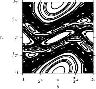
The phase space of the Chirikov’s map consists of regions of regular and chaotic motions. If the strength of the kick exceeds the specific value $k>0.97$, regular islands disappear, and the chaotic sea covers the whole phase space see Fig.(2) leading to a diffusive growth of the momentum in time (in the number of kicks) $\langle\big(p_{n}-p_{0}\big)^{2}\rangle=\frac{k^{2}}{2}n$. The kicked rotator is realized in a number of different physical setting. For example, in Ref.Komnik the model was employed to investigate spin systems. Contrary to the classical case, the quantum counterpart of the model Eq.(1)

shows a suppression of the diffusion due to the destructive role of quantum coherence Haake. Hence, instead of the diffusive growth localization occurs. We note, in both the classical and the quantum case the key issue is the discrete time evolution. The quantum kicked rotator can be mathematically mapped onto the one dimensional Anderson tight-binding model Anderson;

Here $W_{r}$ are the hopping amplitudes, the on-site energies $T_{m}$ are uniformly distributed in the interval $T_{m}\in[-T_{max}/2,T_{max}/2]$ and mimic the effect of randomly embedded impurities. Localization is indicated by the absence of mobility of electrons in the localized phase and the exponential decay of amplitudes of the wave functions. If the electron is initially localized around the site $n_{in}$, the probability to find the electron on the site $m$ exponentially decays $U_{m}^{(n_{in})}\approx\exp\big(-|n_{in}-m|/l_{c}\big)$ with the distance $|n_{in}-m|$, and the localization length is a function of energy $l_{c}\big(E\big)$. The Floquet operator $\hat{F}=\exp(-ik\hat{V}(\theta))\exp(-i\hat{p}^{2}/2)$ describes the evolution of the kicked rotator during the one period of driving. The unperturbed Hamiltonian $\hat{H}_{0}=\hat{p}^{2}/2$ is diagonal $\hat{p}|n\rangle=n|n\rangle$ in the eigenbasis $|n\rangle=\frac{1}{\sqrt{2\pi}}\exp(in\theta)$ of the momentum operator. Therefore, for the wave functions before and after the n-th kick we use the following ansatz

Here $|\psi^{+}(t+1)\rangle$ and $|\psi^{+}(t)\rangle$ are wave functions after the $n+1$-th and $n$-th kicks, while $|\psi^{-}(t)\rangle$ is the wave function before the $n$-th kick. For treating the free and kicked evolution parts, we utilize the following parametrization

leading to the following recurrent relations for the expansion coefficients:

Taking into account Eq.(I.1), Eq.(I.1) and Eq.(I.1) we deduce the quantum map for the expansion amplitudes in Eq.(I.1)

In the case $\hat{V}=\cos\theta$, the matrix element $J_{nm}=\langle m|\exp(-ikV(\theta))|n\rangle$ becomes Bessel functions. To find the equivalence between the kicked rotator and the Anderson model Eq.(4) we use the eigenfunctions and eigenvalues of the Floquet operator $\hat{F}|u^{+}\rangle=\exp(-i\phi)|u^{+}\rangle$, and consider the following identity $u^{-}(\theta)=\exp(ikV(\theta))u^{+}(\theta)$ in the $\theta$ representation. Taking into account $\exp(-i\phi)\hat{F}u^{+}(\theta)=\exp(-ikV)\exp(i(\phi-\hat{H}_{0}))u^{+}(\theta)=u^{+}(\theta)$ we obtain $u^{-}(\theta)=\exp(i(\phi-\hat{H}_{0}))u^{+}(\theta)$ or in the eigenbasis of $\hat{H}_{0}$ $u^{-}_{n}=\exp(i(\phi-n^{2}/2))u^{+}_{n}$. Let us introduce the auxiliary operator $\hat{W}$ defined as follows $\exp(-ik\hat{V})=\frac{1+i\hat{W}}{1-i\hat{W}}=\tan\big(\frac{k\hat{V}}{2}\big)$ and the vector $|u\rangle=\frac{1}{2}\big(|u^{+}\rangle+|u^{-}\rangle\big)$. Then, with the identity $u(\theta)=(1+i\hat{W})^{-1}u^{+}(\theta)=(1-i\hat{W})^{-1}u^{-}(\theta)$ we infer the operator equation:

or

Introducing the notations $T_{m}=i\frac{1-\exp(i(\phi-m^{2}/2))}{1+\exp(i(\phi-m^{2}/2))}=\tan\big((\phi-m^{2}/2)/2\big)$, $u_{m}\langle m|u\rangle$, $E=-W_{0}$, $W_{r}=\langle m|W|m+r\rangle$ we rewrite Eq.(10) in the matrix form

which demonstrates the mapping between the kicked rotator Eq.(3) and the Anderson tight-binding model Eq.(4). We note that the Anderson model, as well as the kicked rotator, describe single particle noninteracting systems. These models do not capture Many-body localization in interacting systems.

For nonlinear systems with a few degrees of freedom the coupling between different variables is decisive. At certain values of the coupling strength, the internal resonances overlap giving rise to Hamiltonian chaos and new phenomena such as Arnold’s diffusion in phase space Arnold. Let us introduce the canonical pair of action-angle variables:

and present theHamiltonian of the system in the form:

Here $H_{0}\big(I,\big),~~\forall~I_{i}\equiv I,i\in(1,..N)$ is the integrable part of the Hamiltonian and $V\big(I,\theta\big),~~\forall~\theta_{i}\equiv I,i\in(1,..N)$ is the perturbation. We presume that the Hamiltonian is not degenerate i.e. the Hessian $det|\frac{\partial\omega}{\partial I_{i}}|=det|\frac{\partial^{2}H_{0}}{\partial I_{i}\partial I_{j}}|\neq 0$ is not zero.
Following the Kolmogorov–Arnold–Moser (KAM) theorem one finds that the motion of an integrable system is confined to an invariant torus. If the system is subjected to a weak nonlinear perturbation, some of the invariant tori are deformed and survive.
The mechanism of Arnold’s diffusion is as follows: In the region of the destroyed invariant torus, in the vicinity of the internal resonances condition $\sum\limits_{j=1}^{N}n_{j}\omega_{j}=0,~~\forall~n_{j}\in\mathbb{N}$ a homocyclic structure emerges. The internal resonance condition determines a family of surfaces $H_{0}\big(I_{R}\big)=E$ with corresponding resonant action variables $I_{R}$. Nodal crossing points of different resonances construct a stochastic net. The Arnold’s diffusion sets in the stochastic net and is a topological generalization of classical kicked rotator problem. The Arnold’s diffusion was explored for the Heisenberg model, e.g., in Ref.Chotorlishvili1. The specific energy level statistics characterize the quantum counterpart of the classically chaotic nonlinear $D>2$ system Eq.(13). Depending on the symmetry of the Hamiltonian $\hat{H}$, in the region of destroyed phase space the invariant tori, according to the random matrix theory (RMT)Haake the mean inter-level energy distance $S=\langle E_{n+1}-E_{n}\rangle$ follows either a Gaussian orthogonal ensemble (GOE), a Gaussian unitary ensemble (GUE) or a Gaussian symplectic ensemble (GUE), respectively, i.e.

while for the integrable case the statistics is Poissonian $P(S)=\exp(-S)$. We note that the termination of the quantum Arnold’s diffusion for the particle moving in a quasi-1D waveguide was studied in Demikhovskii. The case $D=3/2$ was addressed in Ref. Chotorlishvili2. Classical chaotic Hamiltonian systems are insensitive to GOE, GUE, and GSE symmetries.

a The inverse participation ratio averages the fourth power of the wave function. It is positive for localized states and vanishes for extended states in the thermodynamic limit. If the wave function $|\psi_{i}\rangle$ at site $i$ of a tight-binding model is normalized then partition ratio $\hat{p}_{i}$ (PR) is given by

The inverse participation ratio (IPR) has been defined as

If the wave function spreads over $l$ lattice sites with equal amplitude $|\psi_{i}(r)|^{2}=1/l$ and vanishes elsewhere one can deduce $\hat{p}_{i}=l/N,~~\hat{P}_{i}=1/l$. As stated by F. WegnerWegner, PR describes the proportion of the total number of atoms in a system which contribute effectively to an eigenstate, whereas IPR is the inverse number of orbitals contributing effectively to this state. For localized states, IPR is larger than zero whereas PR vanishes in the thermodynamic limit. The wavefunction of the system shows anomalous scaling properties in the vicinity of the transition point to the localized phase. In particular, the ensemble averaged quantity Evers

shows fractal scaling properties with the characteristic size of the system $L$ and non-integer $\tau_{k}$. Here $\psi_{i}(r)$ is the amplitude of the eigenfunction $|i\rangle$ with the energy $e_{i}$ at site $r$ of the particle in a tight binding model and non-integer $\Delta_{k}\notin\mathbb{N}$.

Let us consider the simplest formulation of the scattering problem, a scattering of an electron on the $\delta$-like impurities located at $x=x_{0}$. The Schrödinger equation

admits the solution

and the continuity conditions

define the elements of the scattering matrix: $c_{out}=\begin{bmatrix}b^{+}\\ b^{-}\end{bmatrix}$ = $\begin{bmatrix}r&\acute{t}\\ t&\acute{r}\end{bmatrix}$ $\begin{bmatrix}a^{+}\\ a^{-}\end{bmatrix}$ = $S\begin{bmatrix}a^{+}\\ b^{-}\end{bmatrix}=Sc_{in}.$
Generally, the channel can be arbitrarily large and the dimension of the $t$ matrix is equal to the number of scattering channels. The explicit expressions of the $t$ matrix elements is obtained after solving Eq.(II.2) and expressing the coefficients $b^{+},b^{-}$ in terms of $a^{+},a^{-}$. The Landauer-Büttiker conductanceBeenakker is given by:

We note, a) When the system is in the localized phase, the eigenvalues of the transfer matrix are random numbers. However, there is a principle difference between RMT of quantum transport and chaotic nonlinear systems. The RMT describes quantum transport in terms of transmission eigenvalues of the open system (i.e., leads, impurities, etc.), while RMT is an internal property of nonlinear non-integrable quantum systems. The Thouless energy characterizes the energy scale of disordered conductors and is defined via the formula $E_{T}=\hbar D/L^{2}$, where $D$ is the diffusion constant, and $L$ is the characteristic size of the system. b) B. L. Altshuler and B. I. Shklovskii Altshuler; eeanderson showed that for energy separations greater than the Thouless energy $|E^{{}^{\prime}}-E|>E_{T}$, the correlation function deviates from random-matrix theory. If the condition $|E^{{}^{\prime}}-E|<E_{T}$ holds, the distribution function of eigenvalues of the transfer matrix read

Here $P\big(\{T_{n}\}\big)$ describes the correlated distribution of eigenvalues, $S=\langle E_{n+1}-E_{n}\rangle$ is the mean distance between neighboring eigenvalues, $\beta=1$ for GOE, $\beta=2$ for GUE, and $\beta=4$ for GSE symmetries, respectively, and the function $f(T_{k})$ is determined through the average spectral density $f(T_{k})=\int dT^{{}^{\prime}}_{k}\sigma(T^{{}^{\prime}}_{k})\ln|T_{k}-T^{{}^{\prime}}_{k}|$.