Magnus Hall Effect
Abstract
A new type of linear response Hall effect is predicted in time-reversal-invariant systems with built-in electric field at zero magnetic field. The Hall response results from a quantum Magnus effect where a self-rotating Bloch electron wavepacket moving under electric field develops an anomalous velocity in the transverse direction. We show that in the ballistic limit the Magnus Hall conductance measures the distribution of Berry curvature on the Fermi surface.
Introduction.— Studies of various Hall effects led to significant progress throughout the history of solid state physics. Starting with the classical Hall effectHall 1879, anomalous Hall effect Nagaosa et al. 2010, spin Hall effect Sinova et al. 2015, thermal Hall effect Banerjee et al. 2018; Kasahara et al. 2018, quantum Hall effect v. Klitzing et al. 1980, quantum spin Hall effect Kane and Mele 2005 and quantum anomalous Hall effect Haldane 1988; Chang et al. 2013; Liu et al. 2016 have been discovered. Among these, classical and anomalous Hall effects appear in time-reversal-breaking systems, where an applied electric field induces a transverse charge current.
An intrinsic contribution to anomalous Hall effect is associated with Berry curvature, a fundamental ingredient of modern band theory derived from electron’s wavefunction within the unit cell Karplus and Luttinger 1954. When a Bloch electron is accelerated under an electric field, the redistribution of electron density within the unit cell changes with increasing momentum, thus giving rise to an anomalous velocity proportional to Berry curvature. In time reversal breaking systems, total Berry curvature of occupied states can be nonzero, resulting in intrinsic anomalous Hall effect. The impact of Berry curvature on transport phenomena has attracted tremendous interest Xiao et al. 2010; Moore and Orenstein 2010; Morimoto et al. 2016; Morimoto and Nagaosa 2016; Chaudhary et al. 2018; Rudner and Song 2018.
On the other hand, there exists a large class of time-reversal-invariant, inversion-breaking materials which feature large Berry curvature in momentum space, especially near the gap edge or band crossing points. Examples include two-dimensional transition metal dichalcogenides (TMDs) Qian et al. 2014, graphene multilayers McCann and Koshino 2013; Rozhkov et al. 2016 and heterostructures Yankowitz et al. 2012, topological insulator surface states Fu 2009 and Weyl semimetals Hasan et al. 2017; Armitage et al. 2018; Yan and Felser 2017. Due to time reversal symmetry, the distribution of Berry curvature satisfies . It is an intriguing question whether such a distribution of Berry curvature with zero total can lead to any interesting phenomena in charge transport.
In this work, we demonstrate a new type of linear-response Hall effect induced by Berry curvature and built-in electric field in mesoscopic systems under time-reversal-symmetric condition. We consider electron transport in a Hall bar device made of a 2D material, such as bilayer graphene or transition metal dichalcogenide. In our setup, source and drain regions have different carrier densities, which can be achieved by local bottom gates. The difference in electrostatic potential energy due to bottom gates is accompanied by a built-in electric field in the junction at equilibrium, as shown in Fig. 1(a). We study electrical current in linear response to applied bias voltage . Since electrons moving from source to drain have nonzero net velocity, their wave packets can carry orbital angular momentum and nonzero net Berry curvature. The motion of chiral Bloch electrons under built-in electric field leads to a quantum analog of Magnus effect: as an electron traverses the junction, its center of wavepacket acquires a transverse shift. This in turn gives rise to a transverse current linearly proportional to the bias voltage, i.e., a Hall effect. We term this phenomenon “Magnus Hall effect”. It occurs in nonmagnetic systems at zero magnetic field, but relies on the built-in electric field. We show that in the ballistic limit, the Hall conductance is directly related to the Berry curvature distribution of the underlying material.
Magnus Hall effect is intimately related to nonlinear Hall effect, where recent theory predicted that in time-reversal-invariant materials the dipole moment of Berry curvature, i.e., Berry curvature dipole, can induce a nonlinear Hall effect, where the transverse current depends quadratically on the applied electric field Sodemann and Fu 2015. This phenomenon has been subsequently observed in bilayer WTe2 Ma et al. 2019; Kang et al. 2019. In the case of nonlinear Hall effect, reversing the electric field doesn’t change the transverse current. In Magnus Hall effect, transverse current is preserved under reversing both source-drain voltage and the direction of built-in electric field as presented in Fig.1(b). In an alternative scenario where the electric field arises from the source-drain voltage itself instead of bottom gates, the transverse current becomes second order in , resulting in nonlinear Hall effect. Our work thus opens a pathway to “Hall diodes” for high-frequency nonlinear transport based on quantum materials that have a significant distribution of Berry curvature.
Electronic Magnus effect.— First we shall consider an electron wave-packet which travels inside a sample. The sample has a short segment (between and ) within which there is spatially varying potential energy arising from different gate voltages on opposite sides (this corresponds to built-in electric field ). Inside this region, motion of the wave-packet is described by the semiclassical equations of motion Xiao et al. 2010:
| (1) |
Since the built-in electric field is small, wave packet momentum does not change substantially under acceleration. Therefore, the transit time through the electric field region of an incident electron with velocity is simply . During this time, the electron with will also travel in the direction. Importantly, between and there will be an additional displacement of wave packet along due to anomalous velocity. This displacement is given by:
| (2) |
with being the difference in potential energy. Therefore, an electron wave packet with non-zero Berry curvature moving through the region of electric field will acquire an additional shift in the direction perpendicular to the electric field as schematically shown in Fig. 1(a). This in turn leads to a current density in direction by integrating single wave-packet contribution over occupied states. This transverse current vanishes in equilibrium. However, in the current carrying state, the modes with positive and negative velocity are not equally occupied. Since in systems with time-reversal symmetry Berry curvature is opposite for and states (which also have opposite velocities), this effect can lead to a Hall current even in nonmagnetic materials. To see more clearly how the Hall current arises here, we employ Boltzmann transport equation.
Boltzmann transport equation solution.— To describe mesoscopic electron transport in a 2D system we use a collisionless Boltzmann equation (BE):
| (3) |
where is the occupation distribution function. Later we shall extend the discussion to non-ballistic case with finite relaxation time. We are looking for a stationary state distributions, so . We solve the Boltzmann equation in a geometry of a stripe of infinite width in direction and finite length in direction. At and we have a source and a drain. Since the system is translationally invariant in direction, the stationary distribution function will be independent of .
The wave packets evolve according to semiclassical equations given by Eq.(1). The energy of the electrons in the segment is:
| (4) |
where is the band energy. In equilibrium, the solution is given by Fermi-Dirac distribution with constant electrochemical potential , but with spatially changing energy (4) and can be expressed as:
| (5) |
is a solution of Boltzmann equation (3) as can be verified using Eqs.(1). This solution guarantees that no current is flowing in the system as at each energy and position the number of states with and is equal.
To obtain a solution that corresponds to a steady current flow, we apply a small bias in a form of imbalance of electrochemical potentials between source and drain, so that and . We have to solve BE with boundary conditions that take into account the presence of reservoirs at and . Taking into consideration the device geometry of our system, we now look for a solution in lowest order of the perturbation in the electrochemical potential imbalance. To achieve this, we write , where is the nonequilibrium part first order in the perturbation . This gives an equation for :
| (6) |
Since we assumed that is slowly varying, the second term on the left hand side is small, so we drop it and we arrive at . Therefore, only depends on . We can now determine its form from the boundary condition. The larger electrochemical potential of the source region results in a surplus of electrons entering the system at interface with positive velocity and propagating across the device without any scattering in the ballistic limit. This boundary condition gives us:
| (7) |
where . Equipped with this solution, we are able to calculate the longitudinal and Hall response of our system. We have then:
| (8) |
| (9) | ||||
| (10) |
Here term arises from Fermi surface anisotropy and depends on its orientation relative to the direction of applied bias . Note that is independent of . However, as we shall show later, this term can vanish due to symmetry.
To obtain the Hall current due to Berry curvature, we integrate the anomalous velocity contribution over the whole length of the device and then we can define Hall conductance as and obtain at :
| (11) |
where the electrostatic potential energy difference across the junction is assumed to be small.
This equation is the main result of this work. First of all, in the limit of small the Hall response does not depend on the detailed spatial dependence of the potential energy. Second, the dependence on is linear and the Hall current is independent of the system size in the ballistic limit. The effect is reduced by finite relaxation time as we show in Supplementary Materials. Crucially, Magnus Hall current is determined by directional Berry curvature of electrons with positive velocity along the direction of the applied bias. Therefore, by varying the bias with respect to crystal axis, Magnus Hall conductance can be used to map Berry curvature distribution on the Fermi surface.

Model.— To demonstrate this effect explicitly, we turn to a concrete model, which breaks inversion symmetry, but preserves time-reversal symmetry. We have chosen a simple two band model with the Hamiltonian:
| (12) |
It contains two massive Dirac cones which are tilted when . This model captures essential features of the tilted Dirac cones of topological crystalline insulator surface states Sodemann and Fu 2015 and low-energy band structure of 2D WTe2 Qian et al. 2014. More details of the model are presented in the Supplemental Materials.
We can now compute Berry curvature distribution in the Brillouin zone for parameters , which is shown in the inset of Fig.2 for the valence band. While the total Berry curvature integrated over Brillouin zone is equal to 0, the distribution consists of two peaks of opposite signs, located at the Dirac points.
Furthermore, this model possesses mirror symmetry , which guarantees that . For , this model has additional mirror symmetry . This symmetry is broken for . However, because the model is also time-reversal-invariant, we have , which causes the current density of Eq.(9) to vanish. Therefore, the Hall current will be determined solely by Magnus Hall contribution of Eq.(10) and can be calculated according to Eq. 11. Result of such a calculation is presented as the dashed curve in Fig.2 as a function of chemical potential. Even though the total integral of vanishes, because our result for only relies on the Berry curvature of Bloch states with , it is non-zero. For the set of parameters used in the calculation, both bands are symmetric with respect to line and so the result for the conduction band is mirror image of the curve for valence band. We note that the direction of the Hall current is the same for both bands, because while the Berry curvature switches sign to opposite between two bands, the velocities for given also change to opposite and as a results the integration occurs over regions with the same values of .
These approximate results derived from the semiclassical Boltzmann transport approach can be compared with a numerical tight-binding simulation using Landauer-Buttiker method. Details of the calculation are in Supplemental Materials. All the numerical simulations have been performed using Kwant package Groth et al. 2014. We consider the chemical potential dependence of , which we present as the solid curve in Fig. 2 for , lattice sites and . The curve is obtained by temperature broadening with . The qualitative behavior of the semiclassical result is reproduced with an asymmetric peak positioned away from the band bottom. The difference can be attributed to the differences in geometry of the setups for numerical simulation (finite width leads injecting current into the system) and semiclassical calculation (infinite width of the setup).

Candidate materials.— To observe the Magnus Hall effect under time-reversal symmetry, several conditions must be satisfied. First of all, the underlying material must break the inversion symmetry in order to have non-zero Berry curvature in the Brillouin zone. Furthermore, Berry curvature of right and left moving modes must be asymmetric. For example, under time-reversal symmetry massive Dirac fermions have to appear in pairs with opposite sign of Berry curvature. If they are isotropic, there will be an equal number of right movers with both signs of in each Dirac valley and their contributions will cancel each other. However, in general the Dirac cones are not perfectly isotropic and perfect cancellation will not occur. Two examples of materials that satisfy this condition are monolayer graphene on hBN (sublattice symmetry is broken due to formation of Moire superlatice) Park et al. 2008; Yankowitz et al. 2012; Hunt et al. 2013; Yankowitz et al. 2018 and bilayer graphene with perpendicular electric field applied McCann and Fal’ko 2006; McCann and Koshino 2013; Rozhkov et al. 2016. In both cases trigonal warping introduces asymmetry between right and left movers in each valley. Moreover, these platforms support devices of high quality, which enable ballistic motion of electrons Du et al. 2008; Mayorov et al. 2011; Banszerus et al. 2016, beneficial for observing the predicted effect.
As an example we use a model of bilayer graphene with trigonal warping and perpendicular electric field that opens up a gap. Calculations are performed using low-energy Hamiltonian that describes both and valleys of bilayer graphene (labeled by ) McCann and Fal’ko 2006:
| (13) |
where . Berry curvature distribution near both valleys is presented in the inset of Fig.3. The parameters used in the calculations are meV, m/s and with effective mass , being electron mass Mucha-Kruczyński et al. 2010; McCann and Koshino 2013. The Fermi surface at meV is indcated by the green line, solid for and dashed for . We can now use this to compute the Hall conductance as a function of chemical potential in the vicinity of the band edge, which is shown in Fig. 3 for meV. Our result demonstrates explicitly that Magnus Hall effect does not rely on Berry curvature dipole Sodemann and Fu 2015; Facio et al. 2018; Tsirkin et al. 2018; You et al. 2018; Zhang et al. 2018a; Zhang et al. 2018b; Shi and Song 2019 or the presence of skew scattering Isobe et al. 2018; Nandy and Sodemann 2019; König et al. 2018; Du et al. 2018 that are necessary conditions for nonlinear Hall effect.
Summary.— In this paper we have demonstrated existence of Magnus Hall effect in inversion symmetry breaking, but time reversal invariant systems that have non-zero Berry curvature. The effect relies on built-in electric field in the device and should be most pronounced in ballistic systems. The significance of the Magnus Hall effect is twofold. It opens a pathway to a new generation of current rectification devices. It also provides a much needed tool to map Berry curvature distribution of quantum materials in momentum space.
Acknowledgments.— We thank Hiroki Isobe and Su-Yang Xu for helpful discussions. This work was supported by DOE Office of Basic Energy Sciences, Division of Materials Sciences and Engineering under Award DE-SC0018945. MP was supported by Shell through the MIT Energy Initiative. LF was supported in part by a Simons Investigator Award from the Simons Foundation.
References
- Hall (1879) E. H. Hall, American Journal of Mathematics 2, 287 (1879).
- Nagaosa et al. (2010) N. Nagaosa, J. Sinova, S. Onoda, A. H. MacDonald, and N. P. Ong, Rev. Mod. Phys. 82, 1539 (2010).
- Sinova et al. (2015) J. Sinova, S. O. Valenzuela, J. Wunderlich, C. H. Back, and T. Jungwirth, Rev. Mod. Phys. 87, 1213 (2015).
- Banerjee et al. (2018) M. Banerjee, M. Heiblum, V. Umansky, D. E. Feldman, Y. Oreg, and A. Stern, Nature 559, 205 (2018).
- Kasahara et al. (2018) Y. Kasahara, T. Ohnishi, Y. Mizukami, O. Tanaka, S. Ma, K. Sugii, N. Kurita, H. Tanaka, J. Nasu, Y. Motome, T. Shibauchi, and Y. Matsuda, Nature 559, 227 (2018).
- v. Klitzing et al. (1980) K. v. Klitzing, G. Dorda, and M. Pepper, Phys. Rev. Lett. 45, 494 (1980).
- Kane and Mele (2005) C. L. Kane and E. J. Mele, Phys. Rev. Lett. 95, 226801 (2005).
- Haldane (1988) F. D. M. Haldane, Phys. Rev. Lett. 61, 2015 (1988).
- Chang et al. (2013) C.-Z. Chang, J. Zhang, X. Feng, J. Shen, Z. Zhang, M. Guo, K. Li, Y. Ou, P. Wei, L.-L. Wang, Z.-Q. Ji, Y. Feng, S. Ji, X. Chen, J. Jia, X. Dai, Z. Fang, S.-C. Zhang, K. He, Y. Wang, L. Lu, X.-C. Ma, and Q.-K. Xue, Science 340, 167 (2013).
- Liu et al. (2016) C.-X. Liu, S.-C. Zhang, and X.-L. Qi, Annu. Rev. Condens. Matter Phys. 7, 301 (2016).
- Karplus and Luttinger (1954) R. Karplus and J. M. Luttinger, Phys. Rev. 95, 1154 (1954).
- Xiao et al. (2010) D. Xiao, M.-C. Chang, and Q. Niu, Rev. Mod. Phys. 82, 1959 (2010).
- Moore and Orenstein (2010) J. E. Moore and J. Orenstein, Phys. Rev. Lett. 105, 026805 (2010).
- Morimoto et al. (2016) T. Morimoto, S. Zhong, J. Orenstein, and J. E. Moore, Phys. Rev. B 94, 245121 (2016).
- Morimoto and Nagaosa (2016) T. Morimoto and N. Nagaosa, Science Advances 2, e1501524 (2016).
- Chaudhary et al. (2018) S. Chaudhary, M. Endres, and G. Refael, Phys. Rev. B 98, 064310 (2018).
- Rudner and Song (2018) M. S. Rudner and J. C. W. Song, arXiv:1807.01708 (2018).
- Qian et al. (2014) X. Qian, J. Liu, L. Fu, and J. Li, Science 346, 1344 (2014).
- McCann and Koshino (2013) E. McCann and M. Koshino, Rep. Prog. Phys. 76, 056503 (2013).
- Rozhkov et al. (2016) A. V. Rozhkov, A. O. Sboychakov, A. L. Rakhmanov, and F. Nori, Physics Reports 648, 1 (2016).
- Yankowitz et al. (2012) M. Yankowitz, J. Xue, D. Cormode, J. D. Sanchez-Yamagishi, K. Watanabe, T. Taniguchi, P. Jarillo-Herrero, P. Jacquod, and B. J. LeRoy, Nature Physics 8, 382 (2012).
- Fu (2009) L. Fu, Phys. Rev. Lett. 103, 266801 (2009).
- Hasan et al. (2017) M. Z. Hasan, S.-Y. Xu, I. Belopolski, and S.-M. Huang, Annu. Rev. Condens. Matter Phys. 8, 289 (2017).
- Armitage et al. (2018) N. P. Armitage, E. J. Mele, and A. Vishwanath, Rev. Mod. Phys. 90, 015001 (2018).
- Yan and Felser (2017) B. Yan and C. Felser, Annu. Rev. Condens. Matter Phys. 8, 337 (2017).
- Sodemann and Fu (2015) I. Sodemann and L. Fu, Phys. Rev. Lett. 115, 216806 (2015).
- Ma et al. (2019) Q. Ma, S.-Y. Xu, H. Shen, D. MacNeill, V. Fatemi, T.-R. Chang, A. M. M. Valdivia, S. Wu, Z. Du, C.-H. Hsu, S. Fang, Q. D. Gibson, K. Watanabe, T. Taniguchi, R. J. Cava, E. Kaxiras, H.-Z. Lu, H. Lin, L. Fu, N. Gedik, and P. Jarillo-Herrero, Nature 565, 337 (2019).
- Kang et al. (2019) K. Kang, T. Li, E. Sohn, J. Shan, and K. F. Mak, Nature Materials 18, 324 (2019).
- Groth et al. (2014) C. W. Groth, M. Wimmer, A. R. Akhmerov, and X. Waintal, New J. Phys. 16, 063065 (2014).
- Park et al. (2008) C.-H. Park, L. Yang, Y.-W. Son, M. L. Cohen, and S. G. Louie, Phys. Rev. Lett. 101, 126804 (2008).
- Hunt et al. (2013) B. Hunt, J. D. Sanchez-Yamagishi, A. F. Young, M. Yankowitz, B. J. LeRoy, K. Watanabe, T. Taniguchi, P. Moon, M. Koshino, P. Jarillo-Herrero, and R. C. Ashoori, Science 340, 1427 (2013).
- Yankowitz et al. (2018) M. Yankowitz, J. Jung, E. Laksono, N. Leconte, B. L. Chittari, K. Watanabe, T. Taniguchi, S. Adam, D. Graf, and C. R. Dean, Nature 557, 404 (2018).
- McCann and Fal’ko (2006) E. McCann and V. I. Fal’ko, Phys. Rev. Lett. 96, 086805 (2006).
- Du et al. (2008) X. Du, I. Skachko, A. Barker, and E. Y. Andrei, Nature Nanotechnology 3, 491 (2008).
- Mayorov et al. (2011) A. S. Mayorov, R. V. Gorbachev, S. V. Morozov, L. Britnell, R. Jalil, L. A. Ponomarenko, P. Blake, K. S. Novoselov, K. Watanabe, T. Taniguchi, and A. K. Geim, Nano Lett. 11, 2396 (2011).
- Banszerus et al. (2016) L. Banszerus, M. Schmitz, S. Engels, M. Goldsche, K. Watanabe, T. Taniguchi, B. Beschoten, and C. Stampfer, Nano Lett. 16, 1387 (2016).
- Mucha-Kruczyński et al. (2010) M. Mucha-Kruczyński, E. McCann, and V. I. Fal’ko, Semicond. Sci. Technol. 25, 033001 (2010).
- Facio et al. (2018) J. I. Facio, D. Efremov, K. Koepernik, J.-S. You, I. Sodemann, and J. van den Brink, Phys. Rev. Lett. 121, 246403 (2018).
- Tsirkin et al. (2018) S. S. Tsirkin, P. A. Puente, and I. Souza, Phys. Rev. B 97, 035158 (2018).
- You et al. (2018) J.-S. You, S. Fang, S.-Y. Xu, E. Kaxiras, and T. Low, Phys. Rev. B 98, 121109 (2018).
- Zhang et al. (2018a) Y. Zhang, Y. Sun, and B. Yan, Phys. Rev. B 97, 041101 (2018a).
- Zhang et al. (2018b) Y. Zhang, J. van den Brink, C. Felser, and B. Yan, 2D Mater. 5, 044001 (2018b).
- Shi and Song (2019) L.-k. Shi and J. C. W. Song, Phys. Rev. B 99, 035403 (2019).
- Isobe et al. (2018) H. Isobe, S.-Y. Xu, and L. Fu, arXiv:1812.08162 (2018).
- Nandy and Sodemann (2019) S. Nandy and I. Sodemann, arXiv:1901.04467 (2019).
- König et al. (2018) E. J. König, M. Dzero, A. Levchenko, and D. A. Pesin, arXiv:1812.06989 (2018).
- Du et al. (2018) Z. Z. Du, C. M. Wang, S. Li, H.-Z. Lu, and X. C. Xie, arXiv:1812.08377 (2018).
Supplemental Material for
”Magnus Hall effect”
Finite relaxation time.— To take into account the effects of scattering, we use Boltzmann equation (BE) in relaxation time approximation:
| (S1) |
where is the occupation distribution function, is the equilibrium distribution and is the relaxation time. We solve the Boltzmann equation in the same geometry as in the main text, but allow for a rotation of the direction of applied bias (parallel to the direction of built-in electric field) with respect to Fermi surface orientation. We label the direction parallel to the bias direction as , where is an arbitrary angle that represents rotation of the device with respect to underlying crystal, which we keep fixed. This allows to account for dependence of the Hall current on anisotropy of the Fermi surface. The gate-induced electrostatic potential is now labeled (with being the coordinate along , so that ). Taking into consideration the device geometry of our system, the Boltzmann equation assumes the form:
| (S2) |
We again look for a solution in the lowest order of perturbation in , so we write , where is the nonequilibrium part first order in the perturbation. This gives an equation for :
| (S3) |
Due to weak variation of , we can drop second term on the right hand side and using we arrive at:
| (S4) |
The general solution of this equation is:
| (S5) |
We can now determine and from the boundary condition similarly to the main text. Since the source has a larger electrochemical potential, it results in a surplus of electrons entering the system at with positive velocity. If the system is ballistic (), these electrons propagate across the device without any scattering. When disorder is introduced into the sample, finite relaxation time will result in exponential decay of the surplus distribution. Therefore we have:
| (S6) |
Therefore, in the simplest generalization to the case with finite relaxation time the distribution of surplus electrons that exit the source region will decay exponentially on the length scale comparable to mean free path . Thus, the effect of disorder on Magnus Hall effect will be suppressed as long as the device length is shorter than mean free path.
Additional details of the two band model.—As an example of a model which exhibits Magnus Hall effect we proposed a model with the Hamiltonian:
| (S7) |
which preserves time-reversal, but breaks inversion symmetry for . It consists of 2 bands of different effective masses determined by and which hybridize with a -dependent term. Parameter controls the band gap at point and if the bands are inverted around that point. When the spectrum of this Hamiltonian is degenerate at two points in the Brillouin zone and the dispersion can be linearized in their vicinity, giving two Dirac cones. These cones are tilted when . To get non-zero Berry curvature, one has to break inversion symmetry to observe the effects described in the main text section. Since we are interested in the Hall effect while time-reversal symmetry is preserved and the integral of Berry curvature over Brillouin zone vanishes, we have to break inversion symmetry with . This adds mass to both of the Dirac cones, opening a band gap. This is presented in Fig.S1, which shows the band structure along and directions for parameters . This choice of parameters corresponds to rotationally symmetric spectrum close to the Dirac points.
Details of numerical simulations and additional results.— To perform Landauer-Buttiker simulation, we discretize the continuum Hamiltonian (12) on a square lattice with lattice constant . The potential energy drop is included as a spatially varying onsite energy given by:
| (S8) |
In the simulations we used and . The scattering region is a rectangle that consists of lattice sites and to each of the sides of the device we attach a semi-infinite lead of width that is equal to the length of that particular side (as shown in inset of Fig. S2). The leads are described by the same Hamiltonian as the scattering region and they also include potential to ensure no mismatch at the lead-scattering region interface. In such a setup we compute the scattering matrices for varying chemical potential , system sizes and potential energy change . From scattering matrices we obtain transmission probabilities for each pair of leads and then calculate . We use it to calculate voltages at each of the leads in two cases: (1) current flowing between leads 1 and 2 (leads 3 and 4 serve as voltage probes only) and (2) current flowing between leads 3 and 4 (leads 1 and 2 serve as voltage probes only). For each case we then define and . We can now setup a set of linear equations:
| (S9) | |||
From this we can then obtain , , and for the sample. The value will correspond to as used for comparison with semiclassical calculation in the main text.
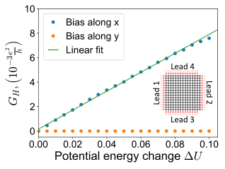
In Fig. S2 we show dependence of Hall conductance on the potential energy change for and system size , . When chemical potential imbalance is applied along direction, Hall conductance increases linearly with before eventually acquiring some nonlinear contribution. This is shown by a least-squares linear fit to the simulation results and is consistent with the semiclassical calculation. Finally, when we rotate our setup by 90∘, effectively applying bias and potential difference along direction of the model, the result is zero independent of potential energy change, which in semiclassical formalism corresponds to vanishing of the Berry curvature integral due to symmetry.
In Fig.S3 we present longitudinal conductance obtained using the numerical simulation as a solution of Eq.(S9) (solid line) and from semiclassical calculation presented in the main text (dashed line). The deviation is mainly due to omission of the built-in electric field effect in the semiclassical calculaton.